RIGIDITY PERCOLATION IN DISORDERED FIBER SYSTEMS: THEORY AND APPLICATIONS
Samuel Blackwell Heroy
A dissertation submitted to the faculty of the University of North Carolina at Chapel Hill in partial fulfillment of the requirements for the degree of Doctor of Philosophy in the
Department of Mathematics.
Chapel Hill 2018
Approved by:
Peter J. Mucha
M. Gregory Forest
Daphne Klotsa
David Adalsteinnson
©2018
ABSTRACT
Samuel Blackwell Heroy: Rigidity Percolation in Disordered Fiber Systems: Theory and Applications
(Under the direction of Peter J. Mucha)
Nanocomposites, particularly carbon nanocomposites, find many applications spanning an impressive variety of industries on account of their impressive properties and versatility. However, the discrepancy between the performance of individual nanoparticles and that of nanocomposites suggests continued technological development and better theoretical understanding will provide much opportunity for further property enhancement. Study of computational renderings of disordered fiber systems has been successful in various nanocomposite modeling applications, particularly toward the characterization of electrical properties. Motivated by these successes, I develop an explanatory model for ‘mechanical’ or ‘rheological percolation,’ terms used by experimentalists to describe a nonlinear increase in elastic modulus/strength that occurs at particle inclusion volume fractions well above the electrical percolation threshold. Specifically, I formalize a hypothesis given by Penu et al. (2012), which states that these dramatic gains result from the formation of a ‘rigid CNT network.’ Idealizing particle interactions as hinges, this amounts to the network property of rigidity percolation—the emergence of a giant component (within the inclusion contact network) that is not only connected, but furthermore the inherent contacts are patterned to constrain all internal degrees of freedom in the component.
ACKNOWLEDGEMENTS
From my advisors, Drs. Peter J. Mucha and M. Gregory Forest, I simply could not ask anything more. How does one get two top tier advisors to guide his or her doctoral study? I have no idea, but it happened to me, and it will shape not only this research, but my entire career. In addition to their formal involvement in my PhD committee, the rest of my committee has also been indispensable to my research and each member has been a joy to work with. Dr. Daphne Klotsa’s course on soft matter research helped me to understand how geometry underplays a large body of the materials research canon, besides being one of the most enjoyable classes I have had in graduate school. Both she and Dr. Theo Dingemans, professors in the Applied Physical Sciences department at UNC, have provided great and advice helped me guide my research towards realistic applications as part of a mathematics/applied physical sciences collaborative group. While Dr. David Adalsteinsson has been less directly involved with my research, he has proved very helpful whenever I have met with him, and his introductory course on scientific computation has helped guide my overall understanding of this field.
Several people have contributed greatly to the development of my research and scholarly activity over the years—first and foremost, Drs. Dane Taylor (SUNY-Buffalo) and Feng “Bill” Shi, have been highly involved in my research as postdoctoral research associates and as young faculty members. In particular, the idea of rigid graph compression was originally conceived by Dr. Taylor, while much of the code I use has roots in Dr. Shi’s work. Dr. Maruti Hegde, a staff scientist working for Dr. Dingemans, has provided great scientific understanding, while Ryan Fox and Minzhi Jiang, graduate students in the Applied Physical Sciences department, have done the same within our mathematics/applied physical sciences collaborative group. Laurie Straube, Sara Kross, and Jean Foushee-Tyson (staff in UNC mathematics office) have been incredibly helpful in constantly looking out for me as well as all the students within our department over these five years.
academically or simply morally—especially, in alphabetical order—Manuchehr Aminian, Aaron Barrett, Dr. Nicholas Battista, Francesca Bernardi, Emma Buckingham, Brandon Byers, Alyssa Byrnes, Martin Dewitt, Colin Guider, Dr. Alex Hoover, Dr. Caitlin Hult, Zeliha Kihilic¸, Dr. Michael Malahe, Laura Manuel, Katri Morgan, Dr. John Palowitch, Jacob Perry, Dr. Ian Phillipe, Andrew Prudhom, David Raps, Dr. Quentin Robinson, Sean Rogers, Dr. Saray Shai, Alexis Sparko, Dr. Natalie Stanley, Aditi and Shirish Sundareson, Sterling Swygert, Charlie Talbot, Ben Vadala Roth, William Weir, Caroline Yang,... Finally, of course none of this would be possible without the full support of my family–Anna, Bill, Rob, Katie, Alex, Jessica, Katie, and Gigi.
PREFACE
TABLE OF CONTENTS
LIST OF FIGURES . . . xi
LIST OF ABBREVIATIONS AND SYMBOLS . . . .xviii
1 CHAPTER 1: INTRODUCTION . . . 1
1.1 Overview . . . 1
1.2 Modeling of nanocomposites’ electrical properties . . . 2
1.3 Mechanical percolation . . . 4
1.3.1 Experimental characterizations . . . 4
1.3.2 Rigidity: a microstructural mechanism for mechanical percolation? . . . 5
1.4 Outline of the dissertation . . . 7
2 CHAPTER 2: RIGID GRAPH COMPRESSION . . . 9
2.1 Overview . . . 9
2.2 Previous methods . . . 10
2.2.1 Maxwell counting . . . 10
2.2.2 Laman, the pebble game, and Henneberg constructions . . . 11
2.2.3 Rigidity matroid theory . . . 12
2.2.4 Relationship to rigidity percolation in disordered Particle systems . . . 13
2.3 Motif-based rigidity decomposition . . . 14
2.3.1 Rigidity matroid theory for interacting rigid components . . . 15
2.3.2 Algorithmic framework for Rigid Graph Compression . . . 16
3 CHAPTER 3: RIGIDITY PERCOLATION IN DISORDERED SYSTEMS OF TWO-DIMENSIONAL FIBERS . . . 18
3.2 Primitive rigid motifs in two dimensions . . . 18
3.3 Algorithmic details of Rigid Graph Compression applied to 2D disordered fiber systems (2D-RGC-5) . . . 27
3.4 Numerical experiments . . . 30
3.4.1 Experimental design . . . 30
3.4.2 Results . . . 31
3.5 Related directions . . . 34
4 CHAPTER 4: RIGIDITY PERCOLATION IN DISORDERED SYSTEMS OF THREE-DIMENSIONAL FIBERS . . . 36
4.1 Overview . . . 36
4.2 Primitive 3D rigid motifs . . . 36
4.2.1 Differences between rigidity analysis in 2 and 3 dimensions . . . 36
4.2.2 Primitive rigid motifs in three dimensions . . . 38
4.3 Algorithmic implementation . . . 47
4.4 Numerical experiments . . . 50
4.4.1 Experimental design . . . 50
4.4.2 Results . . . 53
4.4.3 A note about computational efficiency . . . 54
4.5 Accuracy of the rigidity percolation threshold estimation . . . 56
4.6 Maxwell prediction . . . 58
5 CHAPTER 5: CHARACTERIZATION OF NANOCOMPOSITES WITH IN-TERFACIAL CRYSTALLINE GROWTH . . . 60
5.1 Overview . . . 60
5.1.1 Description of experimental system . . . 60
5.1.2 Modeling goals . . . 61
5.2 Geometric characterization of CNT-facilitated crystallinity . . . 62
5.2.1 Probabilistic modeling . . . 62
5.3.1 Models for heterogeneous CNT dispersions . . . 69
5.4 Network-based assessments for property characterization . . . 71
5.4.1 Numerical experiments . . . 73
6 CHAPTER 6: CONCLUSIONS AND FUTURE DIRECTIONS . . . 77
LIST OF FIGURES
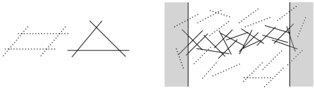
1.1 Rigidity in two-dimensional rod-hinge systems. Left: Supposing that rods interact as hinges at intersections, four rods connected pairwise in two dimensions are ‘floppy’ (dotted) in that they may deform through different interior angles, whereas three rods connected pairwise are ‘rigid’ (solid). Right: A large component of mutually rigid rods may add mechanical stability to a host composite. I use rigidity characterization algorithms to detect the presence of such a component connecting two boundaries (vertical rods) bounding a large computational domain. In order to keep the rod distribution uniform throughout the (white) domain, I allow rods to be placed in the ‘buffer’ regions (grey rectangles) on the exterior sides
of the boundaries. . . 6
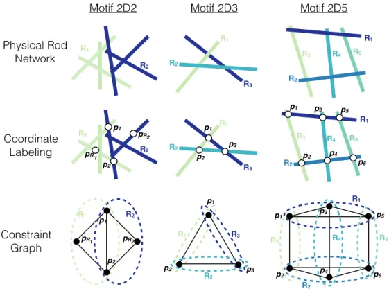
3.1 Derivation of three primitive rigid motifs for 2D rod-hinge systems. Top Row: Rigid components, which may be individual rods or sets of connected rods, distinguished here by color, intersect with three specific topologies as described in Sec. 3.2 to form larger-scale rigid components: (left column) two rigid componentsR1 andR2 interacting at a pair of
points; (middle column) three rigid componentsR1,R2andR3interacting
pairwise; and (right column) five rigid components,R1, . . . , R5interacting
in an identified pattern. For simplicity, I depict the rigid bodies in the middle and right columns as rods, but the proofs are general to include composite rigid components.Middle Row: Coordinate labelings are affixed to each rigid component: three noncollinear points are required to describe the motions of a 2D rigid component consisting of multiple rods, whereas individual rods are 1D and require only two points (although more may be used).For each motif, I identify a set of minimal coordinate labelings that include intersection points whenever possible (see text for clarification). Bottom Row: The coordinate labelings give rise to constraint graphs in which edges (black lines) indicate distances between adjacent points that are fixed. The dashed ellipses group the rigid components to which these points belong. By Theorems 3.1, 3.2, and 3.3, these constraint graphs and
the motifs that generated them are rigid in two dimensions. . . 19
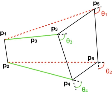
3.2 Visualization of quantities of interest in Eqs. 3.11.Given thatp1,p3,p5
andp2,p4,p6form noncollinear sets, the variables|∆p1,5|,|∆p2,6|,θ1,
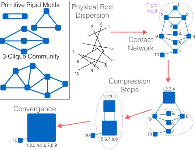
3.3 Graph compression of rod-hinge systems using rigid motifsUsing a 10-component rod-hinge system as an example, I describe 2D-RGC-5 (Algorithm 2), which iteratively compresses 2- and 5-component primitive rigid motifs, as well as 3-clique communities (see top left inset for contact network representations of these motifs). In the first step, the physical rod dispersion is transformed into a rod contact network. This contact network contains both a 3-clique community (nodes 1-4) and a 5-component motif (5-9). In two steps, each of these motifs are compressed into a single compound node. These two composite nodes are connect by two edges, which is the 2-component primitive rigid motif and is then compressed in the final step, giving one compound node representing rods 1-9 connected to another node representing rod 10. Stopping in the absence of any other primitive rigid motifs, RGC thus identifies two rigid components within
the candidate rod-hinge system. . . 28
3.4 Nonisomorphic intersections of 2-, 3-, and 5-component motifs. Top Row: Simplest nonisomorphic cases involving intersections of (that is, containing both) the 2- and 3-body primitive rigid motifs. Middle Row: Simplest intersections of 2- and 5-component motifs. Bottom Row: Sim-plest intersections of 3- and 5-component motifs. Each of these networks compress to a single rigid component regardless of the order in which the
2D primitive rigid motifs are compressed. . . 30
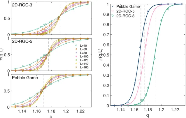
3.5 Comparison of 2D-RGC-3, 2D-RGC-5, and pebble-game algorithms for 2D rigidity percolation. Left: For all three rigidity-detection algo-rithms, there is a phase transition inπ(q, L)that becomes sharper with increasingL—an extrapolation algorithm is used to estimate rigidity perco-lation thresholds (vertical dashed lines) from these individual curves. The transitions identified using the RGC algorithms approximate that of the pebble game, with that of the2D-RGC-5being the closer approximation. Incorporation of yet more rigid motifs would further increase the accuracy of this approximation.Right: Rigidity percolation transitions for each of
the three algorithms are displayed for a large domain size,L= 140. . . 31
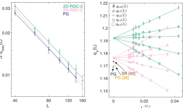
3.6 Estimation of correlation length exponent and rigidity percolation threshold for RGC and pebble game algorithms. Left: Using each rigidity characterization algorithm, I use the relation∆qmin(L)∼L−1/ν
to estimateν. Right: An extrapolation scheme is used to estimateqmin
using each of the three rigidity detection algorithms. For comparison, I display the rigidity percolation threshold found in (Latva-Kokko and M¨akinen, 2001) using the pebble game (PG [26]), in my own pebble game calculations (PG), and in (Wilhelm and Frey, 2003) using spring relaxation
(SR). . . 32
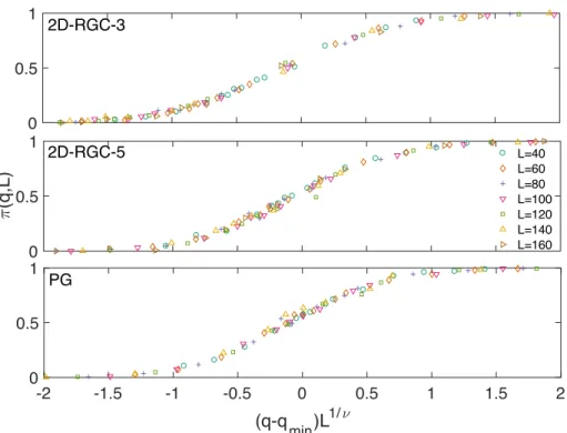
3.7 Demonstration of data collapse. Using the identified values ofν and qminfor each rigidity detection algorithm, I find the data collapse
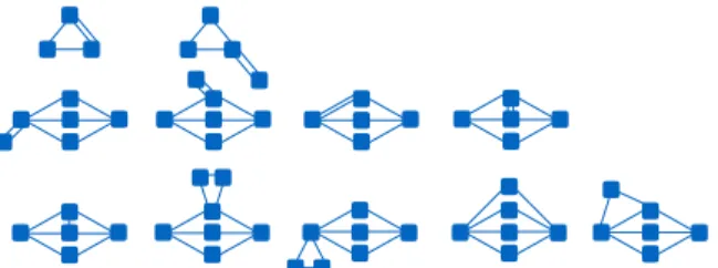
3.8 Rigid motifs not identified by 2D-RGC-3 and/or 2D-RGC-5. Exhaus-tive search of rod contact networks containing up to seven rods reveals seven rigid motifs incorrectly identified as floppy by 2D-RGC-3 only (yellow), and three other rigid motifs incorrectly identified as floppy by both 2D-RGC-3 and 2D-RGC-5 (purple). These latter motifs—which are classified as rigid via the pebble game—could potentially be incorporated
into a 2D-RGC-7 algorithm. . . 35
4.1 If{p2,p3,p4,p5} is noncollinear, then{p2,p3,p4}and {p2,p3,p5}
cannot simultaneously be collinear.. . . 42 4.2 Seven motifs featuring individual rods (small) and other non-axisymmetric
(nr >1) rigid components (big) are proven to be rigid in Sec. 4.2. In the rod contact graph representation, nodes represent rigid components and edges represent contacts. These images do not depict certain conditions
regarding which constacts may or may not be rod-sharing. . . 47
4.3 Different orderings of motif compression in3D-RGCcan give differ-ent results for certain graphs. Left: The top five-node graph could be compressed into either four nodes (viaMotif 3D2B) or two nodes (3D4a). Depending on whether the objective is to reduce the number of vertices in the graph, or to agglomerate the most rods into a single node (greedily), one or the other option may be preferable. Right: Even in the initial identi-fication/compression of3-clique communities, choices must be made—the base contact graph can be compressed into either four or three nodes, depending on which 3-clique community is compressed first. Graphs with adjacent3-clique communitiescould be compressed in alternative ways, as shown here. In the implementation of the next section,3-clique com-munitieswill be compressed greedily (the largest will be compressed first, as in the right path which leaves three nodes). Note that such a choice is not necessary in two dimensions, wherein2D-RGC-5need not distinguish whether a node represents a rod or a larger rigid body (giving that any adjacent 3-clique communities are mutually rigid). An observation related to this problem is that the middle node—that shared by both 3-clique communities—is rigid with respect to either 3-clique community, but the algorithm of3D-RGCnecessitates that it be identified as being part of a
4.4 Differing definitions of rigidity percolation. Top: Two rod dispersions contain rigid components that are identified as spanning by either defi-nition (I) or (II) but not both. In the left configuration, the boundaries template growth of the rigid component, which is spanning according to definition (I). Only the triangle of touching rods is identified as rigid if the boundary nodes are not present, and because this triangle intersects only the right boundary, it is not spanning according to (II). In the right, the entire component is rigid without the boundary nodes. Because the com-ponent intersects both boundaries, it is rigid according to definition (II). However, if boundary nodes were introduced, this component would be singly connected to each boundary node and thus would not be identified as spanning by (I). The case of the left panel (II but not I) occurs with far greater frequency in simulation (see Fig. 4.6).Bottom: If boundary nodes are introduced as in definition (I), 3D-RGC identifies two components in the initial 3-clique community compression—these are the magenta rods in one component, and both the red and black rods together in one component. The latter component is a 3-clique community only if the boundary node is included—it fragments into the red triangle of rods (one 3-clique community) and assorted rods if the corresponding boundary node is not included. Consequentially, this configuration (including∼90 rods excluded from this depiction for clarity) is identified as having a spanning rigid component according to definition (I) but not (II) after full
implementation of3D-RGC.. . . 52
4.5 Rigidity Percolation as Measured by Three Definitions. While the rigidity percolation threshold corresponding to definition I is be lower than that corresponding to II for any finiteL, these thresholds seem to converge asL→ ∞(see Fig. 4.6). The dependence of the relative size of
the largest rigid component onLandφseems to be similar to that ofπII. . . 54
4.6 Finite-size scaling analysis (top) and data collapse (bottom) for rigid-ity percolation as measured by (I) and (II).Using the standard scaling analysis of Stauffer and Aharony (1992), I find thatπI(L) = ΠI([φ−
0.0604]L1/0.728)and thatπII(L) = ΠII([φ−0.0603]L1/0.978). . . 55
4.7 Scaling of 3D-RGC as currently implemented. Computational effi-ciency could surely improved, but the current implementation is sufficient
4.8 Graphlet-based analysis of the accuracy of3D-RGCLeft: The sufficient but necessary algorithm 3D-RGC identifies as rigid all those graphlets containing at most5vertices (i.e.nr≤5), which both satisfy the Maxwell counting condition (Eq. 4.14) and the requirement that a rigid graph is contained in its2-core. These latter two conditions are necessary but not sufficient for rigidity—9graphlets of size|V| = 6(signifyingnr = 6) and57of size|V|= 7meet these latter conditions but are not classified as rigid by3D-RGC. Of these57, only24do not contain one of the former |V| = 6 candidate motifs as a subgraph, and thus merit consideration. Right: Upon further inspection, two of the|V| = 6 graphlets are rigid when viewed as rod contact networks—the other seven satisfy 4.14 and
are contained in their2-cores but are nonetheless floppy. . . 58
4.9 Comparison of Maxwell prediction with observed rigidity percolation threshold.Left: The rod contact equation seems to slightly overpredict the mean number of contacts per rod in these simulations (only one box size is used in this graphic, but symbols overlap completely when the six sizes are included). This overprediction may be either the result of some slight approximations used in the employment of periodic boundary conditions, or of correlations between contacts not considered in the equation’s deriva-tion.Right: Curiously, the Maxwell prediction2Nc/nr = 10/3seems to be quite accurate only when the degree zero nodes are not included in this calculation. Information from all six box sizes is used in this box (with
colors corresponding to those of Fig. 4.5). . . 59
5.1 Favorable interactions between the polyimide and CNTs give rise to a third phase of crystal coating.The principal ingredients of the nanocom-posite of interest are the amorphous polyetherimide 3,3’,4,4’-oxdiphthalic dianhydride (ODPA-P3), shown left—and single walled carbon nanotubes
(SWCNTs), shown right. . . 61
5.2 Observed CNT agglomeration guides simulation-based study. Left: On account of Van der Waals attractions, chemical bonds, and impurities, CNTs tend to agglomerate—while sonication and other procedures are frequently used to disaggregate them, it is highly difficult to attain a dis-persion that can be considered anything close to uniform. The film shown in this optical microscopy image corresponds to the study introduced in Sec. 5.1.1 and discussed throughout this chapter. Here, PEI is shown to crystallize around CNTs of concentration φc = 0.001(Figure adapted from Hegde et al. 2013). Right: In order to mimic the CNT/crystal distri-bution observed in microscopy, a simple spatial model (theMat´ernprocess
5.3 Statistical fitting results for various models of crystalline growth about CNTs. Left: Three simple models (indicated by line style) are used to predict total crystallinity for four different CNT loadings (indicated by color) as a function of maximum radial crystalline growthγmax. For each value ofφcandγmax, there is an obvious ordering ofVcryspredictions (the unimpeded growth model predicts the greatest crystallinity followed by the homogenous geometric model and then by the heterogeneous crystalline model). Experimental measurements of crystallinity (Hegde et al., 2013) as a function ofφcare fit using each model to inverse predictγmax—the predictions of the three models areγc+γmax= 3.0,. 3.5,4.0nm for each of the respective models, as indicated by vertical lines.Right: The simple models are here used to predict Young’s modulus as a function of radial crystalline growth for the four different CNT loadings considered exper-imentally. No fitting of the displayed experimental data is undertaken. Rather, the vertical lines correspond to the inverse predictions of γmax
given in the left figure. . . 67
5.4 Basic approach of discrete geometric characterization schemeLeft: In this 2D schematic of the discretized geometric characterization approach, CNTs (fuzzy) are first discretized into n` evenly spaced points apiece along their central axes (the local endpoints must also be selected). Then, a KD-tree is used to determine which voxels (squares) have centroids within some radiusγc+γmaxof the rod point cloud (teal circles represent the coverage of this point cloud). Voxels identified as occupied are here marked as red-bordered squares, while the others have black border. Note that some voxels that are counted vacant may have some volume within the crystal/CNT-occupied regions, while some counted occupied have some volume not within such regions–the fineness of the approximation is controlled by`nandLv.Right: In this 3D realization, voxels identified as
occupied are denoted by red points, which surround their nucleating CNTs. . . 68
5.5 Accuracy of discrete geometric characterizationLeft: Estimations of crystallinity converge asLv →0—treating the calculation withLv = 0.5 nm as ground truth, I calculate the percent error for varying γmax in characterization routines wherein the chosen voxel size varies between50 and1nm. For the rest of the simulations in this study, I balance accuracy and efficiency in choosingLv = 2nm.Right: When implemented on CNT dispersions of uniform position and orientation (with periodic boundary conditions), the discretized geometric approach agrees strongly with the homogeneous geometric model. Error bars are not shown here but standard
deviations (across the five different samples per point) are smaller than plot symbols. 69
5.6 Discrete geometric characterization of heterogeneous CNT dispersions Left: Atφc= 0.001(left) andφc= 0.003(right), the dispersion param-eters λs and γM (if the process is Mat´ern) or σ (Thomas) affects the calculation of crystallinity, as more clustered dispersions are marked by crowding and less efficient growth. For each curve, data points represent
5.7 Experimental characterization of nanocomposite strength. Whereas experimental data shows clearly that increasing CNT vol % (or volume fraction) gives a higher modulus, the relationship between % CNTs and other mechanical properties are more complicated. In particular, the toughness and % strain at break both peak atφc= 0.001and then decline with higher CNT vol %. Tensile strength measurements do not indicate
any clear dependence on vol %. Figure reproduced from Hegde et al. (2014). . . 75
5.8 Network Characterization of Crystallization about Homogeneous and Heterogeneous CNT DispersionsTop: As polymer crystallizes around CNTs, more contacts (red line) facilitate the agglomeration of rod-crystal complexes into rigid components. First, the complexes form a giant con-nected component and then as the crystalline layers expand a giant rigid component. Each data point represents the average of results for five dif-ferent simulations of rod dispersions with random position and orientation (Left: φc = 0.001nm, Right: φc = 0.003nm). Bottom: In clustered (Mat´ern) CNT dispersions (Left:φc= 0.001nm,Right:φc= 0.003nm), the proximity of CNTs gives rise to even higher mean contact numbers. Each blue curve here represents the rigidity analysis output of one simula-tion in which three clusters contain all CNTs in a 0.1% dispersion. If the clusters are isolated, the network condenses into five separate rigid com-ponents. Should these clusters intersect, these clustered rigid components may join into a lesser number rigid components. In the sparser case, only one of these (small) dispersions condense into one rigid component—but in the φc = 0.003case, less spatial separation between clusters allows
these clusters to join into just one (rigid) component within each dispersion. . . 76
6.1 A Poisson cluster process model cannot adequately model the carbon nanocomposite system of Ch. 5. The2-point correlation function for the pore-space between randomly packed, fully penetrable spheres has been derived by Torquato and Stell (1983) as a (discontinuous) function of the sphere radius and number density. Here, I use a genetic algorithm to minimize the pointwise distance between this two point correlation function (for the radial distance din µm) to that computed from the experimental image shown in Fig. 5.2. Being that this is the best fit possible, a simple Poisson cluster process (of which this sphere packing is
LIST OF ABBREVIATIONS AND SYMBOLS
γc Radius of carbon nanotubes γM Radius of Matern process seeds γmax Radius of max crystalline growth γr Radius of interaction
∆pi,j D-dimensional vector difference between position vectorspi andpj
ζ Aspect ratio
λs Point process intensity
λd Mean number of daughter points
µ Average
ν Correlation length exponent π Percolation probability
ρ Configuration
Σ Covariance matrix
φ Volume fraction of particle phase
φc Volume fraction of carbon nanotube phase
φmin Volume fraction of particle phase at the rigidity or contact percolation threshold φmin,c Volume fraction of particle phase at the electrical percolation threshold
φmin,r Volume fraction of particle phase at the rheological percolation threshold σ Standard deviation
χ(D) Motions of a rigid body inDdimensions
A Adjacency matrix
CF Central force CNT Carbon nanotube D Number of dimensions
dij Distance between pointspiandpj Ebulk Bulk Young’s or elastic modulus eij Edge between verticesiandj
In n×nidentity matrix
Kn Complete graph onnvertices
KD K-dimensional
L Length of domain
Ls Length of subdomain Lv Length of voxel ` Length of a rod Nc Number of contacts
n` Number of balls per unit length nr Number of rods
NMP N-Methyl-2-pyrrolidone
ODPA-P3 Polyetherimide 3,3’,4,4’-oxdiphthalic dianhydride
pi D-dimensional vector indicating the position of pointi
PEI Polyetherimide
q Number density of rods
qc Number density of rods at the contact percolation threshold qmin Number density of rods at the rigidity percolation threshold
R Rigid component
RGC Rigid Graph Compression s Fractional distance
Si Number of points in a coordinate labeling for a rigid componentRi SE(D) Special Euclidean group inDdimensions
SWCNT Single walled carbon nanotube
ui D-dimensional vector indicating the velocity of pointi
u D|V|-dimensional vector indicating the concatenated velocities of each point in a system
Vcrys Crystallinity v Fractional volume
CHAPTER 1: INTRODUCTION
“I agree with you,” replied the stranger; “we are unfashioned creatures, but half made up, if one wiser, better, dearer than ourselves– such a friend ought to be—do not lend his aid to perfectionate our weak and faulty natures. I once had a friend, the most noble of human creatures, and am entitled, therefore, to judge respecting friendship. You have hope, and the world before you, and have no cause for despair. But I—I have lost everything and cannot begin life anew.∼Mary Shelley’sFrankenstein; or, the Modern Prometheus(1818)
1.1 Overview
In the past quarter century following their first confirmed synthesis (Iijima and Ichihashi, 1993), carbon nanotubes have received a remarkable amount of attention—alongside other promising nanoparticles—from both engineers and physical scientists. Yet while the promise of these nanopar-ticles is immense on account of their extremely impressive mechanical and electrical properties, the industrial use of nanocomposites (particularly carbon nanocomposites) has not at this point matched the hopes of many researchers. While the properties of individual carbon nanotubes (CNTs) are unparalleled, the bulk properties of carbon nanocomposites are less impressive (though often still quite useful). This discrepancy is thought to result from CNTs’ tendency to bundle and agglomerate, as well as to the lack of interfacial bonding between the CNTs and the polymer matrix (Coleman et al., 2005). Despite these hindrances, CNTs have use in many present-day applications and much research is dedicated to finding novel applications for carbon nanocomposites, as well as other nanocomposites (see De Volder et al. 2013 for a comprehensive discussion of applications). Coinciding with this persistent engineering interest is increased attention to theoretical modeling of nanocomposites (see Coleman et al. 2004; Fralick et al. 2012; Shi et al. 2014, as well as many other studies). Because nanocomposites are inherently complex, highly disordered systems, theoretical and computational studies require new methods which account for the interactions of the many individual particles, yet remain valid and computationally tractable at large system sizes.
give rise to measurable properties. The majority of this research is dedicated to studying network properties—in particular rigidity percolation (which I introduce in Sec. 1.3)—of these simple computational renderings. In the introductory chapter of this dissertation, I will first outline in Sec. 1.2 successes related to modeling of nanocomposites’ electrical property properties, which motivate my analogous study of mechanical properties. Then, I detail experimental results that are of interest to my study in Sec. 1.3, before moving to lay out the organization of this dissertation in Sec. 1.4.
1.2 Modeling of nanocomposites’ electrical properties
High aspect ratio particles (e.g., thin rods) of nanoscopic or microscopic scales are routinely incorporated into polymeric host materials to enhance attributes such as electrical and thermal conductivity, charge storage, and mechanical resilience. These composites often exhibit a nonlinear response with respect to the density (measured by volume fraction,φ) of rods or other filaments: the property gain scales linearly at small volume fractions, then increases dramatically asφpasses through a critical thresholdφmin. When considering the conductivity of a poorly conducting polymer enhanced with highly conductive rods, this sharp transition is associated with ‘contact percolation,’ wherein interacting rods form a giant, spatially extended network component (Shi et al., 2014).
In the simplest conception of contact percolation, two perfectly conducting rectangular plates are placed at each end of a three dimensional domain and highly conductive nanoparticles are dispersed within the domain. One technique for studying this system is to idealize it as a three-dimensional lattice, wherein sites are occupied (conducting) with some probability—this approach has been studied in various forms for many years (Stauffer and Aharony, 1992), and has been successful in reproducing experimentally observed bulk conductivity properties (Shi et al., 2013). However, the more faithful representation involves Monte Carlo simulation of randomly placed ‘sticks’ (capped cylinders, or spherocylinders) of some aspect ratio—study of this system traces back to Balberg and Binenbaum (1984), who first determined the nature of the the percolation threshold’s dependence on aspect ratio and macroscopic anisotropy. In either case, percolation theory has proven successful in capturing the dramatic power-law scaling of conductivity enhancements at and above the percolation threshold (Shi et al., 2013, 2014).
computa-tional problems that arise in studying electrical properties of large systems. In particular, Shi et al. (2013, 2014) efficiently attained the current distribution of random nanorod/random lattice resister networks by solving Kirchoff’s law on the subgraph given by the network’s plate constrained2-core (i.e. the component containing all nodes of degree≥2that are connected to the boundary plates). By only considering this subgraph (thereby filtering out 90% of the edges in networks near the percolation threshold), the authors were able to efficiently attain current distributions and recover bulk conductivity in sufficiently large networks without removing any current-carrying particles from the respective system of interest. Similar graph-theoretic techniques have been used to successfully capture dieletric properties (Simoes et al., 2008), as well as the relationship between system disorder and bulk conductance in real nanocomposites (Silva et al., 2011).
1.3 Mechanical percolation
In addition to the well-understood gains in conductivity at the contact percolation threshold, a sharp rise in mechanical stability at volume fractions greater than or equal to the contact percolation threshold has been observed in numerous composite systems (Favier et al., 1995b, 1997; Liu et al., 2016; No¨el et al., 2014; Zhang et al., 2013; Penu et al., 2012). However, characterization of the physical mechanism underlying this so-called ‘mechanical percolation’ remains an open problem— no emergent phenomenon (akin to contact percolation) in rod or rod-polymer interactions has been shown to trigger this macroscopic behavior. Motivated by the success in network-based modeling of nanocomposites’ electrical properties, my ultimate goal is to develop network-based computational tools that can be used to assess nanocomposites’ electrical properties.
1.3 Experimental characterizations
The nature of mechanical percolation varies considerably with the complexity of the composite system. As an example, cellulose fibers (or whiskers) obtained from tunicin have high tensile modulus (∼120-150 GPa) and high aspect ratio (10-20 nm width and 100 nm to severalµm length)
The mechanical properties of any composite material depend on the specific properties of each phase, the volume fraction as well as morphology of the reinforcing components, and the interfacial properties (Kalia et al., 1976). Homogenization models, such as the Halpin-Tsai equations, have been successfully adapted to a variety of systems with different morphologies and interfacial properties to predict modulus as a function of volume (or weight) fraction of the reinforcing phase (Coleman et al., 2006; Affdl and Kardos, 1976). Micromechanical modeling efforts have provided more sophisticated and accurate models, which take into account the interplay between random microstructure and interphase (Baxter et al., 2016; Baxter and Robinson, 2011; Fralick et al., 2012; Qiao and Brinson, 2009). While many different classes of mechanical models are generally useful and have more immediate predictive capability than my study here, none of these demonstrate an explicit mechanism for the emergent nonlinear gain in mechanical properties generated by favorable interactions between particles within the reinforcing phase.
1.3 Rigidity: a microstructural mechanism for mechanical percolation?
In my work, I look to explore a hypothesis posed by Penu et al. (2012), who explored the relationship between electrical and mechanical (‘rheological’ in their study) percolation thresholds in an ensemble of studies of CNT-based nanocomposites. In some of these studies, the electrical percolation thresholdφmin,c occurrs at lower density than the rheological percolation threshold φmin,r—in others, the reverse is true. Attempting to reconcile this disparity, Penu et al. (2012) proposed that there is a ‘soft’ rheological percolation threshold at lowφ(< φmin,c), and another ‘hard’ one at higherφ(> φmin,r). The lower threshold is posited as a transition wherein nanotubes become close enough to be connected by a polymer macromolecular coil, while the higher threshold is posited as emerging from the presence of a rigid network. The study of Penu et al. (2012) does not explicitly define a rigid network of CNTs, but rather the authors cite a theoretical prediction given by Celzard et al. (2001) for the ratio of the ‘hard’ rheological percolation threshold (‘vectorial percolation’) to the electrical percolation threshold (φmin,r/φmin,c = D
2−1
2D−1 for dimensionD,1.6
Figure 1.1:Rigidity in two-dimensional rod-hinge systems.Left: Supposing that rods interact as hinges at intersections, four rods connected pairwise in two dimensions are ‘floppy’ (dotted) in that they may deform through different interior angles, whereas three rods connected pairwise are ‘rigid’ (solid).Right: A large component of mutually rigid rods may add mechanical stability to a host composite. I use rigidity characterization algorithms to detect the presence of such a component connecting two boundaries (vertical rods) bounding a large computational domain. In order to keep the rod distribution uniform throughout the (white) domain, I allow rods to be placed in the ‘buffer’ regions (grey rectangles) on the exterior sides of the boundaries.
It is my hypothesis that mechanical or rheological percolation occurs when the reinforcing phase has sufficient volume fraction so as to coalesce into a giantrigid scaffoldorspanning rigid component, wherein the individual reinforcing particles are not only in contact, but furthermore the constraints that result from these connections are sufficient to eliminate any nontrivial degrees of freedom (‘floppy modes’) within the component (see Figure 1.1). My study is motivated by the success in using Monte Carlo simulations of nanoparticle dispersions to characterize electrical properties through the resultant networks of particle interactions (as discussed in the previous subsection). I use a similar network representation of nanoparticle interactions to characterize the dispersions’ mechanical properties, assuming that stiff rods interact solely through pairwise attractive contacts in an otherwise soft medium.
ellipsoids, curvilinear fibers, whiskers, etc. In three dimensions, the problem is only slightly more complicated in that axisymmetric particles have one less degree of freedom (5) than more complex rigid bodies which lack axisymmetry (6)—giving rise to different treatment between the base particles and compositions of particles. The algorithm I develop using this ‘topological building blocks’ perspective—rigid graph compression(RGC)—is therefore applicable to any number of spatial dimensions upon selection of appropriate motifs, and is also applicable to systems of varying particle shape (nanorods, ellipsoids, curvilinear fibers, etc.).
I use the term ‘disordered particle systems’ to denote physical networks of randomly distributed, high aspect ratio, and completely inflexible particles—this study is specifically oriented towards the study of cylindrical particles (which may be used to model stiff fibers, rods, whiskers, nanotubes, etc.). In two dimensions, these cylinders may be infinitesimally thin line segments which physically intersect (termed ‘Mikado models’ in Head et al. 2003a,b; Wilhelm and Frey 2003), while in three dimensions the cylinders must have finite radii to intersect. I model contacts between particles as hinges, such that intersecting particles may pivot about their contact points, but Van der Waals forces, friction, etc. keep them in contact at these points (as in Figure 1.1). When a component of particles has enough contacts such that these constraints keep all the particles fixed relative to each other, they may only move as a singlerigid component, and I refer to the rods in this body as being mutually rigid.
This previous discussion assumes that all contacts have the effect of enhancing mechanical properties—however, an abundance of constraint-forming contacts limits the random motion of particles and thus adds stress to the system. From this perspective, rigidity percolation constitutes the onset of stress, as any further contacts have an effect of adding constraints beyond those required to fully constrain a spatially extending component’s internal degrees of freedom. The perspective required for applications naturally depends on the types of particle interactions and other considera-tions in the system of interest. In any case, development of rigidity percolation detection software can help guide understanding of nanocomposites’ mechanical properties and provide a basis for optimizing such properties.
1.4 Outline of the dissertation
CHAPTER 2: RIGID GRAPH COMPRESSION
Chemistry is that branch of natural philosophy in which the greatest improvements have been and may be made; it is on that account that I have made it my peculiar study; but at the same time, I have not neglected the other branches of science. A man would make but a very sorry chemist if he attended to that department of human knowledge alone. If your wish is to become really a man of science and not merely a petty experimentalist, I should advise you to apply to every branch of natural philosophy, including mathematics. ∼Professor Waldman
2.1 Overview
In this chapter, I develop a methodology for studying rigidity in disordered or ‘off-lattice’ systems of interacting particles, which will be studied in both Chapters 3 and 4. While these results for 2D and 3D fiber systems are specific case studies, I note that the algorithm developed in this section is applicable to systems in which the disordered particles have any shape (e.g. ellipsoids, spheres, etc.), so long as these base particles have no internal degrees of freedom. Regardless of the dimension, aconfiguration, or realization of a randomly disordered particle dispersion, will be denotedρ–this encodes geometrical information (spatial centers and orientations), which informs topological information. More specifically, a contact graph is extracted wherein nodes correspond to particles and edges correspond to contacts between those particles. Rigid Graph Compression (RGC) will be used to determine which particles in a configurationρare rigid with respect to one another (locally), and to determine the sizes of components of mutually rigid particles inρ. After attaining this latter information for systems of many different domain sizes and particle densities, it is possible to estimate the rigidity percolation threshold and associated correlation coefficient (as will be done in Sec. 3.4 and 4.4.2).
simplistic idealization of the ‘soft’ attractive forces present in networks of carbon nanotubes and other inclusions (see Sec. 1.3.1).
2.2 Previous methods
Many previous studies have been used to consider the rigidity of disordered particle systems, particularly in two dimensions. Here, I present the methods of these studies (Secs. 2.2.1–2.2.3), and then attend to their efficacies for studying rigidity percolation in disordered fiber systems, as well as to the information structure required for algorithmic implementation (2.2.4).
2.2 Maxwell counting
The oldest (and simplest) technique for studying rigidity is Maxwell counting, which predicts that a system is rigid if the number of constraints is equal to the number of inherent degrees of freedom were the system’s particles all completely unbound (Maxwell, 1864). This condition can best be represented using central force (CF) networks–simple graphsG(V, E)embedded inD-dimensional Euclidean space wherein the set of edges (‘bonds’),E, denotes fixed distances between members of the vertex set,V (‘nodes’ or ‘atoms’). In this representation, Maxwell counting translates to the equality|E|=D|V| −χ(D)≈D|V|, whereχ(D)is equal to the number of rigid motions of the system inDdimensions.
In a previous study, this condition has been applied to study rigidity percolation in 2D ‘random networks of stiff fibers,’ with number density of unit-length rodsq =nr/L2, wherenris the number of rods, andLis the length of the simulation area (Latva-Kokko and M¨akinen, 2001; Latva-Kokko et al., 2001). In this system, the number of contactsNcscales linearly with the total number and density of rods (Kallmes and Corte, 1960):
Nc≈nrq/π (2.1)
In two-dimensional space, a contact between two rods constrains two degrees of freedom. Assuming without justification (and incorrectly) that all such constraints are independent of one another, one infers that the network becomes rigid at the rigidity percolation thresholdqminsatisfying:
3nr= 2Nc= 2nrqmin
π ⇒qmin = 3 2π
.
As I will show in Ch. 3, the density predicted for rigidity percolation based on Maxwell counting in this system is far too low—indeed, it is even lower than the contact percolation threshold for two-dimensional isotropically random rod systems (qc= 5.71) (Pike and Seager, 1974). Importantly,. the number of contacts per rod obeys a Poisson distribution, and thus many constraints redundantly bind the same free motions within the system (‘floppy modes’), while others are left unconstrained (Latva-Kokko and M¨akinen, 2001; Latva-Kokko et al., 2001). In other systems—such as glasses and crystals (trivially), these redundant constraints are apparently less common, as the Maxwell prediction is more accurate (Phillips and Thorpe, 1985).
2.2 Laman, the pebble game, and Henneberg constructions
The inadequacy of Maxwell’s condition in disordered systems necessitates a description ac-counting for dependence between constraints.Laman’s conditioncan be used to determine when the constraints in a 2D CF network are independent (Laman, 1970).
Theorem 2.1(Laman’s Condition). The edges of a graphG(V, E)are independent in two dimen-sions if and only if no subgraph containingV0vertices has more than2V0−3edges. If a graph has exactly2V0−3edges within each subgraph onV0vertices, then it is called a Laman graph.
Rigid graph characterization based on direct application of Laman’s Condition would require iterating tests upon every subgraph of a CF networkG, which would be computationally hopeless for all but the smallest systems. However, an equivalent formulation of this condition is the following: the edges ofG(V, E) are independent in two dimensions if and only if, for each edgeeij ∈ E, the graph formed by adding three new edges betweeniandj has no subgraph on V’ nodes with more than 2V’ edges. Jacobs and Thorpe developed this corollary into a “pebble game” test for independence of edges with computational complexity that scales in the worst case asO(|V|1.2)
random topologies (e.g. Erd˝os R´enyi graphs), wherein Thorpeet al.show that networks undergo a rigidity transition as the mean coordination number (average degree) approaches≈4(Thorpe et al., 1999).
The pebble game is deconstructive in that it is used for partitioning a graph into rigid and floppy components. An alternative goal is the construction of rigid graphs, which can be accomplished for 2D CF networks usingHenneberg constructions, inductive rules for the construction of Laman graphs (Henneberg, 1911). Constructions begin with an edge connecting two vertices (a trivially rigid graph). Then, the following steps are repeated iteratively: a new vertex is added, adjoined either (a) to two vertices via two new edges; or (b) to two previously adjacent nodes, while the old edge between these latter nodes is severed and a third edge is placed between the new node and another previously existing node. As noted above, every Henneberg construction is a Laman graph; but perhaps more surprisingly, every Laman graph can be realized by Henneberg constructions (Tay and Whitely, 1985).
2.2 Rigidity matroid theory
Unlike the approaches described above, rigidity matroid theory uses a graph’s embedding in Euclidean space, or ‘framework’ (equivalent to a configuration),ρ(G), to characterize its rigidity through the language of linear algebra (Cucuringu et al., 2012; Graver, 1991; Hendrickson, 1992). Consider the set of node positions to be a dynamical system such thatpi(t)is theD-dimensional position of nodeiat timet.The condition that each edgeeij ∈ E maintains a fixed distancedij between nodesiandjrequiresPD
D0=1|pD 0
i (t)−pD
0
j (t)|2 =d2ij ∀eij ∈E. Since this quadratic system is not computationally convenient, it is convenient to linearize by differentiating each side with respect to time, obtaining:
(pi(t)−pj(t))·(ui(t)−uj(t)) = 0 ∀eij ∈E (2.3)
whereui(t) = dpi(t)/dtis the instantaneous velocity of nodei. The totality of these constraints informs an|E| ×D|V|matrix,X—the rigidity matrix ofρ(G)—satisfyingXu=0, whereuis the D|V|-vector of velocities and0is the corresponding all-zero vector. A vectorusatisfyingXu=0
rigid-body motions of translation and rotation, the frameworkρ(G)is said to beinfinitesimally rigid. Otherwise,ρ(G)isinfinitesimally flexible.
Importantly, it has been shown generically that if a frameworkρ(G)is infinitesimally rigid, then all other realizations ofGare infinitesimally rigid (Gluck, 1975). Therefore, one can (generically) infer rigidity from the topology of a graph itself, rather than from any particular embedding in space. We note that this argument breaks down when at least one nontrivial minor of X has a zero determinant—however, these cases occur with probability zero in disordered particle systems. Practically, determining the rigidity ofρ(G)thus reduces to computing the rank ofX, and using the rank nullity theorem to then determine the dimension of the matrix’s null space, which corresponds injectively to the underlying graph’s degrees of freedom count.
2.2 Relationship to rigidity percolation in disordered Particle systems
These prior methodologies have been central to the study of graph rigidity; however, none are entirely suited to study of rigidity percolation in disordered particle systems. First, the techniques described in Secs. 2.2.2–2.2.3 have been developed for CF networks; however, in disordered particle systems, the position of each contact between two particles is fixed relative to the entirety of both of these particles, which may include any number of contacts with other particles. In two studies (Latva-Kokko and M¨akinen, 2001; Latva-Kokko et al., 2001), Latva Kokko and colleagues introduce augmented constraints between second nearest neighbors to extend the pebble game to 2D disordered fiber systems, and use this extended method to determine the critical rod density of rigidity percolation as well as the scaling of rigid component size near the threshold. However, because it depends on Laman’s condition for 2D graphs, the pebble game cannot extend exactly to three dimensions in its current form, and it is unclear whether any such breadth first search algorithm could even possibly account for the complicated variety of three dimensional floppy modes. Instead, the pebble game has been only approximately extended to 3D glass-like networks (Chubynsky and Thorpe, 2007); it is unclear whether or not this approximate extension can be modified for 3D disordered fiber systems, and if it indeed can, what accuracy it might obtain.
in various large systems, they would not immediately characterize rigidity percolation (barring an extremely exhaustive brute force search of submatrices) (Hendrickson, 1992). Furthermore, because rigidity matrices rely on the full set of particle intersection points, many of these points will be spatially close at sufficiently high particle densities, subjecting the analysis of the corresponding matrix to numerical error (Hendrickson, 1992; Cucuringu et al., 2012).
Finally, I consider another previously used technique for rigidity analysis of disordered fiber systems, in which rods are considered to be stiff springs that connect at their intersection points (Wilhelm and Frey, 2003; Head et al., 2003a,b). These points are first subjected to a perturbation (corresponding to physical deformation), and then the spring system is relaxed using nonlinear optimization. If the initial pairwise distance between two nodes is maintained after relaxation, then the points (and the rods containing them) are deemed rigid with respect to one another; otherwise, they are not. This method does allow for characterization of rigidity percolation—achieving similar results to those of the pebble game (Wilhelm and Frey, 2003)—but being a search for the “lowest point of a complicated high-dimensional valley with extremely steep slopes but hardly varying base altitude” (Wilhelm and Frey, 2003), it was observed to be highly unstable in large 2D fiber systems and has not been attempted in 3D fiber systems.
To help guide the development of scalable algorithms for rigidity analyses in both two dimensions and beyond, I highlight that there is a hierarchy of information required across these previous methods. Maxwell’s counting requires only the global density of particles (q); the pebble game and Henneberg constructions require topological information, specifying whichcontact pointsare adjacent (i.e., an edge list or adjacency matrix); rigidity matroid theory and the spring relaxation method additionally require thespatial locationsof particle intersection points. In the next section, I derive an alternative method that stems from rigidity matroid theory, and can therefore be generalized to higher dimensions. However, in application this method is a scalable topological algorithm that only requires a list of particle contacts instead of the full knowledge of the locations of contacts.
2.3 Motif-based rigidity decomposition
into their inherent rigid components. The next two chapters will specify this algorithm for systems of fibers in two and three dimensions, and conclude with analysis of appropriate numerical results. 2.3 Rigidity matroid theory for interacting rigid components
Here, I use rigidity matroid theory to study the motions of small numbers of interacting rigid components. The motions of any rigid component inDdimensions can be fully determined from D+ 1points contained in the component, the translations and rotations of which together generate the Special Euclidean groupSE(D)(Cederberg, 2001). (In principle, fewer coordinates are needed if employing angular constraints, but for simplicity I choose to work withD+ 1points.) Hence, for some rigid bodyR ⊂RD, defined as the union of volumes enclosed within some integer number nr>0ofD-dimensional rods, I affix a (nonunique)coordinate labelingofRcomposed of at least D+ 1points{pi}which fully capture the rigid motions ofR. Importantly, no more than two points in a coordinate labeling may be collinear, or else the coordinate labeling will only capture a subset of the rigid motions of the corresponding body. Due to the rigidity ofR, the pairwise distances between the points are fixed, providing D+12 constraint rows in the corresponding rigidity matrixX, each having the form:
∆pi,j·ui−∆pi,j ·uj = 0, (2.4)
whereui anduj are the instantaneous velocities corresponding respectively to pointspi andpj affixed inRand∆pi,j =pi−pj. Note that regardless of the dimension of the rod network, ifR includes only a single rod, then it has a spatial dimension1, and so only two points are needed to specify its rigid motions.
When two or more rigid components{Ri}interact in contact, I denote the composite system by R1∗R2∗. . . and the corresponding composite rigidity matrix byX1∗X2∗. . .. For such systems,
I construct sets ofminimal coordinate labelings, wherein each rigid component’s coordinate labeling is chosen such that interaction points between other rigid components are included wherever possible. For a given set of coordinate labelings of{Ri}, aconstraint graphmay be constructed encoding the topology of interactions (i.e., physical constraints) between the rigid components. This graph is constructed by creating for each rigid componentRiwithSi points in its coordinate labeling a (Si)-clique—that is, an all-to-all connected subgraph. The constraint graph is defined as the union of
The formalism above will be used in Secs. 3.2 and 4.2.2 to prove certain topological rules for aggregating rigid components into larger rigid components. These rules are encoded intoprimitive rigid motifs,which represent topological ‘building blocks’ of rigidity. I use the term ‘primitive’ because these motifs may not be decomposed into simpler motifs, yet many larger, more complicated patterns of interaction can be constructed from these motifs, analogous to the formation of Laman graphs from Henneberg constructions. In order to organize this discussion, I adopt the naming schema “Motif xDy” withxindicating the spatial dimension andyindicating the number of aggregating
rigid components in the motif.
2.3 Algorithmic framework for Rigid Graph Compression
Whereas the language above used for rigid motif identification is constructive, the main purpose for these rigid motifs is in deconstruction of disordered particle systems into their inherent rigid components. The primitive rigid motifs described above will be used to identify large-scale rigid components agglomerated from rigid components identified at smaller scales, starting from the microscopic scale of primitive rigid motifs acting on individual particles. In so doing, it is convenient to work in terms ofcontact graphsin which each node represents a rigid component and edges indicate contacts or interactions between such components. Importantly, this network construction contrasts theconstraint graphsdescribed earlier (in which nodes represented coordinate labelings and edges represent rigidity constraints).
Algorithm 1 : Rigid Graph Compression (RGC) Generate Contact GraphG(V, E)fromρ
while∃rigid motif 1ORrigid motif 2OR· · · rigid motif n∈Gdo Identifyrigid motif 1inG
foreachrigid motif 1inGdo
Compress(G,{nodes inrigid motif 1},{edges inrigid motif 1}) Identifyrigid motif 2inG
foreachrigid motif 2inGdo
Compress(G,{nodes inrigid motif 2},{edges inrigid motif 2}) · · ·
Identifyrigid motif ninG foreachrigid motif ninGdo
Compress(G,{nodes inrigid motif n},{edges inrigid motif n}) Identifyrigid motif 1,rigid motif 2,· · · rigid motif ninG
procedureCOMPRESS(G,{nodes},{edges})
Rewire all out-edges within{edges}to a nodex∈nodes, assign a weight/multi-edge ofxto any out-edges that are rewiredxtimes
Delete all nodes in{nodes}exceptx.
CHAPTER 3: RIGIDITY PERCOLATION IN DISORDERED SYSTEMS OF TWO-DIMENSIONAL FIBERS
One secret which I alone possessed was the hope to which I had dedicated myself; and the moon gazed on my midnight labours, while, with unrelaxed and breathless eagerness, I pursued nature to her hiding-places. Who shall conceive the horrors of my secret toil as I dabbled among the unhallowed damps of the grave or tortured the living animal to animate the lifeless clay? My limbs now tremble, and my eyes swim with the remembrance; but then a resistless and almost frantic impulse urged me forward; I seemed to have lost all soul or sensation but for this one pursuit.∼Victor Frankenstein 3.1 Overview
In this chapter, I consider the application of RGC (introduced in Sec. 2.3) to disordered systems of 2D rods. In particular, rods or fibers are treated as infinitesimally thin line segments which interact only at intersection points. In Sec. 3.2, I begin by using the rigidity matroid theory for interacting rigid components to prove three rigid motifs for 2D disordered rod systems and then specify how these motifs are incorporated into the algorithmic framework of Sec. 2.3.2. I perform a rigorous percolation analysis of these results of this implementation in Sec. 3.4, and finally discuss some related considerations in Sec. 3.5.
3.2 Primitive rigid motifs in two dimensions
I now use the language of rigid components developed in Sec. 2.3 to identify three primitive rigid motifs in disordered systems of 2D rods. In this treatment, rigid components are here defined as rods or sets of connected rods, but there is very little about the formalism requiring that the individual particles be rods, and the results of this treatment may with only slight modification be extended to ellipsoids, curvilinear filaments, and other 2D shapes, so long as the interactions between the particles are hinge-like. The three rigid motifs are presented below, simultaneously with their respective proofs, and then depicted in Fig. 3.1.
Theorem 3.1(Motif 2D2). The composition of two rigid componentsR1andR2that intersect at
two or more pointsp1,p2, ...in two dimensions is rigid.
1
R1
R2
R3 R4 R5
p1 p2 p3 p4 p5 p6 R1 R2
R3 R4 R5
p1
p2 p4
p5 Motif 2D5 Motif 2D3 Motif 2D2 Coordinate Labeling Constraint Graph R1 R2 R3 p2 p1 p3 R1 R2 R3 p1 p2 p3 pR p1 p2
R1 R2
R2
p6 R1
R2
R3 R4 R5
Physical Rod Network R1 R2 R3 R2 p2 p1 pR p3 R1
R1 2
pR1 pR2
Figure 3.1:Derivation of three primitive rigid motifs for 2D rod-hinge systems.Top Row: Rigid components, which may be individual rods or sets of connected rods, distinguished here by color, intersect with three specific topologies as described in Sec. 3.2 to form larger-scale rigid components: (left column) two rigid componentsR1andR2interacting at a pair of points; (middle column) three
rigid componentsR1,R2andR3interacting pairwise; and (right column) five rigid components,
R1, . . . , R5 interacting in an identified pattern. For simplicity, I depict the rigid bodies in the middle
and right columns as rods, but the proofs are general to include composite rigid components.Middle Row: Coordinate labelings are affixed to each rigid component: three noncollinear points are required to describe the motions of a 2D rigid component consisting of multiple rods, whereas individual rods are 1D and require only two points (although more may be used).For each motif, I identify a set of minimal coordinate labelings that include intersection points whenever possible (see text for clarification).Bottom Row: The coordinate labelings give rise to constraint graphs in which edges (black lines) indicate distances between adjacent points that are fixed. The dashed ellipses group the rigid components to which these points belong. By Theorems 3.1, 3.2, and 3.3, these constraint graphs and the motifs that generated them are rigid in two dimensions.
points. Importantly, I require for both coordinate labelings that two of these points,p1andp2, be the
the spaceR1to points not inR2, and vice versa). Thus, the coordinate labelings forR1 andR2are
the sets{p1,p2,pR1}and{p1,p2,pR2}, respectively. (See, for example, the coordinate labeling in Fig. 3.1.)
I determine the rigidity of the composite systemR1∗R2through the rigidity matrixX1∗X2,
obtained by combining the rigidity matrices of the individual rigid components:
X1 =
∆p1,2 −∆p1,2 0
∆p1,R1 0 −∆p1,R1
0 ∆p2,R1 −∆p2,R1
, (3.1)
X2 =
∆p1,2 −∆p1,2 0
∆p1,R2 0 −∆p1,R2
0 ∆p2,R2 −∆p2,R2
. (3.2)
Note thatX1 andX2 are each of size3×6with∆pi,j = pi−pj and eachpi ∈R2 denoting a
length-2 row vector encoding the(x, y)-coordinates of a coordinate-labeling point. The5×8rigidity matrix of the composite systemR1∗R2is given by
X1∗X2 =
∆p1,2 ∆p2,1 0 0
∆p1,R1 0 ∆pR1,1 0
0 ∆p2,R1 ∆pR1,2 0 ∆p1,R2 0 0 ∆pR2,1
0 ∆p2,R2 0 ∆pR2,2
, (3.3)
where the first row derives fromR1∩R2, the second and third rows fromR1, and the fourth and
fifth rows fromR2. I group these elements into blocks such that the diagonal blocks are
∆p1,2 −∆p1,2
,
∆pR1,1 ∆pR1,2
,
∆pR2,1 ∆pR2,2
, (3.4)
rank(X1∗X2) = 5, dim(null(X1∗X2)) = 8−5 = 3, and the composition is rigid—that is, the
minimum number of degrees of freedom for a rigidity matrix of a two-dimensional system is3. In the case thatn2r1 = 1(a rigid component that is a single rod),R1only requires two points to
specify its rigid motions, and so I choose these to bep1andp2, giving the3×6rigidity matrix
X1∗X2=
∆p1,2 −∆p1,2 0
∆p1,R2 0 −∆p1,R2
0 ∆p2,R2 −∆p2,R2
, (3.5)
which trivially has full row rank and thus a right nullspace dimension of 3. Because individual distinct straight rods cannot intersect at more than one point,n1randn2r cannot simultaneously both be one, so the two cases complete the proof.
The necessity of two contacts in this latter scenario (wheren1r= 1) begs the following (rather obvious) lemma, which differentiates rigidity percolation from contact percolation:
Lemma 3.1. Every rod in a rigid 2D rod-hinge system (withnr>1) must have at least two contacts. Proof. Suppose that a single rodR1has exactly one contactp1 with a rigid componentR2. Only
two points are required to specify the rigid motions ofR1; I choose these to bep1andpR1. ForR2, I choose the coordinate labeling{p1,pR2a,pR2b}. The corresponding4×8rigidity matrix is
X1∗X2 =
∆p1,R1 −∆p1,R1 0 0
∆p1,R2a 0 −∆p1,R2a 0
∆p1,R2b 0 0 −∆p1,R2b
0 0 ∆pR2a,R2b −∆pR2a,R2b
, (3.6)
which trivially cannot have rank>4and thus its right nullspace dimension is at least4, implying the composition is not rigid.
Theorem 3.2(Motif 2D3). The composition of three rigid componentsR1,R2, andR3intersecting
Proof. First, supposen1r >1,nr2 >1, andn3r>1.As in the proof of Thm. 3.1, I choose a minimal coordinate labeling for each rigid component, each of which includes two intersection points and one additional point, giving the sets of labelings:{pR1,p1,p2},{pR2,p2,p3},and{pR3,p3,p1}. The composition’s9×12rigidity matrix is larger in this scenario:
X1∗X2∗X3 =
∆p1,2 −∆p1,2 0 0 0 0
∆p1,R1 0 0 −∆p1,R1 0 0
0 ∆p2,R1 0 −∆p2,R1 0 0
0 ∆p2,3 −∆p2,3 0 0 0
0 ∆p2,R2 0 0 −∆p2,R2 0
0 0 ∆p3,R2 0 −∆p3,R2 0
∆p1,3 0 −∆p1,3 0 0 0
∆p1,R3 0 0 0 0 −∆p1,R3
0 0 ∆p3,R3 0 0 −∆p3,R3
. (3.7)
The first three rows derive from R1, the second three from R2, and the third from R3. Row
permutation ofX1∗X2∗X3gives
∆p1,2 −∆p1,2 0 0 0 0
∆p1,3 0 −∆p1,3 0 0 0
0 ∆p2,3 −∆p2,3 0 0 0
∆p1,R1 0 0 −∆p1,R1 0 0
0 ∆p2,R1 0 −∆p2,R1 0 0
0 ∆p2,R2 0 0 −∆p2,R2 0
0 0 ∆p3,R2 0 −∆p3,R2 0
∆p1,R3 0 0 0 0 −∆p1,R3
0 0 ∆p3,R3 0 0 −∆p3,R3
The same block diagonal argument from the proof in Thm 3.1 may be applied to show that this matrix has full row rank and thus right nullspace dimension3. Explicitly, the diagonal blocks
∆p1,2 −∆p1,2
,
−∆p1,3
−∆p2,3
,
−∆p1,R1 −∆p2,R1
,
−∆p2,R2 −∆p3,R2
,
−∆p1,R3 −∆p3,R3
(3.9) are each full row rank because the three points in a coordinate labeling are necessarily noncollinear. Therefore, the matrix is of full row rank (9) and the dimension of the right nullspace is12−9 = 3, which is again the minimum for all two-dimensional network rigidity matrices.
If one or more of the individual rigid components are single rods, then for each of these I may drop one ofpR1,pR2, orpR3, as well as the two corresponding constraints, giving no net change in the dimension of the right nullspace. Therefore, the composition is rigid.
Theorem 3.3(Motif 2D5). If five rigid components{R1, . . . , R5}intersect in two dimensions at
six or more points such thatp1 ∈(R1∩R3),p2 ∈(R2∩R3),p3 ∈(R1∩R4),p4 ∈(R2∩R4), p5∈(R1∩R5),p6 ∈(R2∩R5), then their composition is rigid—except in the degenerate case in
which{p1,p3,p5}and{p2,p4,p6}are collinear (rod-sharing) sets, and the vectors∆p1,2,∆p3,4,
∆p5,6are mutually parallel (which occurs with probability0).
Proof. In the first case, I assume that the intersection points contained inR1(p1,p3,andp5) are
noncollinear (they do not all lie along the same rod) as are those contained inR2(p2,p4,andp6).
I also assume thatn1r >1, ..., n5r>1. Then, I choose as coordinate labelings:{p1,p3p5}forR1,
X1∗...∗X5=
∆p1,2 −∆p1,2 0 0 0 0 0 0 0
∆p1,3 0 −∆p1,3 0 0 0 0 0 0
0 ∆p2,4 0 −∆p2,4 0 0 0 0 0
0 0 ∆p3,4 −∆p3,4 0 0 0 0 0
∆p1,5 0 0 0 −∆p1,5 0 0 0 0
0 0 ∆p3,5 0 −∆p3,5 0 0 0 0
0 ∆p2,6 0 0 0 −∆p2,6 0 0 0
0 0 0 ∆p4,6 0 −∆p4,6 0 0 0
0 0 0 0 ∆p5,6 −∆p5,6 0 0 0
∆p1,R3 0 0 0 0 0 −∆p1,R3 0 0
0 ∆p2,R3 0 0 0 0 −∆p2,R3 0 0
0 0 ∆p3,R4 0 0 0 0 −∆p3,R4 0
0 0 0 ∆p4,R4 0 0 0 −∆p4,R4 0
0 0 0 0 ∆p5,R5 0 0 0 −∆p5,R5
0 0 0 0 0 ∆p6,R5 0 0 −∆p6,R5
. (3.10)
As in the proof of Thm 3.2, I have arranged the rows for convenience in rank computation—rows 2,5,6derive fromR1;3,7,8fromR2;1,10,11fromR3;4,12,13fromR4; and9,14,15fromR5.
This matrix may be partitioned to have the diagonal blocks:
A=
∆p1,2 −∆p1,2
, B=
−∆p1,3 0 0 0 0 −∆p2,4 0 0
∆p3,4 −∆p3,4 0 0
0 0 −∆p1,5 0
∆p3,5 0 −∆p3,5 0
0 0 0 −∆p2,6 0 ∆p4,6 0 −∆p4,6 0 0 ∆p5,6 −∆p5,6
, C =
−∆p1,R3 0 0 −∆p2,R3 0 0
0 −∆p3,R4 0
0 −∆p4,R4 0
0 0 −∆p5,R5
0 0 −∆p6,R5
.