MODERN SPACE/TIME GEOSTATISTICAL APPROACHES TO MAPPING POINT SOURCES OF POLLUTION AND INFECTIOUS DISEASE
William Benjamin Allshouse III
A dissertation submitted to the faculty at the University of North Carolina at Chapel Hill in partial fulfillment of the requirements for the degree of Doctor of Philosophy in the Department
of Environmental Sciences and Engineering in the Gillings School of Global Public Health.
Chapel Hill 2014
ii © 2014
iii ABSTRACT
William Benjamin Allshouse III: Modern Space/Time Geostatistical Approaches to Mapping Point Sources of Pollution and Infectious Disease
(Under the direction of Marc Serre)
Point sources are defined in the context of environmental science as single identifiable locations that emit pollution into the environment. From a modeling perspective, they are
iv
v
TABLE OF CONTENTS
LIST OF TABLES……….………..………...ix
LIST OF FIGURES……….……….x
LIST OF ABBREVIATIONS………...…...xi
INTRODUCTION……….………...…………...1
CHAPTER 1: A SINGLE SOURCE – UTILIZING PM2.5 AS SECONDARY INFORMATION FOR MAPPING ATMOSPHERIC POLYCYCLIC AROMATIC HYDROCARBONS FOLLOWING THE COLLAPSE OF THE WORLD TRADE CENTER………...3
Overview………3
1.1 Introduction………..4
1.2 Methods………8
1.2.1 Sampling……….8
1.2.2 Mass Fraction Model for WTC PAHs………..9
1.2.3 Space/Time Mean Trend and Covariance………..………10
1.2.4 Concentration Mapping and Exposure Estimates………..12
1.2.5 Validation………..13
1.3 Results………14
1.3.1 Exploratory Analysis……….14
1.3.2 Mass Fraction Model……….15
vi
1.3.4 Comparison of Methods………..………..19
1.3.5 Exposure Mapping………...………….21
1.4 Discussion………..24
References………29
CHAPTER 2: MULTIPLE SOURCES IN SPACE – USING LAND USE REGRESSION TO ESTIMATE ATMOSPHERIC HYDROGEN SULFIDE IN AN AREA WITH A HIGH DENSITY OF INDUSTRIAL HOG OPERATIONS………...…..33
Overview………..33
2.1 Introduction………34
2.2 Materials and Methods………...36
2.2.1 Sampling……….………..………36
2.2.2 Public Data Sources………..37
2.2.3 Land Use Regression Model……….…38
2.2.4 Space/Time Estimation of Hydrogen Sulfide………40
2.2.5 Comparison of Methods………43
2.3 Results………...……….43
2.3.1 Summary………...………43
2.3.2 Land Use Regression Model……….44
2.3.3 Distributional (Soft) Data………..46
2.3.4 Space/Time Covariance……….………48
2.3.5 Exposure Mapping Results………49
2.3.6 Comparison of Methods………51
2.4 Discussion………..52
vii
CHAPTER 3: SOURCES THAT MOVE IN SPACE AND TIME – THE BAYESIAN UNIFORM MODEL EXTENSION OF BME (BUMBME)
FOR DELINEATING CORE AREAS OF SYPHILIS AND GONORRHEA………..….62
Overview………..………62
3.1 Introduction………63
3.2 Methods………..66
3.2.1 Datasets………...………..66
3.2.2 Latent Rate and Asymptotic Validation………67
3.2.3 Simple Kriging, Poisson Kriging, UMBME……….68
3.2.4 BUMBME……….70
3.2.5 Space/Time Offset and Covariance………...72
3.3 Results………...……….73
3.3.1 Summary………...…………73
3.3.2 Model for BUMBME Prior Distribution………..………..73
3.3.3 Space/Time Estimation……….……….75
3.3.4 Asymptotic Validation………..………76
3.3.5 Comparison of Methods in Outbreak Locations………78
3.4 Discussion………...………...80
References………...……….87
CHAPTER 4: SOURCES THAT MOVE IN SPACE AND TIME – USING BUMBME POSTERIOR ESTIMATES TO DETECT OUTBREAKS OF SYPHILIS AND GONORRHEA ON A FINE SPACE/TIME SCALE……….……89
Overview………...………...89
4.1 Introduction………90
viii
4.2.1 Datasets……….93
4.2.2 Defining Outbreaks………...94
4.2.3 Identifying Outbreaks………95
4.3 Results………98
4.3.1 Outbreaks Identified by SaTScan………..98
4.3.2 Outbreak Detection Maps………..99
4.3.3 ROC Analysis………..………101
4.4 Discussion………...……….102
References………..106
CONCLUSIONS………...………..108
APPENDIX A………..………110
ix
LIST OF TABLES
Table 1.1 – Toxicity equivalency factors for particle-bound PAHs………...………...5
Table 1.2 – Covariance model parameters for each PAH………...…….18
Table 2.1 – H2S sampling locations by type………36
x
LIST OF FIGURES
Figure 1.1 – Locations of PAH samplers near Ground Zero……….9
Figure 1.2 – Spatial variability of log PAH, log PM2.5, and log MF………16
Figure 1.3 – Covariance model for benzo(a)pyrene………...19
Figure 1.4 – Spatial and temporal validation of BME vs. kriging……….20
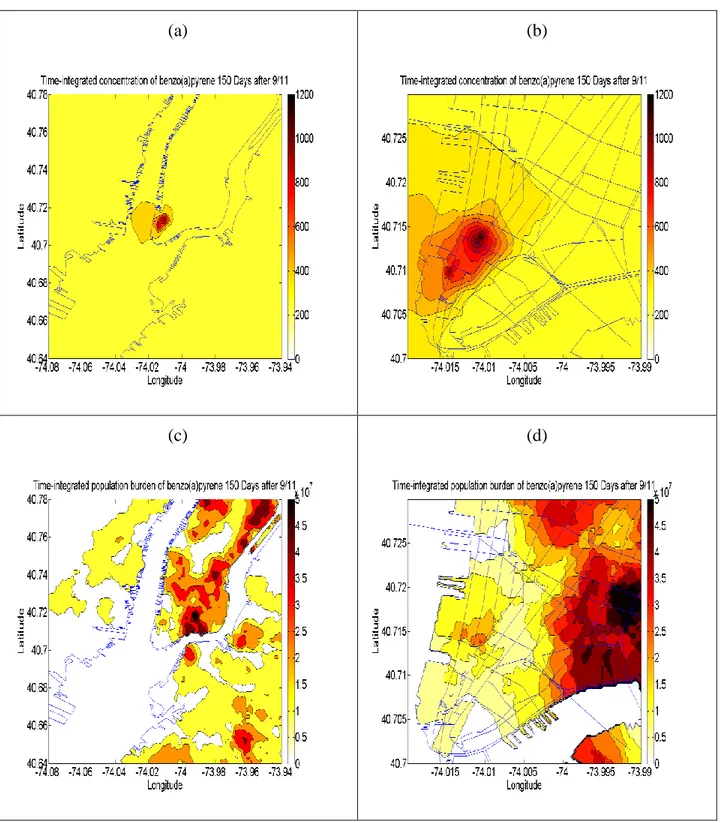
Figure 1.5 – Time-integrated concentration and population burden of benzo(a)pyrene 150 days after 9/11………...………23
Figure 2.1 – Raw distance to source relationship for H2S around hog CAFOs………...………44
Figure 2.2 – H2S LUR model restricted to “edge” field………46
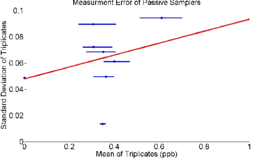
Figure 2.3 – Measurement error model for H2S……….……...…………47
Figure 2.4 – Covariance model for H2S – LUR offset………...48
Figure 2.5 – Maps of H2S concentration using different methodologies………...…………50
Figure 2.6 – Comparison of mean squared error for methods estimating H2S………...………51
Figure 3.1 – Syphilis and gonorrhea long-term vs. short term rate models………...………74
Figure 3.2 – Syphilis and gonorrhea incidence rate in North Carolina for January 1, 2009 – July 1, 2009 using BUMBME………....76
Figure 3.3 – MSE reduction relative to simple kriging for syphilis and gonorrhea using asymptotic validation………...………77
Figure 3.4 – Observed and estimated syphilis and gonorrhea over time………...…………79
Figure 4.1 – Syphilis and gonorrhea outbreak maps………...….100
xi
LIST OF ABBREVIATIONS
AIRS Aerometric Information Retrieval System BME Bayesian Maximum Entropy
BUMBME Bayesian Uniform Model extension of BME CAFO concentrated animal feeding operation CBG census block group
H2S hydrogen sulfide
MEM measurement error model MSE mean squared error
PAH polycyclic aromatic hydrocarbon PDF probability density function PM particulate matter
ROC receiver operating characteristic STI sexually transmitted infection STRF space/time random field
1
INTRODUCTION
Point sources are defined in the context of environmental science as single identifiable locations that emit pollution into the environment. From a modeling perspective, they are “ground zero” - where a contaminant originates or is at a distance of 0 from the source. The prototypical point source of pollution is a power plant that sends particulate into the air through a smokestack. The concentration of particulate is highest near the source and it decreases with distance as it disperses into the surrounding environment. Point sources are desirable from the standpoint of mitigation strategies because the pollutant being produced must only be brought under control at the location of release.
Estimating the distribution of a given variable across space is often done with traditional geostatistics, such as the simple kriging method, which estimates the variable at unmeasured locations by weighting measurements within a neighborhood of that location according to a covariance model. This method can easily be extended to space/time so that estimates can be produced as the variable changes over time. With the development of modern geostatistical methodologies, such as Bayesian Maximum Entropy, Gaussian and non-Gaussian distributions of error can be incorporated into spatiotemporal models, producing better estimates.
2
monitors to expand the number of estimated PAH measurements. The second part of the thesis examines a situation where many point sources across space contribute to pollution. The pork industry changed dramatically in the 1980s and 1990s, replacing traditional hog farms with industrial operations which house hundreds or thousands of swine, store the waste in pits, and then spray it onto land to drain the pits. In order to estimate the hydrogen sulfide concentration in a community affected by a high density of these operations, passive samplers were placed to record two week average measurements. These values were used to create a land use regression model and then to produce geostatistical estimates that include a non-Gaussian measurement error model. The final two chapters investigate an unorthodox “point source” by attempting to identify core areas – locations with elevated rates that perpetuate an infection – of syphilis and gonorrhea in North Carolina. To locate these “sources,” which have the ability to move in space and time, a Bayesian-derived non-Gaussian model for the error is used to improve estimation of incidence rates on a fine space/time scale. These estimates are then incorporated into an outbreak detection algorithm so that a source of infection can be controlled or eliminated before it
3 CHAPTER 1
A SINGLE SOURCE – UTILIZING PM2.5 AS SECONDARY INFORMATION FOR MAPPING ATMOSPHERIC POLYCYCLIC AROMATIC HYDROCARBONS
FOLLOWING THE COLLAPSE OF THE WORLD TRADE CENTER
Overview
On September 11, 2001, terrorists crashed airplanes into the two main World Trade Center towers, located in the lower Manhattan section of New York City, causing the buildings to collapse. The fires that ensued in the following days and the large amount of diesel equipment needed to clean-up the area created a point source of polycyclic aromatic hydrocarbons (PAHs), pollutants which have been classified as carcinogenic and teratogenic, in the middle of a major population center. These pollutants, which are a component of PM2.5, were measured in PM2.5 samples in the area immediately around where the towers collapsed. The mass fraction of PAH to PM2.5 was used to estimate PAH across a larger spatial domain and this method was compared to the traditional simple kriging method that only used actual PAH measurements. From a public health perspective, it is important to characterize the exposure to this pollutant since it was in the middle of a major metropolitan area and affected a large number of people, since the
4 1.1 Introduction
Extensive research has been conducted on effects resulting from exposure to ambient particulate matter. Particulate matter has been linked to cardiovascular diseases, respiratory problems, and reproductive effects. A large body of work on particulate matter focuses on atmospheric particles less than 10 microns in size (PM10); more recently, research has been extended to investigation of fine particulate matter (particles less than 2.5 microns in
aerodynamic diameter, PM2.5), which travel deeper into the lungs and increase the risks of health effects. The overwhelming evidence that high concentrations of atmospheric particulate matter (PM) are associated with adverse health effects led the United States Environmental Protection Agency (EPA) to create the Aerometric Information Retrieval System (AIRS) in order to document ambient PM levels for purposes of data storage, retrieval, and interpretation. This is a nationwide system of stations that typically monitor daily concentrations of PM. Since the effects of exposure to this criteria pollutant are well established, research is starting to focus on what compounds in the PM drive the associations.
One class that could be contributing to adverse health outcomes is polycyclic aromatic hydrocarbons (PAHs). PAHs are produced by incomplete combustion during the process of burning fossil fuels (Caricchia et al. 1999). Many of these compounds have been classified as carcinogenic, mutagenic, and teratogenic by U.S. EPA
(http://cfpub.epa.gov/ncea/iris/index.cfm) and IARC (http://monographs.iarc.fr/). Sixteen are identified as representative of this class by the EPA. Nine of these 16 are typically particle-bound compounds and were the focus of this study: benz(a)anthracene, chrysene,
benzo(b)fluoranthene, benzo(k)fluoranthene, benzo(a)pyrene, indeno(1,2,3-c,d)pyrene,
5
particles, they make up a fraction of the PM collected by filters from the EPA AIRS monitors (Guo et al. 2003; Vardar and Noll 2003). The toxicity of these compounds relative to
benzo(a)pyrene can be found in Table 1.1.
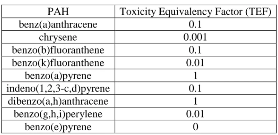
Toxicity equivalency factors for particle-bound PAHs PAH Toxicity Equivalency Factor (TEF)
benz(a)anthracene 0.1
chrysene 0.001
benzo(b)fluoranthene 0.1
benzo(k)fluoranthene 0.01
benzo(a)pyrene 1
indeno(1,2,3-c,d)pyrene 0.1
dibenzo(a,h)anthracene 1
benzo(g,h,i)perylene 0.01
benzo(e)pyrene 0
Table 1.1 Toxicity equivalency factors for particle-bound PAHs relative to benzo(a)pyrene.
Although PAHs are identified as carcinogens, non-cancerous endpoints also show
associations with these compounds. These include reproductive and developmental effects due to fetal PAH exposure (Perera et al. 2002; Berkowitz et al. 2003; Landrigan et al. 2004; Lederman et al. 2004; Miller et al. 2004; Tonne et al. 2004; Bocskay et al. 2005; Wolff et al. 2005).
6
The reproductive outcome of intrauterine growth restriction (IUGR), which has been linked to developmental problems, has also shown associations with exposure to PAHs
(Berkowitz et al. 2003). Previous studies suggested that there might be a link between IUGR and PM. One study, however, compared areas with similar PAH concentrations and different levels of particles, finding the rate of IUGR was comparable. This suggests that PAHs, not PM, could be the pollutant of concern (Dejmek et al. 2000).
The collapse of the World Trade Center (WTC) and other buildings in its immediate area on September 11, 2001 produced a large plume of dust and gases that was visible for miles around over a period of several days. The dust and debris of crushed building materials from the collapse of the towers blanketed the lower Manhattan area. Although large particles were in the majority, the smaller particles that have the ability to travel deep into the lungs are of greatest concern (Fagan et al. 2002). It has been estimated that 11,000 tons of PM2.5 were emitted into the air around the area. This included high concentrations of particle-bound PAHs (Lioy et al. 2002; Christen 2003; Edelman et al. 2003; McGee et al. 2003; Swartz et al. 2003; Wolff et al. 2005).
The immediate source of PAHs at the WTC site was burning jet fuel from the two planes that crashed into the towers. Subsequently, the primary source shifted to the fires that continued burning up to 100 days after the terrorist attacks. The fuel that produced these fires was
7
approximately 150 days after the towers’ collapse. After this time, PAHs in the area began to return to background concentrations (Pleil et al. 2004a).
Given that PAHs are possibly associated with several adverse health outcomes and the WTC collapse was a large source of these compounds, it is important to characterize the
population’s exposure to PAHs following 9/11. Since exposure changes based on the space/time point where an individual is located, it is necessary to produce space/time maps for fully
describing concentrations. This is typically conducted by measuring the pollutant at certain space/time points and using this data to interpolate values at unmeasured locations. Specific measurements for PAHs are not performed routinely as they are not part of the National Ambient Air Quality Standards (NAAQS) monitoring requirements, but instead are performed only
episodically at few locations for specific assessment projects. As such, developing the link between PAHs and the more available PM2.5 data is an important exposure and risk assessment tool.
PM2.5 samplers from the AIRS network were in the New York area before 9/11, and the EPA installed four additional samplers for measuring particulate matter specifically around Ground Zero. A new method had previously been developed at EPA for assessing particle bound PAHs from PM2.5 filters (Pleil et al. 2004b) and was applied to the archived filters from the four additional stations, producing a small amount of particle-bound PAH data.
8 1.2 Methods
1.2.1 Sampling
The EPA placed air samplers for a variety of species in lower Manhattan after the collapse of the WTC. Filters from four of the ambient PM2.5 samplers were archived and later tested for particle bound PAHs. The nine representative PAHs were benz(a)anthracene, chrysene, benzo(b)fluoranthene, benzo(k)fluoranthene, benzo(a)pyrene, indeno(1,2,3-c,d)pyrene,
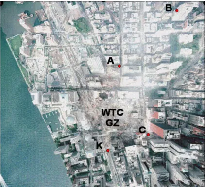
dibenzo(a,h)anthracene, benzo(g,h,i)perylene, and benzo(e)pyrene. Three of the samplers (A,C,K) were located at ground level immediately around Ground Zero (as close as the fence would allow), and the fourth sampler (B) was placed on the 16th floor of a building that was approximately 1 km from the site of the towers (Figure 1.1). This method produced daily averages for each of the nine PAHs from September 22, 2001 until March 27, 2002. The space/time locations of these samplers are referred to as phard, because particle-bound PAHs at these locations are measured without noticeable errors.
9
Locations of PAH samplers near Ground Zero
Figure 1.1 Samplers A, C, and K were placed around the fence line of Ground Zero. Sampler B was located about 1km away on the 16th floor of the EPA building.
1.2.2 Mass Fraction Model for WTC PAHs
The mathematical formulation of the mass fraction spatiotemporal geostatistics model for
particle-bound compounds can be found in Appendix A.
The log-mass fraction (log-MF) whard,iat each space/time location pi phard was calculated using the following formulae:
whard,i = ln(PAHhard,i(ng/m3) / PM2.5hard,i (μg/m3)) (1.1)
10
A6 and A7), using a space/time distance d(pi,pj) D that corresponds to a 60-day moving window with a spatial radius encompassing 10 km around each point pj (i.e. d(pi,pj) =||si-sj|| if |t
i-tj|30 days, d(pi,pj) =inf. otherwise, and D=10 km).
The estimated mean and variance of the log-MF were used to derive a soft log-PAH datum from each measured log-PM2.5 value (Eqs. A8 and A9). This produced a Gaussian PDF (Eq. A10) describing the uncertainty in the soft data for log-PAHs at the soft data points pj psoft.
The use of the AIRS PM2.5 data allows us to extend the geographic area over which PAHs can be estimated. In the WTC application of this model, the PAH data is only available near the WTC site, while the PM2.5 data is available over a much wider area. In order to address this data limitation we limited the AIRS PM2.5 stations used to be within D=10 km of the WTC site. The 10km radius contains a high density of tall buildings, similar to that around the WTC site. We believe that a larger radius would include areas where winds are not blocked by buildings and that PAH and PM2.5 would behave differently than around the WTC. This
constraint offers a mechanism to ensure that the PM2.5 stations used were within the same overall air shed as the WTC site where fires and other typical urban sources are present. However, this constraint can be relaxed for other applications where PAH data is not limited spatially as long as there are sufficient hard data to establish the ratios.
1.2.3 Space/Time Mean Trend and Covariance
11
function for each of the nine compounds. This global mean trend function was obtained using an empirical procedure that provides the benefit of using information provided by the data, and leads to a model with realistic physical characteristics of the plume. We used an additive separable space/time function for this global mean trend.
The spatial component was calculated empirically by averaging the log-PAH values at each monitoring station over the study period. These averages were smoothed using an
exponential filter with a moving window radius that increases with the distance from the WTC site. This method served two purposes. It put more weight on the directly measured log-PAH values located at the WTC, and it created a physically realistic plume-like spatial component centered at the WTC site that is known to have existed from aerial photography evidence after the towers collapsed. The temporal component was calculated using a previous model developed for PAHs at the WTC site. One should refer to the article by Pleil et al. (2004a) for an in-depth description of this temporal component.
The effect of the additive space/time mean trend function in log space is a PAH plume centered at the WTC that flattens over time, slowly returning to its pre 9/11 background concentration. This space/time mean trend was removed from the hard and soft log-PAH data, with geostatistical estimation procedures (Christakos 1990, 2000) conducted on the residuals.
12
1.2.4 Concentration Mapping and Exposure Estimates
The Bayesian Maximum Entropy (BME) framework (Christakos 1990, 2000) was used to process the general knowledge (ie. mean and covariance), hard data (i.e. directly measured) and soft data (i.e. estimated from mass fraction) for the residual log-PAH field, and to obtain a posterior PDF characterizing the residual log-PAH concentration at estimation points distributed across space and time in the New York/New Jersey area. The median PAH concentration and the lower and upper bound of the 68% confidence interval are obtained by adding back the global mean trend and back transforming the corresponding statistical estimator for the residual log-PAH.
The numerical implementation of this work was done using the BMElib package (Serre and Christakos 1999; Christakos et al. 2002) written in MATLABTM. The library makes it easy to integrate the general and site specific knowledge bases developed in this work, and to obtain the BME median estimate of PAH concentrations. Readers are referred to Appendix A for a thorough description of the BME framework.
Two types of maps were then constructed to display the PAH concentrations following the WTC disaster. The first type of map is an aggregate estimate of the concentration that one would be exposed to at a given point for a given residence time. The second type of map calculates a potential population burden that accounts for population density.
Specifically, the time-integrated PAH concentration can be calculated as:
Time Integrated PAH Concentration = (Σ PAH)*(DAI)*(TEF) (1.2)
13
DAI is the daily air intake (assumed to be 11m3/day for a person at rest), and TEF (unitless) is the toxicity equivalency factor relative to benzo(a)pyrene. These maps show the geographic areas that had the highest PAH concentrations following 9/11 after normalizing to the toxicity of benzo(a)pyrene.
The maps for potential population burden are created by multiplying the time integrated PAH concentration by the population density. They are calculated using equation (1.3), where
PD (persons/mi2) is the population density:
Time Integrated PAH Population Burden = (Σ PAH)*(DAI)*(TEF)*(PD) (1.3)
These maps show the population impact of PAH concentrations. Areas with higher population density show a higher population burden compared to a similar time integrated PAH concentration, but lower population density.
1.2.5 Validation
Validation was performed to check the performance of the mass fraction model. This was done using two methods: a spatial validation and a temporal validation. To validate the mass fraction model in space, the hard data from one of the Ground Zero monitoring stations measuring co-located PAHs and PM2.5 were removed and re-estimated by the mass fraction model. Then PAHs derived from PM2.5 were compared to the space/time kriging model that only used the directly measured PAH information. Reduction of the mean squared error (MSE)
directly-14
measured PAH data from days not removed and PAH data derived from PM2.5. This was
compared to space/time kriging, which generated estimates based on PAH values from days not removed. The reduction in the relative MSE was again the measure of success.
1.3 Results
1.3.1 Exploratory Analysis
An exploratory analysis of the data was conducted to get a sense of the behavior throughout space and time. The statistical distributions for each of the nine PAHs of interest were highly skewed from normality, as expected for this type of environmental data, and a log transformation was therefore implemented.
15
available. All PAHs show higher values at monitoring stations A,C, and K (those closest to Ground Zero) and lowest values at station B (290 Broadway, approximately 1km away). Because PM2.5 was the basis for the creation of soft PAH information at unmeasured space/time locations, it is important to characterize its behavior near the WTC site as well. Predictably, the temporal trend is very similar to that of PAHs. PM2.5 displays high variability over the study period with a decrease in concentration over time. The values reflect higher concentrations compared to the time series of PAHs since the PAHs make up a fraction of the PM2.5 mass.
1.3.2 Mass Fraction Model
The co-located PAH and PM2.5 data were used to model the log-MF of PAH to PM2.5. The estimated distribution of the log-MF for each PAH compound was derived from the 60-day moving window approach described previously. A 60-day moving window was used to capture a more realistic estimate of the behavior at unmeasured locations due to the high temporal
16
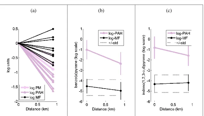
Spatial variability of log PAH, log PM2.5, and log MF
(a) (b) (c)
Figure 1.2 (a) The change in mean by distance (using the WTC sites as a baseline) for log PM, log PAH and log MF for all 9 PAH compounds. (b) The vertical bars at distance 0km (WTC sites) and 0.9km (Station B) represent the mean +/-one standard deviation for the
log-transformed benzo(a)pyrene data and its corresponding mass fraction collected at those
respective monitoring locations. The horizontal dotted line depicts +/- one standard deviation of the mass fraction mean based on the pooled data. (c) Similarly, this is shown for the compound indeno(1,2,3-c,d)pyrene.
17
are easily contained within one standard deviation of their respective mass fraction mean based on the pooled data. If we can assume that the enrichment of PAHs in PM2.5 is due to the same source at the WTC, then there is no evidence to reject that the slope of the spatial gradient with respect to the mass fraction is different from 0 within a reasonable distance of the source. Therefore, our mass fraction model that is used to derive soft PAH data from surrounding PM2.5 stations is based on the assumption that the MF is homogenous across space, while decreasing as the number of days from 9/11 increases.
The log-MF data points tend to be within one standard deviation of the estimated mean for the model, showing that the 60-day moving window is a reasonable method to use. One notable exception is the compound dibenzo(a,h)anthracene, which has a set of values that consistently lie well below the expected distribution. Therefore, soft data created for this PAH tends to be less reliable than others. We observed that in general, this PAH is present at lower absolute value than the other target compounds and is therefore more difficult to measure.
These log-MF distributions were used to derive the soft data for log-PAH concentrations from PM2.5 measurements at EPA AIRS monitoring stations from the New York metropolitan area. Using the soft data from these additional stations allowed for an increased spatial domain that covered lower Manhattan and surrounding areas.
1.3.3 Space/Time Mean Trend and Covariance
18
data available for the homogenous/stationary residual field. The shape of this global mean trend is a plume with its peak at Ground Zero on September 11, 2001. As time increases from day 0 (9/11), the plume decreases while spreading over space.
The data of the homogenous/stationary residual field were then used to obtain estimates of covariance for various spatial and temporal lags. The data used in this estimation included the hard values from the WTC as well as the mean of the log-PAH distribution of residuals derived from PM2.5. Use of the soft data was necessary to have a covariance that described the
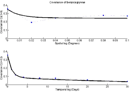
dependence between two points at distances greater than the small spatial extent covered by the WTC data. Nested exponential/exponential space/time separable covariance models produced the best fit to the data for all nine PAHs (Eq. 1.4).
2 1 3 2 2 2 1 1 1 3 exp 3 exp 3 exp 3 exp 3 exp 3 exp ) , ( t r t r t r X a a r c a a r c a a r c r
c (1.4)
where r and τ are the spatial and temporal lags, respectively, between space/time points, the ar. are spatial ranges, and the at. are temporal ranges. The parameters fit to this model for each of the nine PAHs are shown in Table 1.2, and the typical shape of the spatial and temporal components are illustrated by the covariance model for benzo(a)pyrene (Figure 1.3).
Covariance model parameters for each PAH
PAH c1 c2 c3 ar1 ar2 at1 at2
19
Covariance model for benzo(a)pyrene
Figure 1.3 Nested exponential/exponential space/time separable covariance model for benzo(a)pyrene
1.3.4 Comparison of Methods
The estimation of PAHs using BME with soft data was compared to the alternative of space/time kriging using only hard PAH data. Space/time kriging was considered the best possible method available that does not use the additional information from PM2.5. Spatial and temporal validations were conducted in order to compare the two methods. Both comparisons showed a reduction in MSE when the soft PAH data was included in the estimation.
20
away from the WTC, thereby providing a greater opportunity for contrast between the two methods. Although this still only represented a small area for showing the estimation
improvement when using soft data, we presume that as distance from the WTC increases, one could expect that the contrast between methods would further increase, leading to a larger reduction in MSE.
Spatial and temporal validation of BME vs. kriging
(a) (b)
Figure 1.4 (a) The spatial validation showing reduction in the MSE using BME compared to space/time kriging. The number for PAH refers to: 1) benz(a)anthracene, 2) chrysene, 3) benzo(b)fluoranthene, 4) benzo(k)fluoranthene, 5) benzo(a)pyrene, 6)
indeno(1,2,3-c,d)pyrene, 7) dibenzo(a,h)anthracene, 8) benzo(g,h,i)perylene, and 9) benzo(e)pyrene. (b) The temporal validation showing reduction in the MSE for benzo(a)pyrene.
21
dramatic effect than the spatial validation. All nine PAHs showed similar trends to that of benzo(a)pyrene (Figure 1.4b). This illustrates the importance of the mass fraction model for obtaining information about PAHs from available PM2.5 data when only sparse PAH data is available.
1.3.5 Exposure Mapping Results
The availability of PM2.5 data across the New York metropolitan area allowed concentration maps to be created that incorporate the soft PAH information. Maps were constructed for each day in the study period and made into a movie. However, the daily PAH maps are highly variable and not as informative as maps aggregated over time. Hence we map the time-integrated PAH concentration (Eq. 1.2) to characterize the areas of New York that were most affected by the higher levels of PAHs in the atmosphere. The time-integrated PAH
concentration for benzo(a)pyrene 150 days after 9/11 is shown in Figures 1.5a and 1.5b. The areas of highest time-aggregated PAH concentrations are those around Ground Zero and the areas to the south and west. These maps show that a hypothetical person at rest with average lung capacity standing at Ground Zero would have inhaled over 1000 ng of
22
As mentioned earlier, there are no reliable hard data for the first 10 days after 9/11
because the main focus was on human rescue efforts and sampling sites were not yet established. We expect that workers in the area likely experienced higher inhalation exposures than the general public as they were typically doing difficult tasks requiring higher pulmonary ventilation rates. This issue is beyond the scope of this work, but has been addressed in other publications contrasting the public with firefighters, rescue workers, cleanup crews, construction and
sanitation workers (Dahlgren et al. 2007; Herbert et al. 2006; Fireman et al. 2004; Lorber et al. 2007; Landrigan et al. 2004).
Including residential population density shows a different picture for the potential effect of PAHs. These maps can help estimate the population/economic burden resulting from elevated PAH levels. Multiplying the residential population density by the time integrated concentration (Eq. 1.3) produces the maps of residential population burden shown in Figures 1.5c and 1.5d. Since Ground Zero and areas west are typically non-residential areas, these places do not show high levels of residential population burden. The highly populated residential area of eastern lower Manhattan had the greatest population based exposure based on these calculations. Similarly, highly populated areas east and west of Central Park although with lower
23
Time-integrated concentration and population burden of benzo(a)pyrene 150 days after 9/11
(a) (b)
(c) (d)
24
The residential population density maps represent where the population resides during non-working hours. If daytime population densities were available, a much different map would emerge. The financial district (around the WTC site), for example, could display the highest population burden during the daytime hours due to its high density of office buildings but this would require additional information regarding infiltration and ventilation rates.
1.4 Discussion
This research produces the first maps to date displaying estimates of the space/time concentrations and variability of increased PAH levels after the collapse of the WTC. Using the limited amount of PAH data available, a mass fraction approach to producing soft PAH data made it possible to extend the geographical area covered by the PAH maps.
The maps of PAHs in lower Manhattan from this study provide advanced atmospheric concentration estimates for these pollutants not available in previous studies concerning health outcomes due to the environmental air pollution from the WTC. Other measures for WTC PAH contributions include the visible plume of debris and the number of PAH-DNA adducts.
However, neither of these methods captures the comprehensive nature of PAH exposure for individuals in the New York area following 9/11. Our space/time maps allow for the integration of daily PAH and PM2.5 data to estimate time-integrated PAH concentrations that provide a measure for ecologic exposure assignments.
25
help determine their indoor PAH exposure. Our maps created for outdoor exposure cannot account for these factors and could underestimate or overestimate based on how an individual spends their time.
As mentioned earlier, directly measured PAH data are not available for the 10 days immediately following the towers’ collapse due to the logistics of the disaster response and rescue. Using a regression model developed previously, an estimate of these compounds was included for these days as well (Pleil et al. 2004a). However, we cannot validate our model during this period without hard PAH data. This likely causes under-prediction in our PAH exposure maps as the mass fractions of PAHs were likely higher during these initial days than the value estimated starting on day 10.
Finally, the maps regarding the population impact due to PAHs refer to population estimates where people live, not where they work. Although detailed information regarding where people spend their workday were not available to us, many New Yorkers typically spend the majority of their day within a relatively small distance from their home. Therefore, the maps of population impact can generally show where the most people would likely encounter PAHs. If detailed information about how one spends their day were available, these maps could be refined to characterize their exposure.
Research studies have confirmed that exposures to fine particulate matter as a whole are related to a variety of adverse health outcomes without specific regard to their precise
composition. This work provides an additional tool for deducing PM2.5 effects by considering the enrichment of the particles with PAHs which, as a group, demonstrate carcinogenic,
26
play an integral part of this research in order to conduct large studies where the use of personal samplers is impractical.
The mass fraction approach for estimating PAH concentrations from archived PM2.5 samples has several benefits over the traditional geostatistical method of space/time kriging using only directly-measured PAH data. Our method allows for greater spatial and temporal coverage in an exposure assessment for PAHs. The additional cost is only a function of the number of PM2.5 samples analyzed and not the need for more, expensive monitors. By creating a parametric model based on this method, it may become possible to predict PAH concentrations using weather and readings of other atmospheric pollutants. This would reduce additional costs to virtually zero. In addition to the approach developed here for a massive, but transient event, future work should also focus on long-term ambient exposures as produced by numerous smaller point sources (factories, incinerators, refineries, forest fires, agricultural burning), long range transport of PM2.5, and distributed or line sources (vehicle traffic in congested urban areas, busy highways, ship channel traffic, airports). There are several reasons why the mass fraction method could perform even better under these circumstances. In contrast to the high variability of WTC aftermath where fires continuously flared up and diminished, PAH and PM2.5
27
However, it is difficult to predict how our approach will perform elsewhere. While a large amount of these pollutants were produced in the disaster, this dataset had a very limited spatial domain which included only four monitoring stations around the immediate WTC area. This left a small spatial area in which to perform the validation procedure. While it is possible this inflated the performance of our method, the station used for validation recorded PAH values that were consistently an order of magnitude lower than those around the WTC fence. Therefore, it is reasonable to assume that the method would improve if PAH data outside lower Manhattan were available for validation.
A limitation of our approach in the WTC situation is that the mass fraction model was created only using data from lower Manhattan in order to estimate concentrations outside the model’s spatial domain. While it is true that prediction reliability from PM2.5 will decrease outside of the WTC, a counterargument is that some information about PAHs from PM2.5 is much better than no information at all in these areas. The exponential shape of the temporal validation supports this hypothesis.
This application used a normal distribution to characterize the soft data at points outside Ground Zero. It would have also been possible to use the actual statistical distributions of the log-MF. This would be beneficial for those compounds whose log-MF showed an obvious departure from normality. Dibenzo(a,h)anthracene, which produced a bimodal distribution, would have been the only compound in this study that probably would have benefited from this type of analysis. Even with the challenges posed by this dataset and study area, the mass fraction method for creating additional soft PAH information appears to make considerable
28
The concept of using the mass fraction to predict PAHs from readily available PM2.5 data could become a useful regulatory or epidemiological assessment tool because there are obvious cost savings by not having to deploy special samplers and make separate PAH measurements at all space/time monitoring locations. Future data sets that include more spatially diverse PAH data would be useful in developing a better model. Applying this model to a rare disaster with many contaminants such as the WTC is a worst-case scenario for evaluation. However, despite the complexity of the dataset, the mass fraction appears to be very useful compared to traditional kriging methods. We expect that the accuracy and value of state-wide assessments, in the absence of extraordinary events, would benefit even more from these methods.
In conclusion, the mass fraction approach for creating soft data from PM2.5 appears to be a promising method for estimating concentrations of PAHs in future studies. Since the
29
REFERENCES
Berkowitz GS, Wolff MS, Janevic TM, Holzman IR, Yehuda R, Landrigan PJ (2003) The World Trade Center disaster and intrauterine growth restriction. JAMA 290(5):595-596
Bocskay KA, Tang D, Orjuela MA, Liu X, Warburton DP, Perera FP (2005) Chromosomal aberrations in cord blood are associated with prenatal exposure to carcinogenic polycyclic aromatic hydrocarbons. Cancer Epidemiol Biomarkers Prev 14(2):506-511
Caricchia AM, Chiavarini S, Pezza M (1999) Polycyclic aromatic hydrocarbons in the urban atmospheric particulate matter in the city of Naples (Italy). Atmospheric Environment 33(23):3731-3738
Christakos G (1990) A Bayesian maximum-entropy view to the spatial estimation problem. Mathematical Geology 22(7):763-777
Christakos G (2000) Modern Spatiotemporal Geostatistics. Oxford University Press, New York, NY
Christakos G, Bogaert P, Serre ML (2002) Temporal GIS: Advanced Functions for Field-Based Applications. Springer-Verlag, New York, p. 217
Christen K (2003) High PAH levels in dust from 9/11 disaster. Environ Sci Technol 37(3):49A-50A
Dahlgren J, Cechini M, Takhar H, Paepke O (2007) Persistent organic pollutants in 9/11 world trade rescue workers: reduction following detoxification. Chemosphere 69(8):1320-1325
Dalton L (2003) Chemical analysis of a disaster. Chemical Engineering News 81(42):26-30
30
Edelman P, Osterloh J, Pirkle J, Caudill SP, Grainger J, Jones R, et al. (2003) Biomonitoring of chemical exposure among New York City firefighters responding to the World Trade Center fire and collapse. Environ Health Perspect 111(16):1906-1911
Fagan J, Galea S, Ahern J, Bonner S, Vlahov D (2002) Self-reported increase in asthma severity after the September 11 attacks on the World Trade Center--Manhattan, New York, 2001.
MMWR Morb Mortal Wkly Rep 51:781-784
Fireman EM, Lerman Y, Ganor E, Greif J, Firemean-Shoresh S, Lioy PJ, et al. (2004) Induced sputum assessment in New York City firefighters exposed to World Trade Center dust. Environ. Health Perspect 112(15):1564-1569
Guo H, Lee SC, Ho KF, Wang XM, Zou SC (2003) Particle-associated polycyclic aromatic hydrocarbons in urban air of Hong Kong. Atmospheric Environment 37(38):5307-5317
Herbert R, Moline J, Skloot G, Metzger K, Baron S, Luft B, et al. (2006) The Word Trade Center Disaster and the health of workers: five-year assessment of a unique medical screening program. Environ. Health Perspect 114(12):1853-1858
Landrigan PJ, Lioy PJ, Thurston G, Berkowitz G, Chen LC, Chillrud SN, et al. (2004) Health and environmental consequences of the World Trade Center disaster. Environ Health Perspect 112(6):731-739
Lederman SA, Rauh V, Weiss L, Stein JL, Hoepner LA, Becker M, Perera FP (2004) The effects of the World Trade Center event on birth outcomes among term deliveries at three lower
Manhattan hospitals. Environ Health Perspect 112(17):1772-1778
Lioy PJ, Weisel CP, Millette JR, Eisenreich S, Vallero D, Offenberg J, et al. (2002)
Characterization of the dust/smoke aerosol that settled east of the World Trade Center (WTC) in lower Manhattan after the collapse of the WTC 11 September 2001. Environ Health Perspect 110(7):703-714
Lorber M, Gibb H, Grant L, Pinto J, Pleil J, Cleverly D (2007) Assessment of inhalation exposures and potential risks to the general population that resulted from the collapse of the World Trade Center Towers. Risk Analysis 27(5):1203-1221
31
Emergency Management Agency Report 403. Federal Emergency Management Agency, Washington, DC
McGee JK, Chen LC, Cohen MD, Chee GR, Prophete CM, Haykal-Coates N, et al. (2003) Chemical analysis of World Trade Center fine particulate matter for use in toxicologic assessment. Environ Health Perspect 111(7):972-980
Miller RL, Garfinkel R, Horton M, Camann D, Perera FP, Whyatt RM, Kinney PL (2004) Polycyclic aromatic hydrocarbons, environmental tobacco smoke, and respiratory symptoms in an inner-city birth cohort. Chest 126(4):1071-1078
Nordgren MD, Goldstein EA, Izeman, MA (2002) The environmental
impacts of the World Trade Center attacks: a preliminary assessment. National Resources Defense Council, New York
Perera F, Hemminki K, Jedrychowski W, Whyatt R, Campbell U, Hsu Y, et al. (2002) In utero
DNA damage from environmental pollution is associated with somatic gene mutation in newborns. Cancer Epidemiol Biomarkers Prev 11(10):1134-1137
Perera FP, Rauh V, Tsai W, Kinney P, Camann D, Barr D, et al. (2003) Effects of transplacental exposure to environmental pollutants on birth outcomes in a multiethnic population. Environ Health Perspect 111(2):201-205
Perera F, Tang D, Whyatt R, Lederman SA, Jedrychowski W (2005) DNA damage from polycyclic aromatic hydrocarbons measured by benzo[a]pyrene-DNA adducts in mothers and newborns from northern Manhattan, the World Trade Center area, Poland, and China. Cancer Epidemiol Biomarkers Prev 14(3):709-714
Pleil JD, Vette AF, Johnson BA, Rappaport SM (2004a) Air levels of carcinogenic polycyclic aromatic hydrocarbons after the World Trade Center disaster. PNAS 101(32):11685-11688
Pleil JD, Vette AF, Rappaport SM (2004b) Assaying particle-bound polycyclic aromatic hydrocarbons from archived PM2.5 filters. Journal of Chromatography A 1033(1):9-17
32
Puangthongthub S, Wangwongwatana S, Kamens RM, Serre ML (2007) Modeling the space/time distribution of particulate matter in Thailand and optimizing its monitoring network. Atmospheric Environment 41(36):7788-7805
Serre ML, Christakos G (1999) Modern geostatistics: Computational BME in the light of uncertain physical knowledge--The Equus Beds Study. Stochastic Environmental
Research and Risk Assessment 13(1):1-26
Serre ML, Christakos G, Lee S (2004) Soft data space/time mapping of coarse particulate matter annual arithmetic average over the U.S. In: Sanchez-Vila X, Carrera J, Gomez-Hernandez JJ (eds) geoENV IV-Geostatistics for Environmental Applications. Springer, New York, pp. 115-126
Swartz E, Stockburger L, Vallero DA (2003) Polycyclic aromatic hydrocarbons and other semivolatile organic compounds collected in New York City in response to the events of 9/11. Environ Sci and Technol 37(16):3537-3546
Tonne CC, Whyatt RM, Camann DE, Perera FP, Kinney PL (2004) Predictors of personal polycyclic aromatic hydrocarbon exposures among pregnant minority women in New York City. Environ Health Perspect 112(6):754-759
Vardar N, Noll KE (2003) Atmospheric PAH concentrations in fine and coarse particles. Environmental Monitoring and Assessment 87(1):81-92
33 CHAPTER 2
MULTIPLE SOURCES IN SPACE – USING LAND USE REGRESSION TO ESTIMATE ATMOSPHERIC HYDROGEN SULFIDE IN AN AREA WITH A HIGH DENSITY OF
INDUSTRIAL HOG OPERATIONS
Overview
Pork production in the United States has moved to an industrial model where a large number of swine are confined in a building. The waste from the hogs in these buildings is captured and sent to a holding pit that must be pumped out periodically. In North Carolina, the waste is often sprayed on adjacent fields. While this method of waste treatment should in and of itself cause environmental concerns, the problem is multiplied by the fact that hog operations are concentrated in rural areas of eastern North Carolina such that some counties have hundreds of these point sources of pollution. Passive samplers were placed in one such area to measure two week average concentrations of hydrogen sulfide (H2S). A land use regression model was developed to estimate the H2S concentration contributed by so many point sources within the area, and the geostatistical estimates produced were updated with a non-Gaussian measurement error model. This again was compared to the traditional method of simple kriging to quantify the improvement in estimation from using a modern geostatistical approach. Since residents
34 2.1 Introduction
During the 1980s and 1990s, hog production in North Carolina changed from a traditional model to an industrial one where swine were kept in concentrated animal feeding operations (CAFOs). A typical CAFO has buildings that can house hundreds or thousands of animals. The waste in these buildings is collected and stored in open air pits and then to maintain freeboard required by permits, most operations spray the waste on adjacent fields.
The CAFO open waste pit model has created numerous environmental concerns from contaminants in the air, water, and soil and health effects such as additional stress, irritated eyes, nose, and throat, increases in asthma, and acute blood pressure elevation (Wing et al. 2013; Mirabelli et al. 2006; Merchant et al. 2005; Bullers 2005; Hodne 2001; Wing and Wolf 2000; Cole et al. 2000; Thu et al. 1997; Schiffman et al. 1995). In addition to adverse health outcomes, CAFOs can contribute to decreased quality of life, lower property values and suppressed
economic development (Thu 2002; Palmquist et al. 1997; Thu 1996; Durrenberger and Thu 1996).
In North Carolina, there are now a large number of hog CAFOs, particularly in the eastern part of the state (NCDENR 2007). This area is typically rural, with a lower
socioeconomic status and higher Black and Hispanic populations compared to the rest of the state. The highest density of these operations is in the south central part of the North Carolina coastal plain region, especially in the area of Sampson and Duplin counties. Locations in this area can have hundreds of CAFOs within a radius of just 30 km. Thus regardless of wind direction, residences are usually downwind from CAFOs at any given time.
35
by an odor similar to that of a rotten egg. H2S is produced by the anaerobic breakdown of organic matter which occurs in the pit containing hog waste as well as being emitted when that waste is dispersed. The odor threshold of H2S has been reported from 0.5-300 ppb. Exposure to H2S at moderate to high concentrations can cause eye and throat irritation, cough, and nausea, and acute exposure to very high concentrations of H2S can result in death (ATSDR 2006). Occupational exposure limits are not to exceed 20 ppm, however little is known regarding the effects of chronic low level exposure to the compound, especially in the presence of other air pollutants (OSHA 2014; ATSDR 2006).
This study was part of a larger project in which researchers partnered with a local community organization in eastern North Carolina. Pollutant data, biological samples, and residents’ own accounts of their health over time were collected to investigate the impacts of industrial hog operations on a community living with a high density of CAFOs. H2S was one exposure of interest in this study because accurate estimates of its concentration in space and time could be used to correlate with health effects reported by residents. While three single point monitors (SPMs) were available to record air pollutant measurements in real-time, we
complemented these devices with Radiello H2S passive samplers to provide greater spatial coverage across the study area in a cost-effective manner (Pavilonis et al. 2013; Radiello 2007). In this study, we use the average H2S concentrations collected by the passive samplers to develop a land use regression (LUR) model to indicate whether CAFOs are the source of H2S in the study area, and we then conduct a comparison of methods to find which one produces the most
36 2.2 Materials and Methods
2.2.1 Sampling
We deployed 67 Radiello passive samplers designed to collect H2S at 53 unique
space/time locations from January to June 2007. The leadership of our partner community group provided expertise regarding sampling locations and connected us with individuals who were willing to have passive samplers placed on their property. Each passive device was placed approximately 1.5-2.0 meters above the ground (breathing height) during one of six 2-3 week sampling phases. The coordinates of each passive sampler’s spatial location were recorded with a Global Positioning System (GPS). Placement of passive samplers was designed to estimate several types of variability including device measurement error and the changes in H2S concentration over space and time.
H2S sampling locations by type Sampling Phase Number Number of Unique S/T Measurements
Triplicate* Single Edge Field Blanks
1 8 5 0 3 1
2 11 2 4 5 1
3 5 0 0 5 1
4 12 0 7 5 1
5 5 0 0 5 0
6 12 0 7 5 1
S/T Locations 53 7 18 28 --
Samplers 72 21 18 28 5
*Each triplicate measure represents 3 samplers in one spatial location
37
Each sampler used in the field can be categorized as a triplicate, single, edge field, or field blank (Table 2.1). Seven of the space/time sites had samplers placed in triplicate in order to quantify the sampling error. These triplicate sites, as well as the single sampler locations, were only monitored during one sampling phase and placed in reasonable proximity (within a few km) to one another for a given sampling period where residents would allow us access to their
property. There was one area where we were able to gain access to land adjacent to a CAFO waste pit. In this “edge” field, we placed devices during each of the 6 sampling periods in order to analyze the distance to source relationship as well as the changes in H2S from one period to the next. Finally, a field blank was used during the collection period of each phase to quantify any contamination during transport (except for Phase 5 when the field blank was damaged).
The lab analysis instructions provided by Radiello were followed in order to obtain the mass of sulfide ions (ug) in each sample (see Appendix B) (Radiello 2007). The mass of sulfide ions from each passive device’s corresponding field and lab blanks, which characterized any contamination during travel and analysis, respectively, were removed from this value to obtain the corrected mass of sulfide ions in the exposed sample, which we denote as Mij for the i-th sampler collected during the j-th sampling period. The average H2S concentration (ppb) for each sample (Zij) was then calculated using the average temperature (in degrees Kelvin) during the sampling time Tij (in minutes) using Eq. 2.1.
𝑍𝑖𝑗 = 1000∗𝑀𝑖𝑗 0.096∗𝑇𝑒𝑚𝑝𝑖𝑗
3.8
298 ∗𝑇𝑖𝑗
(2.1)
2.2.2 Public Data Sources
We downloaded the spatial database of CAFOs which is maintained by the North
38
select the facilities from this database listed as swine CAFOs. In addition to the latitude and longitude coordinates of these operations, information regarding the approximate number of animals and the number of lagoons was also available (NCDENR 2007).
Hourly weather data was obtained for the weather station closest to the study area that reports to the National Oceanic and Atmospheric Administration’s (NOAA) National Climatic Data Center. Available weather variables from this database include temperature, dew point, relative humidity, wind speed, wind direction, pressure, and precipitation (NOAA 2011). Since there was only one station that was reasonably close to our passive sampler locations, hourly temperature, dew point, relative humidity, pressure, and precipitation were averaged over the collection period for each respective sampling device.
2.2.3 Land Use Regression Model
A Land Use Regression(LUR) model was developed to test the hypothesis that CAFOs are a source of atmospheric H2S in the study area, to estimate the distance (or range) over which a single CAFO contributes to the H2S concentration, and to serve as a space/time offset to remove from the observed data for the purpose of geostatistical estimation (Messier et al. 2012). We denote the space/time random field (STRF) of the instantaneous H2S concentration as Y and the time-averaged concentration of H2S as Z. The variable Z is measured for passive sampler ij at spatial coordinate si = (longitudei, latitudei) and time tj+/- Tij / 2, where Tij is the length of time (in minutes) that sampler was exposed in the field. Thus, with 𝑢 ∈ (𝑡𝑗−𝑇𝑖𝑗
2 , 𝑡𝑗+ 𝑇𝑖𝑗
39 𝑍𝑖𝑗(𝒔𝒊, 𝑡𝑗) = ∫𝑡𝑗+ 𝑌(𝒔𝒊, 𝑢)𝑑𝑢/𝑇𝑖𝑗
𝑇𝑖𝑗 2 𝑡𝑗−𝑇𝑖𝑗2
. The concentration of time-averaged H2S for passive sampler
ij can then be expressed as dependent on a set of explanatory variables 𝑋𝑖𝑗(𝑚)variables so that:
𝑍𝑖𝑗 = 𝛽0+ 𝛽1𝑋𝑖𝑗(1)+ 𝛽2𝑋𝑖𝑗(2)+ ⋯ + 𝛽𝑚𝑋𝑖𝑗(𝑚)+ 𝜀𝑖𝑗 (2.2)
, where β1, …, βm are the linear regression coefficients for explanatory variables 𝑋𝑖𝑗(1), …, 𝑋𝑖𝑗(𝑚), respectively, and εij is the error term associated with the respective sample. We expect the primary explanatory variable of interest to be the sum of wind-weighted exponential decay functions (Eq. 2.3), where each individual exponential decay function represents a contribution from a surrounding hog CAFO. For passive sampler ij, the contribution of CAFO k at hour l is given a weight wijkl defined in Eq. 2.4 such that the sum of the exponentially decaying
contributions from CAFOs is equal to:
𝑋𝑖𝑗(1) = ∑ ∑ 𝑤𝑖𝑗𝑘𝑙exp (−3𝐷𝑖𝑗𝑘 𝑎𝑟 ) 𝑛
𝑘=1 ℎ𝑖𝑗
𝑙=1 (2.3)
𝑤𝑖𝑗𝑘𝑙 =1+cos (𝛼𝑖𝑗𝑘𝑙)
2 (2.4)
40
spatial range, ar, was chosen as the one which optimized the coefficient of determination (R2) of the full model. Since only one NOAA weather station was reasonably close to the study area, the non-wind weather variables do not change over space and their average over time Tij was used. The set of estimated regression coefficients (𝛽̂0, … , 𝛽̂𝑚) can be used to construct the LUR model for H2S, which for any spatial location s and time t can be expressed as:
𝐿𝑧(𝒔, 𝑡) = 𝛽̂0+ 𝛽̂1𝑋(1)(𝒔, 𝑡) + 𝛽̂2𝑋(2)(𝒔, 𝑡) + ⋯ + 𝛽̂𝑚𝑋(𝑚)(𝒔, 𝑡) (2.5)
2.2.4 Space/Time Estimation of Hydrogen Sulfide
We utilized six methods for estimating the average concentration of atmospheric H2S in the study area. The first method, which we refer to as constant mean (CM), assumes that the H2S concentration at any space/time location can be reasonably approximated by the average
concentration of all passive samplers. We utilize this method as the null hypothesis that hog CAFOs do not contribute to atmospheric H2S and there is simply a background concentration present throughout the study area. Our second method (LUR) uses the space/time LUR model (Eq. 2.5) to estimate atmospheric H2S. The model takes into account the contribution of the sources as well as the space/time varying wind direction, and the time-varying weather variables. While it uses the space/time data for the purpose of developing the global space/time LUR model, this method does not allow for geostatistical estimation where the data also serves to influence the estimation of H2S in the local space/time neighborhood of their location.
Our third and fourth methods allow for local influence from each space/time data point by using ordinary space/time kriging. Kriging is a widely-used geostatistical method that
41
the data according to a space/time covariance function. We use a global space/time offset (oij(s,t)) for each sampler value to create the H2S offset data (Xij) (Eq. 2.6).
Xij= Zij – o(si, tj) (2.6)
We then model the variability and uncertainty associated with X(s,t) using a
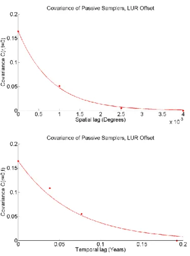
homogeneous/stationary STRF for which the set of observed values Xij represents one realization. For the third method, which we refer to as kriging-constant mean offset (K-CM), we offset each space/time data point by the average measured value of H2S as in the CM method. In the fourth method which we refer to as kriging-LUR offset (K-LUR), we offset each data point by the space/time LUR model in Eq. 2.5. A space/time separable exponential covariance model was fit to the offset data (Eq. 2.7), which captures the space/time variability of the STRF.
𝑐𝑥(𝑟, 𝜏) = 𝑐1exp (−3𝑟𝑎 𝑟1)exp (
−3𝜏
𝑎𝑡1) (2.7)
A least squares approach was used to fit a model for each offset method (CM and LUR). The kriging methods allow local influence by the measured data and assume that each measured data point is the true value of H2S and that it is measured without error (hard data).
42
detection limit and the portion of the probability density function (pdf) below the detection limit is re-normalized (Messier et al. 2012).
For the measurements above the detection limit, we created a measurement error model (MEM) that uses the field triplicates and lab and field blanks to predict the standard deviation (Wilson and Serre 2007).
𝜎𝑍𝑖𝑗 = 𝜎0+ 𝑘𝑍𝑖𝑗 (2.8)
The MEM (Eq. 2.8) shows that we expect the standard deviation of the time-averaged H2S measurement from passive sampler ij (𝜎𝑍𝑖𝑗) to be equal to the error associated with very small
values (σ0) plus a coefficient k that increases the measurement error as the measured value Zij increases. Since concentration cannot be negative, a Gaussian distribution with mean equal to the measured value (Zij) and variance given by our MEM was truncated below 0 and re-normalized. A space/time separable exponential/exponential covariance model was again fit, this time to the hardened value from our distributional (soft) data.
The Bayesian Maximum Entropy (BME) framework and its mathematical
implementation were used to process the general knowledge (ie. mean and covariance), and non-Gaussian soft data for the STRF of X and to obtain a posterior PDF characterizing X at
estimation points distributed across space and time in the study area (Christakos et al. 2002; Christakos 2000; Serre and Christakos 1999; Christakos 1990). The median H2S concentration and the lower and upper bound of the 68% confidence interval are obtained by adding back the offset for the corresponding methods used for the respective BME-CM and BME-LUR methods.
43
integrate the general and site specific knowledge bases developed in this work, and to obtain the BME median estimate of H2S concentrations.
2.2.5 Comparison of Methods
A validation was performed to compare the estimation performance among the six methods. For the non-geostatistical methods (CM and LUR), the mean squared error (MSE, defined in Eq. 2.9) for method q is calculated using the difference between the observed value (Zij) and the model estimate (𝑍𝑖𝑗∗(𝑞)) at all space/time locations where data was measured (m) by a passive sampler.
𝑀𝑆𝐸(𝑞)= 1
𝑚∑ (𝑍𝑖𝑗 ∗(𝑞)− 𝑍
𝑖𝑗)2 𝑚
𝑖𝑗=1 (2.9)
For the four geostatistical methods, each point Zij was removed from the dataset and that space/time location was re-estimated using a given method q, yielding the estimate 𝑍𝑖𝑗∗(𝑞).
2.3 Results 2.3.1 Summary
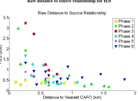
The blank-corrected measured passive sampler data (N=67) ranged from 0.17 – 3.24 ppb for average H2S concentration and the spatial distance to nearest CAFO as given by the
44
Raw distance to source relationship for H2S
Figure 2.1 The raw distance to closest source relationship (not accounting for wind or other factors) shows that H2S concentration and distance to closest CAFO are
inversely related. The strength of this relationship changes due to time-varying components and contribution from other CAFOs located further out.
2.3.2 Land Use Regression Model
Explanatory variables and their first-order interactions were included in the LUR model if they were statistically significant (α=0.05) by the stepwise inclusion/exclusion method using PROC REG in SAS Version 9.2. The resulting components of the global LUR model are given in Table 2.2. We evaluated the full LUR model for different distances of the CAFO decay range parameter ar (Eq. 2.3) ranging from 0-20 km at intervals of 0.1 km. The maximum R2 value of 0.62 occurred at a spatial range of 1.0 km. The CAFO sources (sum of wind-weighted
45
relative humidity, pressure, and precipitation were positively associated with H2S whereas dew point was negatively associated with H2S.
Statistically significant variables in H2S LUR model
Variable Coefficient F-Statistic P-Value
Intercept -268.04 (ppb) 19.71 <0.001
Unit-less Sum of Wind-Weighted Exponential Decay Functions with
ar = 1.0 km
2.64 (ppb) 40.56 <0.001
Temperature (F) 0.99(𝑝𝑝𝑏
𝐹 ) 10.53 0.0022
Dew Point (F) -1.06 (𝑝𝑝𝑏
𝐹 ) 9.49 0.0035
Relative Humidity (%) 0.58 (𝑝𝑝𝑏
% ) 6.70 0.0129
Pressure (Pa) 7.32 (𝑝𝑝𝑏 𝑃𝑎 )
12.39 0.0010
Precipitation (in) 197.10 (𝑝𝑝𝑏
𝑖𝑛 ) 8.39 0.0058
Table 2.2 The statistically significant components in the LUR model for predicting time-averaged H2S achieved an R2=0.62.
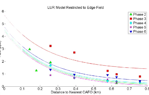
We also limited our LUR model to H2S data from the “edge” field where we were able to
place 5 samplers close to a CAFO waste pit and at increasing distances in one direction so that
the second closest operation was always at least 0.5 km further from the sampler than the target
operation. We created an “edge” model consistent with the full global LUR model, but limited to
data collected in the edge field, and accounting only for the nearest CAFO (i.e. n=1 in Eq. 2.3)
since the edge field is mainly influenced by a single operation. This helped to ascertain whether
the exponential decay function is a good model. The edge model had an R2 value of 0.80 using a
46
H2S LUR model restricted to “edge” field
Figure 2.2 The LUR model for the “edge” field which should have minimal influence from other CAFOs achieved a maximum R2 of 0.80 for a spatial range of 0.7 km. The LUR model is valid for community level exposures greater than 100m from a CAFO.
2.3.3 Distributional (Soft) Data
47
estimate the standard deviation of the distributional (soft) data. The lab and field blanks were used to obtain the value σ0 which represents the standard deviation at very low measured values of H2S and our locations where samplers were placed in triplicate were used to estimate the coefficient k which represents the increase in standard deviation as the measured value Zij increases. Given that σ0 was found to be 0.05 ppb, the least squares estimate for k was 0.05, so that we obtain the standard deviation for measurement Zij as 𝜎𝑍𝑖𝑗 = 0.05 + 0.05 ∗ 𝑍𝑖𝑗 (Figure 2.3). Using the MEM, we obtain a Gaussian distribution with a mean of Zij and variance of 𝜎𝑍2𝑖𝑗
as the distributional (soft) data used to model the uncertainty associated with each measured value above the detection limit. Each of these distributions was truncated below 0, and re-normalized, making them non-Gaussian.
Measurement Error Model for H2S