Thesis

Examining the Interior of the Llaima Volcano, Chile:

Evidence from Receiver Functions

Jordan Bishop

Honor’s Thesis

The University of North Carolina, Chapel Hill

Department of Geological Sciences

Advisor: Dr. Jonathan M. Lees

Abstract

1

The Llaima volcano is the second most active volcano in the southern Andes. However, 2

despite its frequent eruptions and close proximity to the towns of Melipueco and Vilc´un, not 3

much is known about the interior of the volcano. In 2012, a petrologic study was conducted on 4

the volcano, producing the first images of what its magmatic system is like. However, seismic 5

imaging of the interior of the volcano had yet to be conducted. In this paper, we apply receiver 6

functions to produce the first seismic study of the interior of the Llaima volcano. An iterative 7

deconvolution technique was applied to both deep local events and teleseismic earthquakes 8

recorded by seismometers near the Llaima. Once receiver functions were calculated, H-κ

9

stacking was applied to probe the Earth structure under the volcano and search for areas of 10

partial melting. From this survey, it was found that the Mohorovii discontinuity (Moho) was 11

located at approximately sixty kilometers beneath the volcano, and that a pocket of partial 12

melting was found at approximately twenty kilometers depth. This study provides the first 13

look at the deep magmatic system structure underneath Llaima. 14

1

Introduction

The Llaima volcano in Chile is one of the most active volcanoes in the world, with more than 17

50 observed eruptions since 1640 ([Naranjo and Moreno, 2005]). While many of these eruptions are 18

small, the eruption mechanics causing such frequent eruptions are unknown, and more information 19

about the crustal structure beneath Llaima is needed. 20

While many investigations have been done on the petrology and eruption history of this highly 21

active volcano, the interior of the volcano has not yet been examined using seismic imaging and 22

remains virtually unknown. In this study, we apply an iterative deconvolution technique to compute 23

receiver functions from a dense array around the Llaima volcano. By applying stacking techniques to 24

the receiver functions we attempt to provide the first seismic evidence of Llaima’s internal geometry. 25

2

Previous Work

26

2.1 Geologic Background

27

Llaima is a basaltic to basaltic-andesitic (51.0-55.7% SiO2) stratovolcano located in the Chilean

28

Southern Andes Volcanic Zone (SAVZ). Active since the late Pleistocene, the present complex, one 29

of the largest in the region (volume = 400 km3), was formed through strombolian, hawaiian, and 30

minor subplinean eruptions [Naranjo and Moreno, 1991, 2005]. 31

By examining olivine-hosted melt inclusions from four different eruptions, Maisonneuve et al. 32

[2012] concluded that magma is stored at shallow depths (≤ 4 km) beneath Llaima where it un-33

dergoes intense degassing and crystallization before eruption. A dike complex beneath Llaima was 34

Figure 1: A proposed dike complex beneath Llaima [Maisonneuve et al., 2012]

2.2 A summary of InSAR Modeling applied to Llaima

36

One of the motivations behind this thesis is a series of papers published on Llaima from 2010 37

to 2015. Fournier et al. [2010] used a combination of L band (23.6 cm) and C band (5.6 cm) radar 38

satellites in an attempt to detect deformation in volcanoes. Focusing primarily on Latin America, 39

they found deformation on the Llaima, Lonquimay, Laguna del Maule, and Cait´en volcanoes. They 40

detected an 11 cm subsidence on the eastern flank of Llaima during December 2007. Due to 41

the close proximity to the January-February 2008 eruption, it was suggested that the eruption is 42

associated with an eruption process. The authors concluded it was the result of sector collapse and 43

creep movement. It should be noted that no associated deformation was detected with the 2003 44

and 2007 eruptions at Llaima; potentially due to poor temporal or spatial modeling as a result of 45

interferogram decorrelation. 46

Bathke et al. [2011] applied a model-assisted phase unwrapping and modeling approach to noisy 47

interferograms in an attempt to characterize deformation sources. They applied this technique to a 48

similar data set at Fournier and discovered two deformation periods on Llaima: subsidence between 49

11/2003 and 05/2007 and uplift from 05/2007 to 11/2008. For both periods, they used inverse 50

modeling to determine that a magma body was located approximately 1 km to the southeast of 51

to 6-12 km and the depth of the uplift source to 4-9 km, with volume changes of 4.5−10×106

53

m3 _{and 6−20×10}6 _m3_{, respectively. They then noted that the uplift and deflation sources are}

54

possibly at to the same source due to sources of error such as 1) uncertainty with depth calculation 55

from inverse modeling (see Dawson and Tregoning [2007]) the use of a simple point source model in 56

the forward modeling, 3) upward migration of the magma during magma inflow, and 4) combined 57

magmatic and hydrothermal activity (see Battaglia et al. [2006]). 58

Three main forms of error arise when using InSAR to measure deformation on stratovolcanoes. 59

Temporal decorrelation can occur in signals due to dense vegetation, snow and ice cover, and rapid 60

gullying of sediments [Lu and Dzurisin, 2014]. Geometric distortions (foreshortening-layover) can 61

also occur due to the steep slopes of the volcano. Tropospheric chemical and physical properties 62

can also cause a changing phase delay between successive SAR images, resulting in a bias from both 63

short-wavelength and long-wavelength interferogram artifacts [Fournier et al., 2010]. In addition 64

to discussing the errors above Remy et al. [2015] noted how reliable solutions to the tropospheric 65

bias problem do not yet exist; see their paper for more details. Particularly, Remy et al. [2015] 66

analyzed the magnitude and variation of water vapor over Llaima using estimates from Medium-67

Resolution Imaging Spectrometer (MERIS) and Moderate Resolution Imaging Spectroradiometer 68

(MODIS) data, which is known to be a large source of error in InSAR imaging [Li, 2011]. As part of 69

their analysis, they used a Mogi point source model in a homogeneous elastic half-space to calculate 70

displacement vectors. The point source was placed at 7km depth to correspond with the deformation 71

source proposed by Bathke et al. [2011]. The displacement vectors were then converted to phase 72

values and compared to the interferograms. From their analysis, they cautioned the interpretation of 73

ground displacement less than±7 cm when using a single interferogram to view the entire volcanic 74

edifice. They then concluded that there was no clear evidence of ground surface displacement in the 75

2003-2011 InSAR data, and that the observed fringes are due to tropospheric effects rather than 76

ground displacements. Finally, Remy et al. [2015] postulated that the lack of coeruptive ground 77

of the sensors, displacement related to a deep source, displacement related to a very shallow source, 79

displacement confined to the incoherent peak area of the volcano, or that preeruptive inflation and 80

posteruptive deflation were observed in a single orbital cycle [Lu and Dzurisin, 2014]. 81

2.3 Receiver Function Theory

82

2.3.1 A Deconvolution Problem 83

Teleseismic receiver functions are time series derived by deconvolving the source time func-84

tion from raw seismic records on three-component seismograms [Langston, 1979]. The theoretical 85

displacement for a P-wave in the time domain is given by: 86

DV(t) = I(t)∗S(t)∗EV(t)

DR(t) =I(t)∗S(t)∗ER(t)

DT(t) = I(t)∗S(t)∗ET(t)

(2.1)

where I(t) is the instrument impulse response, S(t) is the effective source time function for the 87

earthquake, and EV(t), ER(t), and ET(t) are the impulse responses of the vertical, radial, and 88

transverse components, respectively. 89

In practice, the source time functionS(t) of the earthquake can be approximated by the vertical 90

component of the seismogram [Langston, 1977b], thereforeI(t)∗S(t)≈Dv(t). With the assumption

91

that instrument responses are matched to components,ER(t) andET(t) can then be approximated

92

by deconvolving the instrument response and source time function from the the components DR(t)

93

andDT(t). From the convolution theorem, this process is accomplished by division in the frequency

94

domain: 95

ER(ω) =

DR(ω) I(ω)S(ω) ≈

DR(ω) DV(ω)

ET(ω) =

DT(ω)

I(ω)S(ω) ≈

DT(ω)

DV(ω)

96

As noted in Langston [1979], the deconvolution in (2) may be numerically unstable due to 97

random noise and the limited bandwidth of the signal. Numerous deconvolution algorithms have 98

since been developed [Clayton and Wiggins, 1976; Oldenburg, 1981; Ligorra and Ammon, 1999; 99

Park and Levin, 2000] with both frequency-domain and time-domain approaches. In this study, we 100

calculated radial receiver functions using an iterative deconvolution technique [Ligorra and Ammon, 101

1999]. First illustrated by Kikuchi and Kanamori [1982], this technique has the advantages of 102

both constraining the spectral shape at long periods and intuitively stripping information from 103

the original signal in order of decreasing importance. Least squares minimization is applied to the 104

difference between the horizontal seismic trace and the iteratively updated convolution of a spike 105

train (i.e. the estimated receiver function) with the vertical component of the seismogram. The 106

convolution of the estimated receiver function with the vertical seismic trace is subtracted from 107

the radial component of the seismogram with each iteration, and then the process is repeated for 108

different spike amplitudes and lags. The residual between the convolution of the vertical component 109

and receiver function and the radial component of the seismogram is reduced with each additional 110

spike, and the iterations stop once the misfit reaches some tolerance. 111

2.3.2 H-κ Stacking 112

Figure 2: Ray paths for Ps,PpPs,PpSs, and PsPs phases (from Zhu and Kanamori [2000])

One of the most common receiver function processing techniques is the Zhu and Kanamori 113

[2000] H-κ stacking algorithm. Sharp velocity discontinuities, such as the Moho, often lead to 114

seismic wave polarization (see Figure 1). In a radial receiver function, the signal corresponding to 115

the P-to-S conversion (Ps) is usually the largest spike after the direct P arrival. The time separating

the P and Ps arrivals can be used to estimate crustal thickness:

117

H = _q tPs

1

V2

s −p

2₋q 1

V2

p −p

2

(2.3)

where Vp and Vs are the average crustal velocities of the P and S waves, respectively, and p is 118

the ray parameter of the incoming wave. Depth estimation from this method is advantageous due 119

to its robustness to lateral velocity variations, however, there is a trade-off between the estimated 120

thickness H and the Vp/Vs ratio κ. To better constrain this interchange, later phase arrivals are

121

also used to estimate crustal thickness: 122

H = _q tP pP s

1

V2

s −p

2 ₊q 1

V2

p −p

2

(2.4)

123

H = tP sSs+P sP s 2q_V12

s −p

2

(2.5)

which can also be used to estimate H andκ. 124

Stacking is an important technique to increase the signal-to-noise ratio of a time series. This method 125

utilizes a stacking scheme in the H-κ domain: 126

s(H, k) =w1r(t1) +w2r(t2)−w3r(t3) (2.6)

where r(t) is the radial receiver function, tj=1,2,3 are the predicted arrival times for the Ps, PpPs,

127

and PpSs+PsPs phases at crustal thickness H and Vp/Vs ratio κ, found by equations 3, 4, and 5;

128

and wj=1,2,3 are weighting factors (P3_j=1wj = 1). The sum s(H, κ) is the largest when all three

129

2.3.3 Jackknife and Bootstrap Estimations of Error 131

The Quenouille-Tukey jackknife technique is a nonparametric tool for estimating the bias and 132

variance of a statistic of interest [Efron, 1979; Efron and Tibshirani, 1986; Miller, 1974]. The 133

jackknife is defined in terms of the quantities ˆρ(i) = ˆρ(x1, ..., xi−1, xi, ..., xn):

134

σJ( ˆρ) =

"

n−1

n n

X

i=1

{ρˆ(i)−ρˆ(.)}2

#1₂

, ρˆ(.) =

n

X

i

ˆ

ρ(i)/n (2.7)

According to Efron and Tibshirani [1986], the jackknife method can be interpreted as a linear 135

approximation to the statistic of interest R. This approximation matches a linear function p to 136

the sample statistic at then points corresponding to the deletion of a single xi form the observed

137

data set x1, x2, ..., xn. This means that the jackknife can only be applied to statistics where a

138

linear approximation is applicable, so it has trouble approximating statistics as the median of a 139

data set. The bootstrap estimation of a sample statistic is another nonparametric technique 140

that is simple in practice and has a number of attractive statistical qualities [Efron and Tibshirani, 141

1986]. Particularly, analysis using the bootstrap technique is used to calculate standard errors and 142

confidence intervals on statistics with unknown distributions. We will first describe the method 143

before going on to elaborate on its properties. In the following analysis, we assert that observed 144

datax1, x2, ..., xnconsists of independent and identically distributed observations. Furthermore, F∗

145

represents an unknown probability distribution [Efron and Tibshirani, 1986]. 146

In executing the bootstrap method: 147

1. After Efron and Tibshirani [1986], we construct an empirical sample probability distribution 148

F∗, where each element x1, x2, ..., xn is weighted equally.

149

2. With the distribution F∗ fixed, select a random sample of size n fromF∗, 150

This sample is called the bootstrap sample of the distribution F∗. BecauseF∗ is an empirical 151

distribution of the data, the bootstrap sample is the same as a random sample of size n drawn 152

with replacement form the actual sample x1, x2, ..., xn.

153

3. The sampling distribution of a statistic of interest,R(x∗, F∗), is approximated by thebootstrap 154

distribution, i.e. the distribution induced by step (1), of: 155

R∗ =R(x∗, F∗) (2.9)

with F∗ held fixed at its observed value. 156

4. The standard deviation of the R∗ values are then calculated and then used as the standard 157

error on the calculated statistic. 158

Fisher consistency is a property of estimators that asserts that the estimator will return the true 159

value of the statistical parameter if estimate was calculated using the entire population rather than 160

a sample of the population. By applying the Fisher consistency to our particular statistic estimation 161

problem, we see that the bootstrap estimation of a statistic R will be exactly right for F =F∗. It 162

turns out that the bootstrap estimate is also the nonparametric maximum likelihood estimate of 163

the true standard error. 164

In the bootstrap procedure, calculating the bootstrap distribution is the most difficult part, 165

and there are three methods to do this: 166

1. By direct theoretical calculation. 167

2. By making a Monte Carlo approximation to the bootstrap distribution. In this method, 168

repeated calculations of x∗j, j = 1,2,3, ..., N are found by taking random samples of size n

169

from F∗. The histogram of the corresponding statistics is then taken as an approximation to 170

3. By Taylor series expansion methods (i.e. delta methods, which are similar to the infinitesimal 172

jackknife (see [Jaeckel, 1972])). 173

In this paper, we will approximate the bootstrap distribution using the Monte Carlo method. 174

As mentioned above, the bootstrap method is related to the jackknife method through the 175

Taylor series expansion, now used to approximate the bootstrap distribution. In fact, the jackknife 176

can be viewed as a bootstrap estimate applied to a linear approximation [Efron and Tibshirani, 177

1986]. By adding a linear approximation to the data, the jackknife requires n resamples, while 178

the bootstrap requires 50 to 200 resamples for accurate estimation. However, the bootstrap is free 179

from being a linear approximation and thus is applicable to a wider variety of statistics than the 180

jackknife, such as finding the median of an unknown data set. 181

2.4 Applications of Receiver Functions

182

Receiver functions have been widely applied to look at crustal structure[Lombardi et al., 2008; 183

Julia and Mejia, 2004; Chevrot, 2000; Owens and Zandt, 1997]. In these studies, obtaining the 184

Moho depth and average crustalVp/Vs ratio was the primary objective.

185

This technique has also been applied to volcanic regions to search for low velocity zones (LVZ), 186

which have usually been interpreted as regions of partial melt. Volcanism, such as that at Mt. 187

Vesuvius [Agostinetti and Chiarabba, 2008], Mt. Iwate [Nakamichi et al., 2001], and the hot spot 188

beneath Iceland [Darbyshire et al., 2000] has been explored this way. 189

An interesting application of teleseismic receiver functions is their use in calculating the Poisson 190

ratio of the region beneath them [Chevrot, 2000]. The Zhu and Kanamori H-κ stacking technique 191

can be used to extract the Vp

Vs ratioκunderneath a station. This ratio is related to the Poisson ratio

192

µthrough the following equation: 193

µ= 1 2(1−

1

Watanabe [1993] demonstrated the positive correlation between partial melting and Vp

Vs ratio. Owens

194

and Zandt [1997] concluded that a Poisson ratio greater than 0.30 was strong evidence for extensive 195

crustal melting. 196

3

Data and Analysis

197

In this study, 25 broadband, 3-component stations (Guralp 40T and Nanometrics Trillium 198

120T) were deployed around and on the Llaima volcano from January 2015 to March 2015. From 199

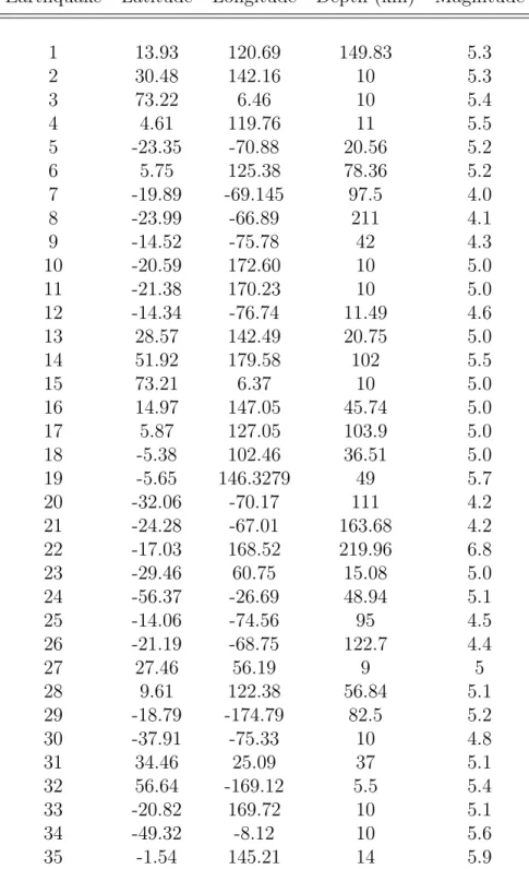
this deployment, 35 teleseismic earthquakes were used to generate 423 receiver functions. From 200

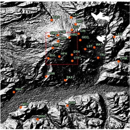
the 25 stations, the stations near the peak of the volcano (denoted by the red box) were primarily 201

focused on. Furthermore, station BAD was not considered due to a suspected error with the seis-202

mometer to earth coupling. 203

In calculating the receiver functions, the iasp91 earth model was used. In the iterative decon-204

volution procedure, a Gaussian width of 5 was also used. Standard errors on the H-κ results were 205

Figure 3: Seismic station deployment around the Llaima Volcano in Chile.The stations focused on in this study are denoted by the red box.

Earthquake Latitude Longitude Depth (km) Magnitude

1 13.93 120.69 149.83 5.3

2 30.48 142.16 10 5.3

3 73.22 6.46 10 5.4

4 4.61 119.76 11 5.5

5 -23.35 -70.88 20.56 5.2

6 5.75 125.38 78.36 5.2

7 -19.89 -69.145 97.5 4.0

8 -23.99 -66.89 211 4.1

9 -14.52 -75.78 42 4.3

10 -20.59 172.60 10 5.0

11 -21.38 170.23 10 5.0

12 -14.34 -76.74 11.49 4.6

13 28.57 142.49 20.75 5.0

14 51.92 179.58 102 5.5

15 73.21 6.37 10 5.0

16 14.97 147.05 45.74 5.0

17 5.87 127.05 103.9 5.0

18 -5.38 102.46 36.51 5.0

19 -5.65 146.3279 49 5.7

20 -32.06 -70.17 111 4.2

21 -24.28 -67.01 163.68 4.2

22 -17.03 168.52 219.96 6.8

23 -29.46 60.75 15.08 5.0

24 -56.37 -26.69 48.94 5.1

25 -14.06 -74.56 95 4.5

26 -21.19 -68.75 122.7 4.4

27 27.46 56.19 9 5

28 9.61 122.38 56.84 5.1

29 -18.79 -174.79 82.5 5.2

30 -37.91 -75.33 10 4.8

31 34.46 25.09 37 5.1

32 56.64 -169.12 5.5 5.4

33 -20.82 169.72 10 5.1

34 -49.32 -8.12 10 5.6

35 -1.54 145.21 14 5.9

Station Latitude Longitude Number of Traces

BAD -38.6441 -71.7829 15

BVL -38.7561 -71.7925 23

CHM -38.7560 -71.5855 13

CIN -38.6844 -71.7029 17

CTF -38.7637 -71.7217 8

DTH -38.7457 -71.7227 11

GEO -38.7029 -71.6982 12

HFH -38.7510 -71.7603 18

HRD -38.6955 -71.7303 7

HRS -38.7259 -71.7800 18

LAG -38.6935 -71.5980 24

LAH -38.6364 -71.7253 23

LST -38.7292 -71.6837 15

MAG -38.8551 -71.8941 12

MDV -38.8996 -71.8741 16

MIC -38.6565 -71.7123 2

PAX -38.8203 -71.7430 18

POW -38.8094 -71.7993 2

RAB -38.8949 -71.7367 8

RLW -38.7059 -71.7639 11

ROD -38.9348 -71.8244 3

SCT -38.6729 -71.7235 17

SMM -38.6908 -71.7914 27

STM -38.6879 -71.7651 21

TRL -38.7545 -71.6456 11

Table 2: The data for the 25 deployed seismic stations

4

Results and Discussion

207

Before this study, the internal plumbing system of Llaima was largely unknown. [Bathke et al., 208

2011] applied inverse modeling to InSAR data and proposed structures at both 4-9 km and 6-12 209

km, however these results are contested. Maisonneuve et al. [2012], using evidence from petrologic 210

data, proposed a magmatic body≤4 km beneath the volcano with an accompanying dike complex. 211

However, these conjectured structures have not previously been confirmed using seismic data. 212

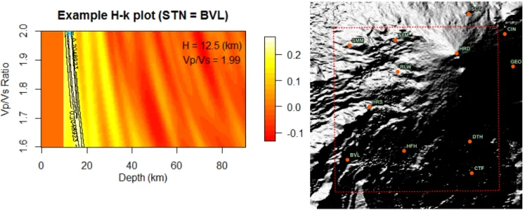
discon-tinuity (H) converged to shallow values for some stations (e.g. station BVL). 214

Figure 5: The initial H-κplot of station BVL.

Figure 6: The red box (Figure 3) inset of the Llaima stations.

As the Moho in the southern Andes is between 30 and 40 km [Tassara et al., 2006], this 215

data suggests that there are other discontinuities under Llaima that could cause P-wave to S-wave 216

conversions. To search for possible converters, slices of depth structure were examined using the 217

H-κ stacking method. 218

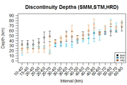
Figure 8: Possible discontinuities revealed by slices of earth structure.

Figure 9: Possible discontinuities revealed by slices of earth structure.

This method of searching in depth intervals could also be interpreted as bandpass filtering 219

the H-κ algorithm results, where the maximum overlap was returned in a depth band. From the 220

resulting search, two main discontinuities are evident, one at approximately 20 km and another at 221

approximately 60 km. While this value is deeper than expected for the region [Tassara et al., 2006], 222

The 20 km discontinuity is interpreted as an area of partial melting beneath Llaima. It is 224

visible on all 9 stations focused on in this study with the exception of station SMM (Figures 7, 8, 225

and 9). 226

From the collection of stations CTF, DTH, and HFH (Figure 7), a possible converter around 227

40 km depth is possible, but more analysis is necessary. In particular, this converter is not visible 228

on the nearby station CTF, so the ray paths to stations DTH and HFH need to be examined. 229

Other possible discontinuities are possible within the region, and one interpretation of the 230

complex converter pattern seen in Figure 8 and Figure 9 is that there is a system of complex 231

melting geometries beneath the volcano. However, it needs to be stressed as well that some of 232

these possible discontinuities may be numerical artifacts stemming from the division of depth into 233

intervals that include neither the 20 km discontinuity or the 60 km discontinuity. 234

5

Conclusions

235

This study presents a first look at the deep magmatic system structure underneath the Llaima 236

volcano in Chile. By applying receiver functions taken from a dense array around the volcano, it was 237

determined that a magmatic body is present at approximately 20 km depth beneath the volcano. 238

This partial melt body could be feeding the shallow region proposed by [Maisonneuve et al., 2012] 239

via the dike system. 240

In future work, forward modeling using synthetic receiver functions [Ammon et al., 1990] can 241

be used to examine these discontinuities further. For an example of this technique, see Chmeilowski 242

et al. [1999]. Furthermore, more analysis can be completed on the Vp/Vs ratios obtained from

243

the H-κ stacks for the region, which provides more information on the percentage of partial melt 244

[Chevrot, 2000]. 245

References

chamber. Geophysical Journal International, na(175):1298–1308, June 2008.

C.J. Ammon, G.E. Randall, and G. Zandt. On the nonuniqueness of receiver function inversions. Journal of Geophysical Research, 95(B10):303–315, September 1990. URL http://onlinelibrary.wiley.com/doi/10.1029/JB095iB10p15303/epdf.

H. Bathke, M. Shirzaei, and T. R. Walter. Inflation and deflation at the steep-sided llaima stratovol-cano (chile) detected by using insar. Geophysical Research Letters, 38(10):n/a–n/a, 2011. ISSN 1944-8007. doi: 10.1029/2011GL047168. URL http://dx.doi.org/10.1029/2011GL047168. L10304.

Maurizio Battaglia, Claudia Troise, Francesco Obrizzo, Folco Pingue, and Giuseppe De Natale. Evidence for fluid migration as the source of deformation at campi flegrei caldera (italy). Geo-physical Research Letters, 33(1):n/a–n/a, 2006. ISSN 1944-8007. doi: 10.1029/2005GL024904. URL http://dx.doi.org/10.1029/2005GL024904. L01307.

Robert D. Chevrot, Sebastien; van der Hilst. The poisson ratio of the australian crust: geological and geophysical implications. Earth and Planetary Science Letters, 183:121–132, August 2000.

J. Chmeilowski, G. Zandt, and C. Haberland. The central andean altiplano-puna magma body. Geophysical Research Letters, 26(6):783–786, March 1999.

Rob W. Clayton and Ralph A. Wiggins. Source shape estimation and deconvolution of teleseismic bodywaves. Geophys. J. R. astr. Soc., 47:151–177, April 1976.

F.A. Darbyshire, K.F. Priestly, R.S. White, R. Stefansson, G.B. Gudmundsson, and S.S. Jakob-sdottir. Crustal structure of central and northern iceland from analysis of teleseismic receiver functions. Geophysical Journal International, na(143):163–184, May 2000.

J. Dawson and P. Tregoning. Uncertainty analysis of earthquake source parameters de-termined from insar: A simulation study. Journal of Geophysical Research: Solid Earth, 112(B9):n/a–n/a, 2007. ISSN 2156-2202. doi: 10.1029/2007JB005209. URL http://dx.doi.org/10.1029/2007JB005209. B09406.

B. Efron. Bootstrap methods: Another look at the jackkife. The Annals of Statistics, 7(1):1–26, 1979.

B. Efron and R. Tibshirani. Boostrap methods for standard errors, confidence intervals, and other measures of statistical accuracy. Statistical Science, 1(1):54–77, 1986.

T. J. Fournier, M. E. Pritchard, and S. N. Riddick. Duration, magnitude, and frequency of sub-aerial volcano deformation events: New results from latin america using insar and a global synthesis. Geochemistry, Geophysics, Geosystems, 11(1):n/a–n/a, 2010. ISSN 1525-2027. doi: 10.1029/2009GC002558. URL http://dx.doi.org/10.1029/2009GC002558. Q01003.

Louis A. Jaeckel. The infintismal jackknife, 1972. URL

J. Julia and J. Mejia. Thickness and vp/vs ratio variation in the iberian crust. Geophysical Journal International, na(156):59–72, September 2004. doi: 10.1111/j.1365-246X.2004.02127.x.

Kikuchi and Kanamori. Inversion of complex body waves. Bulletin of the Seismological Society of America, 72(2):491–506, April 1982.

Charles A. Langston. The effect of planar dipping structure on source and receiver responses for constant ray parameter. Bulletin of the Seismological Society of America, 67(4):1029–1050, August 1977b.

Charles A. Langston. Structure under mount ranier, washington, inferred from teleseismic body waves. Journal of Geophysical Research, 84(B9):4749–4762, August 1979.

Z. Li. Meris atmospheric water vapor correction model for wide swath interferometric synthetic aperture radar. IEEE Geoscience and Remote Sensing Letters, 9(2):257–261, October 2011.

Ligorra and Ammon. Iterative deconvolution and receiver-function estimation. Bulletin of the Seismological Society of America, 89(5):1395–1400, October 1999.

D. Lombardi, J. Braunmiller, E. Kissling, , and D. Giardini. Moho depth and poisson’s ratio in the western-central alps from receiver functions. Geophysical Journal International, na(173):249–264, November 2008.

Zhong Lu and Daniel Dzurisin. InSAR Imaging of Aleutian Volcanoes, volume 1. Springer Berlin Heidelberg, 2014.

C.B. Maisonneuve, M.A. Dungan, O. Bachmann, and A. Burgisser. Insights into shallow magma storage and crystallization at volcn llaima (andean southern volcanic zone, chile). Journal of Vol-canology and Geothermal Research, 211-212:76–91, 2012. doi: 10.1016/j.jvolgeores.2011.09.010.

Rupert G. Miller. The jackknife - a review. Biometrika, 61(1):1–15, April 1974. URL http://www.jstor.org/stable/2334280.

H. Nakamichi, Tanaka S., and Hamaguchi H. Fine s wave velocity structure beneath iwate volcano, northeastern japan, as derived from receiver functions and travel times. Journal of Volcanology and Geothermal Research, 116(na):235–255, July 2001.

J.A. Naranjo and H. Moreno. Geologa del volcn Llaima . SERNAGEOMIN, Chile. Carta Geolgica de Chile, No.88, mapa escala 1:50.000. Number 88 in n/a. Gobierno de Chile Servicio Nacional de Geologia y Mineria, Santiago, Chile, 2005.

Jose A. Naranjo and Hugo Moreno. Actividad explosiva postglacial en el volcan llaima, andes del sur (3845?s). Revista Geolgica de Chile, 18(1):69–80, na 1991.

D. W. Oldenburg. A comprehensive solution to the linear deconvolution problem. Geophys. J. R. astr. Soc., 65:331–357, April 1981.

Jeffrey Park and Vadim Levin. Receiver functions from multiple-taper spectral correlation estimates. Bulletin of the Seismological Society of America, 90(6):1507–1520, December 2000.

D. Remy, Y. Chen, J. L. Froger, S. Bonvalot, L. Cordoba, and J. Fustos. Revised inter-pretation of recent insar signals observed at llaima volcano (chile). Geophysical Research Letters, 42(10):3870–3879, 2015. ISSN 1944-8007. doi: 10.1002/2015GL063872. URL http://dx.doi.org/10.1002/2015GL063872. 2015GL063872.

A. Tassara, H.J. Gotze, S. Schmidt, and R. Hackney. Three-dimensional density model of the nazca plate and the andean continental margin.Journal of Geophysical Research, 111(B09404):na, 2006. doi: 10.1029/2005JB003976, 200.

Tohru Watanabe. Effects of water and melt on seismic velocities and their application to charac-terization of seismic reflectors. Geophysical Research Letters, 20(24):2933–2936, December 1993.