ENVIRONMENTAL LIMITATIONS TO FOREST GROWTH AND PRODUCTIVITY IN NORTH AMERICA
Matthew P. Dannenberg
“A dissertation submitted to the faculty at the University of North Carolina at Chapel Hill in partial fulfillment of the requirements for the degree of Doctor of Philosophy in the
Curriculum of Geography.”
Chapel Hill 2017
Approved by: Conghe Song Erika Wise Aaron Moody
©2017
ABSTRACT
Matthew P. Dannenberg: Environmental Limitations to Forest Growth and Productivity in North America
(Under the direction of Conghe Song and Erika Wise)
Terrestrial primary production—the carbohydrates produced by plants via
photosynthesis—is the entry point of energy and carbon into ecosystems, forming the base of the food chain and a sink for anthropogenic CO2. Primary production can be limited by unfavorable environmental conditions, including non-optimal temperatures, water deficits, or inadequate nutrient supply. At present, our ability to model how environmental factors reduce primary production remains limited. This leads to uncertainty both in the remotely sensed models used to monitor primary production and in climate models that depend on accurate representation of the land surface and biosphere.
Given the importance of vegetation to humanity and the Earth system, in this
dissertation I use tree rings and remote sensing to examine the environmental drivers of forest growth and productivity in North America. In particular, this research examines how forests are influenced by climate, atmospheric circulation, and land surface characteristics like topography and soil quality. I first examine how the seasonality of temperature and
ACKNOWLEDGEMENTS
Many individuals have contributed to the research presented in this dissertation. First and foremost, I thank my graduate advisors, Conghe Song and Erika Wise, for their many years of support, mentorship, and guidance. This work would not have been possible without them. I also thank the members of my graduate committee—Aaron Moody, Tamlin Pavelsky, and Diego Riveros-Iregui—for their comments and feedback over the years, which were instrumental in improving this research. Thank you as well to the anonymous reviewers whose comments on my manuscripts have contributed to the improvement of this dissertation. I am also grateful for the support of other graduate students in the Song and Wise labs, particularly Chris Hakkenberg and Qi Zhang. Finally, this research was supported by a small army of undergraduate and graduate research assistants (Kelsey Ajo, Dusty Grossheim, Chris Jones, Jocelyn Keung, Holly Kuestner, Claire Nelson, Zachary Pope, Melissa Wrzesien, and Lillian Wu), each of whom contributed in various ways to the collection and processing of datasets that were used in this dissertation.
This work was funded in part by NSF Paleo Perspectives on Climate Change (P2C2) grants 1102757 and 1304422, as well as by a Dissertation Completion Fellowship and the Ed and Carol Smithwick Summer Research Fellowship (both from UNC-Chapel Hill) and a Dissertation Research Grant from the American Association of Geographers. Many of the datasets used in this research were freely provided by the International Tree-Ring Data Bank, the Global Inventory Modeling and Mapping Studies (GIMMS), the USDA Natural
TABLE OF CONTENTS
LIST OF TABLES... x
LIST OF FIGURES ... xi
LIST OF ABBREVIATIONS ... xiv
CHAPTER 1: INTRODUCTION ... 1
Overview ... 1
Background ... 4
Environmental limitations to vegetation activity ... 4
The canopy and the cambium: two perspectives on vegetation activity ... 6
Dissertation Structure and Contributions ... 8
Summary of Chapter 2 ... 9
Summary of Chapter 3 ... 10
Summary of Chapter 4 ... 11
Overall contributions of the dissertation... 12
CHAPTER 2: SEASONAL CLIMATE SIGNALS FROM MULTIPLE TREE-RING METRICS: A CASE STUDY OF PINUS PONDEROSA IN THE UPPER COLUMBIA RIVER BASIN... 13
Introduction ... 13
Data and Methods ... 16
Study Area and Climate Data ... 16
Tree-Ring Data ... 17
Analyses ... 18
Results ... 22
Discussion ... 28
CHAPTER 3: ENVIRONMENTAL STRESSES TO PRIMARY PRODUCTION IN THE
CONTERMINOUS UNITED STATES... 34
Introduction ... 34
Data and Methods ... 37
A Tree-Ring Based Environmental Stress Index ... 37
Tree-Ring Data ... 39
Evaluation of Tree-Ring Environmental Stress Estimates ... 41
Climate, topography and soil data... 43
Modeling the Environmental Drivers of Stress ... 44
Results ... 47
Evaluation of the Tree-Ring Environmental Stress Index ... 47
Environmental Drivers of Stress ... 49
Discussion ... 54
CHAPTER 4: SHIFTING PACIFIC STORM TRACKS AS STRESSORS TO ECOSYSTEMS OF WESTERN NORTH AMERICA ... 58
Introduction ... 58
Materials and Methods ... 60
Estimation of the historical Pacific storm track ... 60
Hydrological variables and analyses ... 61
Ecological variables and analyses ... 62
Results ... 67
Historical variation of cool-season Pacific storm tracks ... 67
Hydrological responses to shifting Pacific storm tracks... 68
Ecosystem responses to shifting Pacific storm tracks ... 71
Discussion ... 76
CHAPTER 5: SUMMARY AND CONCLUSIONS ... 78
APPENDIX 1: SUPPLEMENTAL FIGURES ... 82
LIST OF TABLES
Table 1.1. Complementary characteristics of remote sensing and tree-ring
estimates of vegetation activity ... 8 Table 2.1. Effective correlations between Pcool and tree-ring PCs, and the
variance-scaled R2 (R2
vs) and extreme value capture statistics for both extreme low (EVClow) and extreme high precipitation (EVChigh) events
for COMBO composites ... 21 Table 2.2. Effective correlations between Pwarm and tree-ring PCs, and the
variance-scaled R2 (R2
vs) and extreme value capture statistics for both extreme low (EVClow) and extreme high precipitation (EVChigh) events
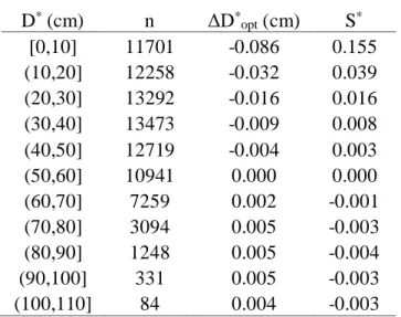
for COMBO composites ... 22 Table 2.3. Shared variance (r2) among PC1 metrics and among PC2 metrics ... 23 Table 3.1. Structure of the random forest model experiments ... 46 Table 3.2. Median bias in ΔD*
opt and S* for different diameter classes ... 48 Table A1. Summary of tree-ring chronologies over the period 1913-2012 ... 108 Table A2. Mean inter-series correlations between trees (RBARbt), within
trees (RBARwt), and total (RBARtot); effective mean inter-series correlations (RBAReff); signal-to-noise ratio (SNR); and expressed population signal (EPS) for CooRecorder parameter sets over the
period 1913-2012 ... 109 Table A3. Percent variance explained by PC1 and PC2 of each tree-ring metric ... 111 Table A4. Species present in ITRDB sites used in this study (with the number,
n, of sites for each species), and parameters used in the optimal growth model: growth rate factor (G), maximum diameter (Dmax, in cm),
maximum height (Hmax, in cm), and maximum age (AGEmax) ... 112 Table A5. Model statistics for the full TSC ecoregion RF models of absolute
stress (based on out-of-bag observations), and change in variance
explained (Δr2) when using a partial model ... 113 Table A6. Model statistics for the full TSC ecoregion RF models of relative
stress (based on out-of-bag observations), and change in variance
LIST OF FIGURES
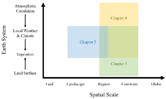
Figure 1.1. The Earth system perspective on the environmental limitations to
vegetation activity that underlies this dissertation ... 3
Figure 1.2. Spatial scales and Earth systems examined in each chapter ... 9
Figure 2.1. Six tree-ring sites in and surrounding the upper Columbia River Basin... 17
Figure 2.2. Pearson correlation coefficients between the first principal component of each tree-ring metric and 3-month precipitation composites ... 24
Figure 2.3. Pearson correlation coefficients between the second principal component of each tree-ring metric and 3-month precipitation composites ... 26
Figure 2.4. Time plots and scatter plots of observed and predicted October- March precipitation (Pcool) and May-August precipitation (Pwarm) in the CRB based on CPS models ... 27
Figure 3.1. Level I ecoregions and distribution of tree-ring sites and flux towers ... 40
Figure 3.2. Flow chart of ecoregion-level environmental stress models... 45
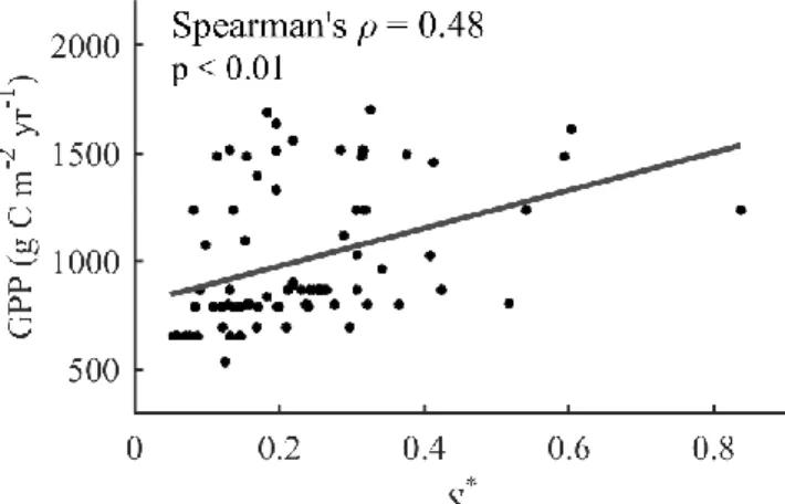
Figure 3.3. Relationship between annual 𝑆∗ and annual GPP at flux towers within 100 km of tree-ring sites ... 49
Figure 3.4. Spearman’s rank correlation coefficient (ρ) between 𝑆∗ and seasonal minimum (TMIN) and maximum (TMAX) temperatures... 50
Figure 3.5. Spearman’s rank correlation coefficient (ρ) between 𝑆∗ and seasonal vapor pressure deficit (VPD) and water balance (WB) ... 52
Figure 3.6. Random forest model strength (r2) for explaining variation in environmental stress ... 53
Figure 4.1. Delineation of the cool-season storm track in an example year (1988) ... 61
Figure 4.2. Raw and smoothed NDVI time series for six example ecoregions ... 64
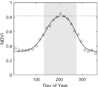
Figure 4.3. Calculation of land surface phenology metrics ... 65
Figure 4.4. Storm track trajectories from 1980-2014 ... 68
Figure 4.5. Relationship between Pacific storm track position and drought and snowpack ... 69
Figure 4.6. Relationship between Pacific storm track position and NDVImax ... 72
Figure 4.8. Relationship between Pacific storm track position and fire area... 75 Figure A1. Mean monthly temperature and precipitation for the period 1981-
2010 in the upper CRB ... 82
Figure A2. Biplot of factor loadings for the first two principal components for
each metric ... 83 Figure A3. Relationship between mean elevation of trees included in each site
chronology and PC2 loadings ... 84 Figure A4. Scree plot of PC eigenvalues for each tree-ring metric ... 85 Figure A5. Seasonal correlations between precipitation and maximum
temperature and PC1 of residual chronologies of (a) TRW, (b) EW,
(c) LWadj, and (d) BI ... 86 Figure A6. Seasonal correlations between precipitation and maximum
temperature and PC2 of residual chronologies of (a) TRW, (b) EW,
(c) LWadj, and (d) BI ... 87 Figure A7. Seasonal correlations between precipitation and maximum
temperature and PC1 of standard chronologies of (a) TRW, (b) EW,
(c) LWadj, and (d) BI ... 88 Figure A8. Seasonal correlations between precipitation and maximum
temperature and PC2 of standard chronologies of (a) TRW, (b) EW,
(c) LWadj, and (d) BI ... 89 Figure A9. Six ponderosa pine tree-ring sites in the Pacific Northwest, where
in situ DBH measurements are available ... 90 Figure A10. Potential outcomes from increment cores ... 91 Figure A11. Number of tree-ring sites and site-years within each ecoregion... 92 Figure A12. Comparison of in situ measured DBH to ring-width-based
estimates of DBH for 276 increment cores from six sites in the Pacific
Northwest ... 93 Figure A13. Bias in ∆𝐷𝑜𝑝𝑡∗ (relative to ∆𝐷𝑜𝑝𝑡) for 10 cm diameter classes at
six ponderosa pine sites in the Pacific Northwest ... 94 Figure A14. Bias in 𝑆∗ (relative to 𝑆) for 10 cm diameter classes at six
ponderosa pine sites in the Pacific Northwest ... 95 Figure A15. Spearman’s rank correlation coefficient (ρ) between 𝑆𝑟 and
Figure A16. Spearman’s rank correlation coefficient (ρ) between 𝑆𝑟 and
seasonal vapor pressure deficit (VPD) and water balance (WB) ... 97 Figure A17. Relationship between Pacific storm track position and precipitation ... 98 Figure A18. Relationship between monthly Pacific storm track position and drought.... 99 Figure A19. Relationship between monthly Pacific storm track position and
snowpack ... 100 Figure A20. Relationship between Pacific storm track position and streamflow ... 101 Figure A21. Relationship between Pacific storm track intensity and drought and
snowpack ... 102 Figure A22. Relationship between Pacific storm track position and start of green
season ... 103 Figure A23. Relationship between Pacific storm track position and end of green
season ... 104 Figure A24. Relationship between Pacific storm track position and length of green
LIST OF ABBREVIATIONS AVHRR Advance Very High Resolution Radiometer BI Blue intensity
CPS Composite-plus-scale CRB Columbia River basin DBH Diameter at Breast Height EPS Expressed Population Signal EVC Extreme value capture
EW Earlywood width
GPP Gross Primary Production
ITRDB International Tree-Ring Data Bank LUE Light-Use Efficiency
LW Latewood width
LWadj Adjusted latewood width
NDVI Normalized difference vegetation index PAR Photosynthetically active radiation PCA Principle component analysis Pcool Cool-season precipitation Pwarm Warm-season precipitation
RF Random Forest
SPEI Standardized Precipitation-Evapotranspiration Index SWE Snow water equivalent
TWI Topographic Wetness Index UAA Upslope Accumulated Area VPD Vapor Pressure Deficit
CHAPTER 1: INTRODUCTION
Overview
Vegetation on Earth’s land surface provides many of the key resources and services that humans and other animals rely upon. Terrestrial primary production—the carbohydrates produced by plants via photosynthesis—is the entry point of energy and carbon into
ecosystems and the fundamental source of food for all land-dwelling organisms [Chapin et al., 2011]. Recent estimates suggest that approximately 80% of available net primary production has already been appropriated for human use, with the remainder representing a key “planetary boundary” for future human activity [Running, 2012]. Uptake of CO2 through plant productivity is also a major component of the global carbon cycle [Pan et al., 2011]. Historically, primary production by terrestrial vegetation has acted as a large sink for CO2, with approximately 25% of annual anthropogenic CO2 emissions being removed from the atmosphere by plants [Ciais et al., 2013].
The productivity of terrestrial vegetation can be limited or co-limited by multiple climate or environmental factors [Nemani et al., 2003; Garbulsky et al., 2010]. Precise
knowledge of the environmental drivers of vegetation productivity is therefore needed both to monitor current vegetation activity over large areas and to project potential changes in
ecosystem structure and function under a changing climate. At present, this knowledge is limited, particularly regarding how environmental limitations to plant growth vary spatially and temporally over large areas. The current generation of remotely sensed primary
production models, for example, generally assume instantaneous responses of plant
the effects of soils, topography, and lags between the climate system and plant activity. Estimating the effects of water stress on primary production is particularly challenging [Zhang et al., 2015], and error in primary production estimates derived from remotely sensed data can partly be traced to uncertainties in the parameterization of these environmental limitations [Cai et al., 2014]. Likewise, global climate models depend on accurate representation of environmental limitations to vegetation productivity. While projected changes in temperature, hydroclimate, and atmospheric circulation during the 21st century will likely have a strong impact on the primary production of the biosphere, there remains significant disagreement over whether the positive influences of climate change on vegetation (e.g., CO2 fertilization and longer growing seasons) will outweigh its negative consequences (e.g., greater water stress and higher respiration rates) [Settele et al., 2014; Allen et al., 2015; Smith et al., 2016; Ballantyne et al., 2017].
Given the importance of vegetation for provisioning of ecosystem goods and services to humanity, as well as the current limitations in our understanding of how vegetation is limited by environmental conditions, my research is motivated by a fundamental question of contemporary biogeoscience: how do vegetated ecosystems interact with and respond to variation in other Earth systems? In this dissertation, I examine the environmental drivers of vegetation activity in North America and how sensitivity to those environmental drivers varies spatially and temporally. In particular, this work focuses on how vegetation activity in North America is influenced by three interacting components of the atmosphere and
lithosphere (Figure 1.1):
(2) Atmospheric circulation systems, particularly midlatitude storm tracks, which are largely responsible for water delivery to western North America.
(3) Land surface characteristics, specifically topography and soil structure and quality, that affect the ability of plants to obtain belowground resources like soil water and nutrients.
Figure 1.1. The Earth system perspective on the environmental limitations to vegetation activity that underlies this dissertation. The general Earth system of interest is represented in bold and underlined text, while the specific processes examined are represented in smaller text below each system.
In this Introduction, I first review the necessary background for the dissertation, focusing on two aspects of previous work that are relevant to all subsequent chapters: (1) the current state of knowledge regarding climatic and land surface limitations to vegetation activity, particularly at the level of individual plants, and (2) the two different, but
and findings of each individual chapter. I conclude with a summary of how this dissertation will contribute to current conversations in the fields of physical geography and
biogeoscience.
Background
Environmental limitations to vegetation activity
In order to assess the environmental drivers of vegetation activity over a large area, which is the fundamental goal of my dissertation, it is necessary to understand the
physiological processes that connect individual plants with their environment. At the leaf level, the photosynthetic process starts with diffusion of CO2 from the atmosphere into leaves through the stoma. However, when stomata are open, water is also lost from the leaf to the atmosphere. This loss of water from the leaf is replenished by water from the soil. To prevent excessive loss of water, plants regulate stomatal apertures based on the availability of soil moisture and the strength of the atmospheric sink for moisture. Low soil moisture, high vapor pressure deficit, and low leaf water potential therefore limit photosynthesis by restricting diffusion of CO2 into stomata.
Moisture stress can also directly affect photosynthetic processes through metabolic damage or down-regulation (e.g., reduced ATP and RuBP synthesis or permanent
reducing the capacity of plants to repair damage, and by exacerbating temperature-induced damage to the photosynthetic apparatus [Allakhverdiev et al., 2008].
Temperature can affect vegetation activity both directly and indirectly. For example, temperature directly affects the rates of biochemical reactions in photosynthesis, with optimal temperatures that vary among different plant species and biomes [Pallardy, 2008]. At low temperatures, biochemical reactions occur at slower rates while high temperatures can lead to enzyme deactivation, protein denaturation, damage to photosystem II, generation of reactive oxygen species, and increased photorespiration [Allakhverdiev et al., 2008; Pallardy, 2008]. Freezing temperatures also subject plants to increased risk of xylem embolisms and cavitation [Pallardy, 2008; Chapin et al., 2011] and limit the ability of plant roots to obtain
belowground resources [Archibold, 1995]. Temperature is a dominant control on the length of the vegetation growing season [Richardson et al., 2013], though changes in the length of the growing season do not necessarily lead to proportional increases in primary production or net ecosystem exchange due to the effects of temperature on water availability and ecosystem respiration [Angert et al., 2005; Hu et al., 2010; Brzostek et al., 2014; Zhang et al., 2014; Dannenberg et al., 2015]. In arid and semi-arid regions, high temperatures can exacerbate soil water limitation through increases in vapor pressure deficit and evaporative demand, which can lead to stomatal closure and thus lower rates of carbon assimilation [McDowell et al., 2011; Williams et al., 2013].
Finally, non-climatic environmental factors, such as soils and topography, can affect primary production through their control on the ability of plants to obtain necessary
Chapin et al., 2011]. Structural characteristics of soils, including soil depth and porosity, affect soil water storage and the ease with which plants can extract water from the soil [Chapin et al., 2011; Hornberger et al., 2014]. Likewise, topography affects the lateral redistribution of water within a watershed [Beven and Kirkby, 1979; Hornberger et al., 2014], which is an important control on soil moisture [Western et al., 1999] and therefore on ecosystem carbon and water fluxes [Riveros-Iregui and McGlynn, 2009; Emanuel et al., 2010, 2011; Riveros-Iregui et al., 2011]. Land surface characteristics like topography and soil structure and quality therefore represent important spatial constraints on the ability of plants to obtain belowground resources like water and nutrients.
The canopy and the cambium: two perspectives on vegetation activity
Variation in climate and land surface characteristics can affect vegetation processes both in the leaves of plant canopies and in the vascular cambium, which can be measured using remote sensing and tree rings, respectively. At the canopy level, solar radiation in the visible spectrum (i.e., photosynthetically active radiation (PAR)) provides the energy to drive photosynthesis. Healthy, productive plant canopies therefore tend to absorb most incoming PAR, while reflecting or transmitting most incoming near infrared radiation. The reflectance of the land surface in these spectral regions can be estimated through remote sensing,
primary production [e.g., Running et al., 2004], and land surface phenology [e.g., Moody and Johnson, 2001].
The carbohydrates produced through photosynthesis provide both the energy and the molecular structure needed for cell division and expansion in the vascular cambium of woody tissues [Fritts, 1976; Pallardy, 2008]. In regions where photosynthetic and cambial processes are limited by climate (either temperature or water availability), the widths of tree rings may vary annually as a function of climate. This variability provides the fundamental basis for using tree rings as proxies for past variation in temperature [e.g., Mann et al., 1998, 2008; Luterbacher et al., 2004], precipitation [e.g., Neukom et al., 2010; Yi et al., 2012], streamflow [e.g., Wise, 2010c; Littell et al., 2016], and atmospheric circulation [e.g., Wise and
Dannenberg, 2014]. The annual tree rings formed through cambial processes also represent the primary production that is allocated to woody growth, allowing long-term estimates of annual aboveground primary production based on measurements of tree-ring widths [e.g., Graumlich et al., 1989; Rathgeber et al., 2000]. Unlike remote sensing, tree-ring
chronologies are located at discrete point locations and do not provide continuous spatial coverage of vegetation processes. However, they have demonstrated significant skill at representing productivity across entire landscapes [Beck et al., 2013; Bunn et al., 2013], including for grasslands near the tree-ring site [Liang et al., 2009], suggesting that tree rings are likely useful indicators of ecosystem productivity across large regions and even for regions dominated by other plant functional types.
perspectives on the terrestrial carbon cycle across a range of spatial, temporal, and process scales [Babst et al., 2014].
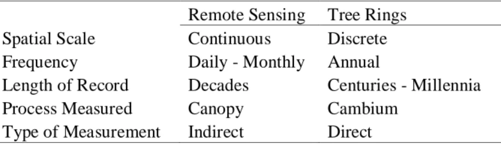
Table 1.1. Complementary characteristics of remote sensing and tree-ring estimates of vegetation activity.
Remote Sensing Tree Rings Spatial Scale Continuous Discrete Frequency Daily - Monthly Annual
Length of Record Decades Centuries - Millennia
Process Measured Canopy Cambium
Type of Measurement Indirect Direct
Dissertation Structure and Contributions
Figure 1.1. Spatial scales and Earth systems examined in each chapter.
Summary of Chapter 2
Research Questions: How does sub-annual growth of a prominent tree species in the western U.S. (Pinus ponderosa subsp. ponderosa) respond to seasonal climate variability? What are the implications of that response both for reconstruction of past climate and for understanding the consequences of future hydroclimatic change for these ecosystems?
Aims and Methods: In this chapter, I examine how the seasonality of precipitation and temperature affect tree growth, as measured by total ring width, earlywood width, adjusted latewood width, and blue intensity chronologies from a network of six Pinus ponderosa sites in and surrounding the upper Columbia River basin of the U.S. Pacific Northwest. I also evaluate the potential for combining multiple tree-ring metrics together in reconstructions of past cool- and warm-season precipitation.
elevation sites also show relatively strong dependence on cool-season moisture. Temperature is not strongly limiting at any of the sites nor for any tree-ring metric. Effective correlation analyses and composite-plus-scale tests suggest that combining multiple tree-ring metrics together may improve reconstructions of warm-season precipitation. For cool-season precipitation, total ring width alone explains more variance than any other individual metric or combination of metrics. The composite-plus-scale tests show that ponderosa pine tree rings in the upper Columbia River basin are asymmetric in their responses precipitation extremes: while growth indices strongly reflect low (but not high) precipitation extremes during the cool season, they reflect high (but not low) precipitation extremes during the warm season.
Summary of Chapter 3
Research Questions: What are the dominant sources of “environmental stress” in vegetated ecosystems of the conterminous United States? How responsive are these
ecosystems to climate conditions prior to the growing season? What are the consequences of failing to account for topography and soil characteristics in models of environmental stress? Aims and Methods: I develop a data-driven approach for estimation of environmental stress effects on forest growth (based on tree-ring widths) and assess the environmental drivers of both spatial and temporal variation of forest growth stress. I first test and evaluate the new environmental stress index at six ponderosa pine tree-ring sites in the U.S. Pacific Northwest and then apply the index to a large network of tree-ring widths across the conterminous United States. Finally, I use correlation analyses and a series of machine learning model experiments to examine the climatic, topographic, and edaphic drivers of growth in ecoregions of the U.S.
the environmental stress index captures meaningful information on primary production at the continental scale. Tree growth in ecosystems of the western United States relies on water that is delivered prior to the growing season, a key finding given that many primary production models do not include physically-meaningful lags between the climate system and ecosystem carbon uptake. In addition, topographic and soil characteristics, which are not typically included in the current generation of remote sensing-based primary production models, are important drivers of spatial gradients in mean environmental stress in most of the eastern U.S.
Summary of Chapter 4
Research Questions: How have the hydroclimate and water resources of western North America responded to historical Pacific storm track variability? How have storm track-induced changes in water supply affected primary production, phenology, and fire regimes in this region?
Aims and Methods: I estimate cool-season Pacific storm track position and intensity for the period 1980-2014 using 300 hPa meridional wind velocity from the North American Regional Reanalysis. Using historical climate data, I examine the sensitivity of water
resources (the climatic water balance, snowpack, and streamflow) to variation in the position and intensity of the storm track. To examine the sensitivity of ecological systems to storm track variability, I develop or obtain estimates of forest growth, land surface phenology, and wildfire area from a large network of tree-ring widths and remotely sensed data from
AVHRR and Landsat.
Canada but negative correlations in the northwestern U.S. Likewise, tree-ring widths and remotely sensed estimates of peak greenness show that ecosystems of the western U.S. tend to be greener and more productive following winters with south-shifted storm tracks, while Canadian ecosystems tend to be greener in years when the cool-season storm track is shifted to the north. On average, larger areas of the northwestern U.S. are burned by moderate to high severity wildfires when storm tracks are displaced north, and the average burn area per fire also tends to be higher in years with north-shifted storm tracks. A persistent shift in the position of Pacific storm tracks during the 21st century would likely alter hydroclimatic and ecological regimes in western North America, particularly in the western U.S., where water supply and vegetation activity are closely linked to the position of the Pacific storm track.
Overall contributions of the dissertation
CHAPTER 2: SEASONAL CLIMATE SIGNALS FROM MULTIPLE TREE-RING METRICS: A CASE STUDY OF PINUS PONDEROSA IN THE UPPER COLUMBIA
RIVER BASIN1
Introduction
Temperature increases over the 21st century will alter hydroclimatic regimes in many regions, and these impacts will be highly seasonal [Lute et al., 2015]. In the U.S. Pacific Northwest, climate models project relatively little change in total annual precipitation, but this precipitation may be redistributed from the warm season to the cool season, resulting in an enhanced seasonal precipitation cycle in which dry summers become drier and wet winters become wetter [Mote and Salathé, 2010]. Even with projected increases in winter
precipitation, warmer temperatures could lead to reductions in snowpack and an increasingly rain-dominated climate. In the western U.S., for example, climate change has led to
significant reductions in mountain snowpack which are nearly unprecedented in historical and paleoclimate records [Barnett et al., 2005; Mote et al., 2005; Pederson et al., 2011; Luce et al., 2013]. Declining snowpacks, combined with seasonality shifts, are a major challenge for water resource managers in these regions [Hamlet and Lettenmaier, 1999; Leung et al., 2004; Crawford et al., 2015], increasing the need to understand historical variation of
precipitation and drought on sub-annual time scales. These changes in hydroclimate will also have significant consequences for the functioning of terrestrial ecosystems [Settele et al., 2014], including likely changes in vegetation distribution, fire regimes, and carbon uptake
1 This chapter previously appeared as an article in the Journal of Geophysical Research: Biogeosciences. The original citation is as follows:
and storage [Boisvenue and Running, 2010; Rogers et al., 2011; Notaro et al., 2012; Jiang et al., 2013].
The annual growth rings of trees can be used both to understand the sensitivity of tree growth to climate variability and to make inferences about past climate variability and
change, including past variation of hydroclimate on seasonal timescales. Tree rings are frequently used as indicators of past environmental variation due to the sensitivity of cambial processes to climate, the longevity of many tree species, the relative simplicity and cost effectiveness of data collection, and the precise annual crossdating of each ring [Fritts, 1976; Jones et al., 2009; St. George, 2014]. Tree-ring widths and densities have been used to infer past temperatures [Mann et al., 1998, 2008; Jones et al., 2009], precipitation [Touchan et al., 2005; Neukom et al., 2010], atmospheric circulation [Wise and Dannenberg, 2014],
streamflow [Wise, 2010c], snow cover [Pederson et al., 2011], and drought [Cook et al., 1999, 2004]. The climate signals and seasonality recorded in tree rings reflect the
environmental factors that are most limiting to growth, which in turn depend upon both the local environmental conditions, such as climate regime and topography, and the physiology of the tree species, including leaf phenology and longevity [Fritts, 1976]. The climate sensitivity of tree rings therefore varies geographically. In the southwestern U.S., for example, tree growth is most responsive to winter precipitation, while sites at high northern latitudes are often most responsive to temperature [St. George, 2014; St. George and Ault, 2014].
LW reflects warm-season precipitation [Meko and Baisan, 2001; Stahle et al., 2009; Griffin et al., 2013]. Previous studies in western Canada and the U.S. Intermountain West have also examined seasonal climate signals in sub-annual ring widths, including at ponderosa pine and Douglas-fir sites in British Columbia, Canada [Watson and Luckman, 2002] and Douglas-fir sites in Idaho and Montana [Crawford et al., 2015]. Watson and Luckman [2002] found that both EW and LW are positively correlated with summer precipitation, though EW is more sensitive than LW to precipitation in winter and in the year prior to growth. While there is substantial overlap in the seasonal precipitation signals embedded in EW and LW
chronologies, Crawford et al. [2015] found that EW is most sensitive to spring precipitation (April–June) while LW is most sensitive to precipitation later in the growing season (June– August). Neither EW nor LW were strongly correlated with temperature in these studies [Watson and Luckman, 2002; Crawford et al., 2015].
The maximum density of tree-ring latewood is often strongly and positively
dependent on summer temperature [e.g., Briffa et al., 2004; Kirdyanov et al., 2008; Wilson et al., 2014], but it is expensive and time-consuming to obtain. Since the amount of blue light reflected from tree-ring latewood is inversely related to the density of latewood cells, the intensity of blue light reflectance from tree-ring latewood (blue intensity, or BI) can provide a reliable proxy for maximum latewood density with a similar climate signal at a fraction of the cost [McCarroll et al., 2002, 2011; Rydval et al., 2014; Wilson et al., 2014]. Combining multiple tree ring metrics with complementary seasonal climate signals may improve the reconstruction of past climate [McCarroll et al., 2003, 2011].
metrics to seasonal climate variability within the upper CRB and to evaluate the potential for a multi-metric tree ring reconstruction of past precipitation in both the cool and warm
seasons. This work provides additional tests of the climate signals embedded in a relatively new paleoclimate proxy, BI. Results from this study demonstrate the utility of sub-annual ring widths for capturing seasonal climate signals and the potential for combining multiple tree-ring metrics in reconstructions of past hydroclimate on a sub-annual temporal scale in the Pacific Northwest region of the U.S.
Data and Methods
Study Area and Climate Data
Figure 2.1. Six tree-ring sites in and surrounding the upper Columbia River Basin (HUC Subregion 1702; dark grey shading).
Tree-Ring Data
Increment cores were collected from six sites in and surrounding the upper CRB during summers 2011-2014 (Figure 2.1; Table A1). Site elevations ranged from
approximately 825 meters to nearly 1400 meters above sea level. Trees with fire or lightening
al., 2015], an adjusted LW index (LWadj) was developed for each measured core prior to site-level averaging based on the residuals of a linear regression of the detrended LW width on the detrended EW width [Griffin et al., 2011]. After quality control of ring width
measurements using COFECHA [Holmes, 1983] and removing series with low correlations to the master chronologies, most ring-width chronologies achieved an expressed population signal (EPS) > 0.85 over the period 1913-2012 with the exception of LWadj chronologies at sites 1, 2, and 4, which each had EPS > 0.8 (Table A1).
A subset of cores from each site were scanned at 3200 DPI on a flatbed scanner, and BI chronologies were developed using the CooRecorder software [Rydval et al., 2014]. Previous studies have suggested extracting resins from cores prior to scanning using soxhlet extraction or acetone baths [Campbell et al., 2007, 2011; Rydval et al., 2014; Wilson et al., 2014], but I was not able to perform any resin extraction since these cores were subsequently used in isotope analyses. While the lack of resin extraction would likely pose a significant problem for a reconstruction due to large color differences between heartwood and sapwood, I focused solely on the climate signal in tree-ring metrics during the instrumental period (1913-2012). Most BI series consisted entirely of sapwood during the study period, but heartwood–sapwood boundaries were visually identified in the core scans and the heartwood BI was not considered in further analyses. Additional details of the blue intensity
methodology are available in Appendix 3 (Text A1).
Analyses
I examined the sensitivity of different tree-ring metrics to seasonal climate variability using un-rotated principal component analysis (PCA), which I performed separately for each of the four tree-ring metrics over the period 1913-2012 using the six different site
performed using singular value decomposition on the covariance matrices of P. ponderosa
metrics. Using the Seascorr program in the MATLAB programming environment [Meko et al., 2011], I performed running correlations between the first two components of each tree-ring metric (a total of eight chronologies) and 1-, 3-, 6-, and 9-month composites of upper CRB-averaged precipitation (the primary variable) and maximum temperature (the secondary variable). Seasonal correlations between tree-ring metric PCs and the primary variable were calculated using the Pearson correlation coefficient. The relationship between tree-ring metrics and the secondary variable was assessed using partial correlation analysis (i.e., the correlation after the influence of the primary variable is removed), with significance of correlations estimated using Monte Carlo simulations [Meko et al., 2011].
I assessed the potential for combining multiple tree-ring metrics in precipitation reconstructions using composites of the ponderosa pine BI and ring width PCs. Many approaches have been developed for compositing proxy time-series, but compositing
generally involves either a weighted or unweighted averaging of standardized proxy records [Jones et al., 2009]. Here, I standardized the first two PCs of each tree-ring metric to a common mean and variance so that all variables are on the same scale. I then formed a total of 21 composites using weighted averages of different metrics and PCs (Tables 2.1 and 2.2), where the weight was derived from the percentage of the variance explained in a linear relationship between a given component and the climate time-series of interest [McCarroll et al., 2011]. I calculated “effective correlations” [McCarroll et al., 2003, 2011] between these ponderosa pine composites and two precipitation composites: cool-season precipitation (Pcool, defined as the total precipitation from October through March) and warm-season
In addition to the effective correlation analysis, I assessed the potential for a multi-metric tree ring reconstruction of cool- and warm-season precipitation in the upper CRB using a series of composite-plus-scale (CPS) tests. The CPS approach is a flexible tool for climate reconstruction [Jones et al., 2009] that has been used with a variety of paleoclimate proxies, including tree-ring datasets [Briffa et al., 2001; Esper et al., 2002] and multiproxy datasets [Crowley and Lowery, 2000; Mann and Jones, 2003; Moberg et al., 2005; Neukom et al., 2011; Emile-Geay et al., 2013]. In CPS methods, the mean and variance of composited proxy series are re-scaled to match the mean and variance of the target climate variable [Jones et al., 2009]. I tested seven ponderosa pine composites for both Pcool and Pwarm, each containing both PCs of at least one metric (composites labeled “COMBO” in Tables 2.1 and 2.2). The mean and variance of each composite were re-scaled to match the mean and variance of Pcool and Pwarm over the 1913-2012 study period. Additional details of the CPS methods used in this study are available in Appendix 3 (Text A2). While this variance-scaling approach does not suffer from the variance loss inherent in other reconstruction methods (e.g., inverse regression), the mean squared error in the model will, by definition, be inflated relative to a least squares solution [McCarroll et al., 2015]. I therefore assessed the potential skill of seasonal precipitation reconstructions in the CRB using a variance-scaled adaptation of the coefficient of determination (R2
vs), which can be interpreted in a manner similar to the commonly used reduction of error and coefficient of efficiency statistics, where R2
vs > 0 indicates that the variance-scaled reconstruction is more skillful than a reconstruction based solely on the climatological mean [McCarroll et al., 2015].
defined extreme precipitation thresholds in each season based on the upper and lower 10th percentiles of the 100 year PRISM record and then calculated the proportion of these years that were correctly identified as extremely dry (EVClow) or extremely wet (EVChigh) in the CPS predictions. Since I defined extreme events as the upper and lower 10th percentiles, there is a 1
10 chance that the CPS-predicted precipitation will correctly identify an extreme year by
chance alone. As in McCarroll et al. [2015], I used the binomial distribution to determine when the number of correctly identified extremes is significantly different than expected by chance.
Table 2.1. Effective correlations between Pcool and tree-ring PCs, and the variance-scaled R2 (R2
vs) and extreme value capture statistics for both extreme low (EVClow) and extreme high precipitation (EVChigh) events for COMBO composites. The model with the highest R2
vs is shown in bold and italics.
PC1 PC2 COMBO R2
vs EVClow EVChigh
TRW 0.36 0.46 0.56 0.12 0.7*** 0.2
EW 0.37 0.35 0.49 <0 0.5** 0.3
LWadj 0.16 0.19 0.24 <0 0.1 0.3
BI 0.35 -0.19 0.38 <0 0.4* 0.2
EW + LWadj 0.38 0.36 0.52 0.04 0.5** 0.2
EW + LWadj + BI 0.39 0.36 0.51 0.02 0.5** 0.1
All Four 0.39 0.42 0.56 0.11 0.5** 0.1
Table 2.2. Effective correlations between Pwarm and tree-ring PCs, and the variance-scaled R2 (R2
vs) and extreme value capture statistics for both extreme low (EVClow) and extreme high precipitation (EVChigh) events for COMBO composites. The model with the highest R2
vs is shown in bold and italics.
PC1 PC2 COMBO R2
vs EVClow EVChigh
TRW 0.48 -0.30 0.56 0.13 0.2 0.5**
EW 0.42 -0.28 0.51 0.03 0.2 0.4*
LWadj 0.53 -0.24 0.57 0.14 0.1 0.7***
BI 0.52 0.27 0.57 0.15 0 0.5**
EW + LWadj 0.61 0.33 0.66 0.32 0 0.6***
EW + LWadj + BI 0.59 0.34 0.65 0.30 0 0.8***
All Four 0.59 0.34 0.66 0.31 0.1 0.6***
* p<0.05 ** p<0.01 *** p<0.001
Results
The first component of the PCA emphasizes the growth patterns common to all sites (i.e., positive loadings on all sites) (Figure A2). The second component may reflect
differences in elevation among sites (Figure A3), though further research would be needed to confirm this relationship given the limited sample size in this study (n = 6). For TRW and EW, low elevation sites (sites 1 and 4) occupy one end of the PC2 spectrum while the highest elevation site (site 2) occupies the other. This suggests that while these sites have similar primary signals in TRW and EW (likely due to similar growth-limiting factors), they have different secondary signals that may indicate the presence of additional growth-limiting factors at some sites, perhaps related to site elevation. For TRW and EW, sites 1 and 4 also occupy one end of the PC2 spectrum with sites 5 and 6 representing the opposite extreme for LWadj and site 5 for BI (Figure A2). The first principal components represent substantially more variance than the remaining components (Figure A4). The first and second principal components explain 58.8-70.7% and 11.0-14.8% of the variance among sites, respectively
(Table A3). Together, the first two components explain 73.6-81.7% of the variance among
Pairwise correlations among the tree-ring metric PCs indicate that there is a wide
range in the amount of variance that is shared by different measures of tree growth (Table
2.3). Since each individual tree ring is mostly composed of EW, this metric is closely related
to TRW (r2>0.8 for both PCs). As highlighted in previous research [e.g., Griffinet al., 2011],
unadjusted LW is closely coupled to prior EW and that dependence is also reflected in the
EW and LW principal components in the U.S. Pacific Northwest (r2=0.53 for PC1; r2=0.39
for PC2). The core-level adjustment of LW substantially reduces this dependence on prior
EW (r2=0.03 for PC1; r2=0.09 for PC2) so that LW
adj and EW represent discrete climate
signals, as in previous studies [Stahle et al., 2009; Griffin et al., 2011, 2013; Crawford et al., 2015]. BI is closely related to all other tree-ring metrics (r2≥0.22), particularly with
unadjusted LW (r2=0.83 for PC1; r2=0.42 for PC2), which demonstrates that the processes
contributing to formation of latewood width and density are not independent of each other
and that these metrics likely share a similar climate signal. The common signal shared by LW
and BI is reduced following adjustment of LW for dependence on prior EW (r2=0.53 for PC1;
r2=0.22 for PC2).
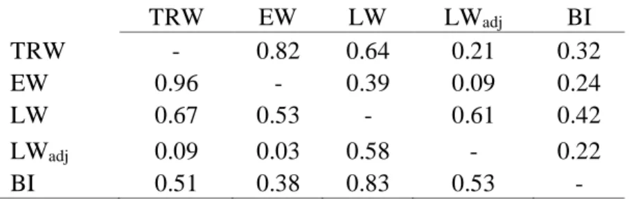
Table 2.3. Shared variance (r2) among PC1 metrics (lower-left of matrix) and among PC2 metrics (upper-right of matrix).
TRW EW LW LWadj BI
TRW - 0.82 0.64 0.21 0.32
EW 0.96 - 0.39 0.09 0.24
LW 0.67 0.53 - 0.61 0.42
LWadj 0.09 0.03 0.58 - 0.22
BI 0.51 0.38 0.83 0.53 -
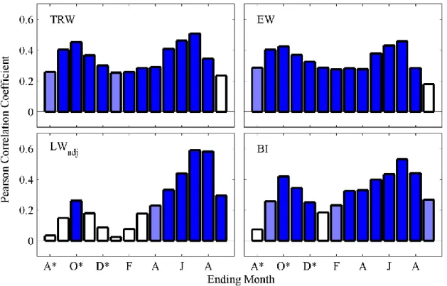
previous growing season, and some additional contribution from winter precipitation (Figure 2.2; full Seascorr results in Figure A5). For LWadj, the upper CRB chronologies primarily reflect summer precipitation (May through August) in the year of growth, with very little contribution from prior growing season conditions. The BI signal is similar to the ring width signals and primarily reflects warm-season precipitation in both the year of growth and the prior growing season. After accounting for the influence of precipitation on growth, there are generally low and non-significant correlations between maximum temperature and tree-ring metrics at these sites (Figure A5).
Figure 2.2. Pearson correlation coefficients between the first principal component of each tree-ring metric and 3-month precipitation composites (* = previous year). Dark blue shading indicates significance at a 99% level, and light blue shading indicates significance at a 95% level. Full Seascorr results (including correlations at different time-scales and with maximum temperature) are shown in Figure A5.
correlated with precipitation during the cool season and negatively correlated with warm-season precipitation. Seascorr results for TRW and EW chronologies at Sites 1 a nd 4 (not shown), which are both low elevation sites with positive loadings in PC2, differ substantially from the other sites. Whereas most sites correlate most strongly with warm-season
precipitation with little dependence on cool-season precipitation, Sites 1 and 4 are most strongly correlated with precipitation from the previous autumn through early spring. The negative correlation between warm-season precipitation and PC2 of TRW and EW may reflect a lack of warm-season precipitation dependence at Sites 1 and 4, in combination with additional warm-season precipitation dependence at Site 2, which has negative loadings in PC2. In contrast, PC2 of LWadj contains very little cool-season precipitation signal and instead reflects warm-season precipitation in the year of growth, similar to PC1 of LWadj. In general, PC2 of BI is not highly correlated to either cool-season or warm-season
Figure 2.3. Pearson correlation coefficients between the second principal component of each tree-ring metric and 3-month precipitation composites (* = previous year). Dark blue shading indicates significance at a 99% level, and light blue shading indicates significance at a 95% level. Full Seascorr results (including correlations at different time-scales and with maximum temperature) are shown in Figure A6.
Effective correlation analyses between Pcool and the 21 tree-ring metric composites indicate that the highest correlations (r = 0.56; Table 2.1) are achieved with a model that includes both PCs of TRW with no additional tree-ring metrics (Figure 2.4 a-b). In addition to being more parsimonious, the CPS model that includes only TRW is slightly more skillful (R2
vs = 0.12) than the four metric composite (R2vs = 0.11) and successfully captures more of the extremely dry cool seasons (EVClow = 0.7; p < 0.001) than the model that contains all four metrics (EVClow = 0.5; p < 0.01). CPS models based on EW, LWadj, or BI have no
reconstructive skill (R2
Figure 2.4. (a) Time plot of observed (grey) and predicted (black) October – March
precipitation (Pcool) in the CRB based on a CPS model of TRW (both PC1 and PC2). Dashed horizontal lines show thresholds for identification of years with extreme precipitation. (b) Scatter plot of observed Pcool and TRW-predicted Pcool. Filled circles indicate extreme years that were correctly identified (black) or not identified (gray) as extreme by the tree-ring CPS models. (c) Time plot of observed (grey) and predicted (black) May – August precipitation (Pwarm) in the CRB based on a CPS model of EW and LWadj (both PC1 and PC2). Dashed horizontal lines show thresholds for identification of years with extreme precipitation. (d) Scatter plot of observed Pwarm and predicted Pwarm. Filled circles indicate extreme years that were correctly identified (black) or not identified (gray) as extreme by the tree-ring CPS models.
Effective correlations between Pwarm and composites of ponderosa pine metrics (Table 2.2) indicate that warm-season precipitation is most strongly correlated with a composite containing both PCs of EW and LWadj (r = 0.66). While the individual metrics are each correlated with Pwarm with approximately equal strength (0.51 ≤ r ≤ 0.57), including TRW and BI along with EW and LWadj does not improve the overall correlation with Pwarm. As
suggested by the seasonal correlation analyses (Figures 2.2 and 2.3), the dominant signal in the network of CRB sites is related to warm-season precipitation, and the CPS skill for Pwarm therefore tends to be stronger than for Pcool. All COMBO composites exhibit at least some skill (R2
considerably more skillful than any individual metric. In contrast to the cool-season CPS tests, warm seasons that are extremely wet are successfully identified by most tree ring-based CPS models (EVChigh ≥ 0.4; p < 0.05). Warm seasons that are extremely dry are poorly reflected in the CPS-predicted Pwarm (EVClow ≤ 0.2; p > 0.05). While the variance explained by the CPS model declines when BI is added to the EW + LWadj composite, the proportion of extremely wet warm seasons that are correctly identified by the CPS model increases from 60% to 80%.
Discussion
Results from this research demonstrate that different tree-ring metrics contain different seasonal precipitation signals in the upper CRB, particularly in their sensitivity to cool-season and prior growing season precipitation, though the dominant signals tend to reflect dependence on warm-season precipitation. In some cases, combining tree-ring metrics with complementary signals improves CPS model skill. Total ring width of P. ponderosa
provides the strongest relationship to cool-season precipitation (r2 = 0.31; R2
vs = 0.12), and
including additional tree-ring metrics does not improve the CPS model of Pcool. However,
including multiple tree-ring metrics in a warm-season precipitation model offers substantial
gains in model strength: while the best single tree-ring metric explains 32% of Pwarm variance,
a model that includes both EW and LWadj explains 44% of Pwarm variance.
low elevation sites, which both have positive loadings in PC2 (Figures 2.3 and A2) and which are most strongly correlated with precipitation from autumn of the previous year through spring. The differences in precipitation signal between TRW/EW and LWadj may reflect the usage of stored photosynthate from the previous growing season for EW formation and the usage of photosynthate produced in the year of growth for LW formation [Kagawa et al., 2006; Offermann et al., 2011].
The signals embedded in these sub-annual ponderosa pine metrics differ from those found in other regions. In parts of the U.S. Southwest, for example, EW primarily reflects cool-season precipitation while LW tends to reflect warm-season precipitation delivered via the North American monsoon system [Meko and Baisan, 2001; Stahle et al., 2009; Griffin et al., 2013]. While previous studies have documented significant relationships between BI and warm-season temperature [McCarroll et al., 2011; Rydval et al., 2014; Wilson et al., 2014], I found very little evidence of temperature dependence in the BI chronologies from the upper CRB (after accounting for the variance explained by precipitation).
The precipitation–tree growth relationships found in this study (r2 = 0.31 for P
cool; r2 =
0.44 for Pwarm) compare favorably to those found in other studies of P. ponderosa in
northwestern North America, where precipitation typically explains anywhere from 20 -50%
of total ring width variance depending on site and season of interest [Graumlich, 1987;
Kusnierczyk and Ettl, 2002; Knutson and Pyke, 2008; Knapp and Soulé, 2011; Soulé and
Knapp, 2011]. It is possible that model strength could be further improved through inclusion
of tree-ring chronologies from other sites and species. Cool-season precipitation
reconstructions in particular may benefit from inclusion of subalpine conifer species such as
subalpine fir (Abies lasiocarpa) and mountain hemlock (Tsuga mertensiana) that are
negatively correlated with winter precipitation and spring snowpack [Peterson and Peterson,
developed in this study, Douglas-fir (Pseudotsuga menziesii) chronologies in northwestern
North America are often strongly correlated with warm-season precipitation [Watson and
Luckman, 2001; Littell et al., 2008; Lo et al., 2010; Crawford et al., 2015], but with slight
differences in seasonality [Watson and Luckman, 2002] which may complement the P.
ponderosa warm-season precipitation signal and improve reconstruction of Pwarm.
My results suggest that ponderosa pine metrics vary in their sensitivity to extreme precipitation in the U.S. Pacific Northwest. Among individual metrics, TRW successfully identifies 70% of extremely dry cool seasons, while LWadj only correctly identifies 10%. Likewise, CPS models based on LWadj are able to successfully identify 70% of extremely wet warm seasons, but none of the other three metrics correctly identify more than 50%. Tree ring-based predictions of warm-season precipitation are able to skillfully identify extremely wet years but not extremely dry years, while predictions of cool-season precipitation
successfully capture extremely dry years but not extremely wet years. This suggests that inferences regarding extreme events from these models or comparison between extremes in the instrumental and paleoclimate records would be stronger for extremely wet years in the warm season but stronger for extremely dry years in the cool season. Asymmetries in the ability to capture extreme events may stem in part from asymmetries in the distributions of precipitation itself. For example, the distribution of warm-season precipitation (Figures 2.4 c-d) is highly skewed, with most years clustered near the lower end of the precipitation
distribution. It may therefore be more difficult for tree-ring-based models to distinguish the driest years, which may be only slightly drier than other years that are not identified as extreme based on a 10% threshold. On the other hand, the wettest years are clearly separated from the bulk of the distribution and may therefore be easier to identify using tree-ring data since they are more distinct from the climatological norm. Quantifying the ability of
delineation of these strengths, weaknesses, and asymmetries in extreme value capture [McCarroll et al., 2015].
Summary and Conclusions
Seasonal biases in tree-ring records remain a major challenge for the reconstruction and interpretation of past climates, particularly in the U.S. Pacific Northwest [Steinman et al., 2012]. Previous studies have highlighted significant potential for improving seasonal climate reconstructions using combinations of multiple tree-ring metrics, including traditional TRW, sub-annual ring widths, and proxies for tree-ring latewood density. Using a network of TRW, EW, LWadj, and BI chronologies from six Pinus ponderosa sites in and surrounding the upper CRB, I examined the sensitivities of these four ponderosa pine metrics to seasonal climate variability and evaluated the potential for sub-annual precipitation reconstruction using multiple metrics in the U.S. Pacific Northwest.
I found that all ring-width indices in this region are sensitive to warm-season
growing season). Unlike previous studies in Scandinavia [McCarroll et al., 2011] and British Columbia [Wilson et al., 2014], I did not find a strong relationship between BI and
temperature in my semi-arid study region.
Effective correlation analyses and CPS tests suggest that use of multiple tree-ring metrics may improve seasonal precipitation reconstructions, though the magnitude of improvement may differ depending on the season of interest. In my study area, for example, TRW alone can explain more cool-season precipitation variance than all metrics combined. A composite index of EW and LWadj explains substantially more variance in warm-season precipitation than any single metric, thus highlighting the potential to capture seasonal climate signals embedded in sub-annual ring widths that are not resolvable by TRW alone. CPS tests suggest that reconstructions of Pcool and Pwarm in the upper CRB are asymmetric in their ability to capture extreme events. While CPS-predicted Pcool successfully identifies extremely dry years, there is very little skill in predicting extremely wet years. In contrast, the CPS model skillfully predicts extremely wet warm seasons, but not extremely dry ones. This asymmetry in the ability of CPS models to capture precipitation extremes suggests that future paleoclimate studies from other proxy records may benefit by using EVC as a validation metric to formally test the ability of variance-scaled reconstructions to correctly identify extreme events. Seasonal climate reconstruction and the capture of extremes in the tree-ring record may also benefit from future research to include stable isotope ratios of tree-ring cellulose as an additional metric and from the inclusion of chronologies from multiple species.
pressure deficit, pose significant threats to vegetated ecosystems that rely on winter
snowpack for soil moisture recharge [Boisvenue and Running, 2010; Williams et al., 2013]. Substantial uncertainties in the responses and feedbacks of vegetation to the impacts of climate change limit our ability to project future changes in the distribution and functioning of terrestrial ecosystems. Empirical studies on the responses of tree growth to historical variation of temperature and water availability can constrain these models and improve our understanding of the potential responses of forest ecosystems to climate change [Moorcroft, 2006]. While tree growth at the six sites used in this study seems to be primarily limited by summer water availability, there is substantial variation among sites in their reliance on winter precipitation. Growth at Sites 1 and 4, for example, is significantly related to precipitation from the previous autumn through early spring. These results suggest that the impacts of shifting precipitation seasonality, as expected under a changing climate, on the forests of the U.S. Pacific Northwest will likely vary geographically due to differential reliance of forests on precipitation from different seasons. Where tree growth is primarily dependent on summer precipitation, as in most of my study sites, redistribution of
CHAPTER 3: ENVIRONMENTAL STRESSES TO PRIMARY PRODUCTION IN THE CONTERMINOUS UNITED STATES
Introduction
Terrestrial primary production—the amount of carbon sequestered by plants via photosynthesis—is the fundamental source of food for all land-dwelling organisms and the primary entry point of energy and carbon into ecosystems. Recent estimates suggest around 80% of available primary production has already been appropriated for human use, with the remainder representing a key “planetary boundary” for future human activity [Running, 2012]. Terrestrial primary production is also a major component of the global carbon cycle, which has historically acted as a large sink for human emissions of CO2 [Pan et al., 2011; Ciais et al., 2013].
Many environmental factors plays an important role in regulating the growth and productivity of terrestrial vegetation, including climate, soil quality, and ecological processes (e.g., disturbance, competition, and succession) [Chapin et al., 2011]. Productivity of
production at a range of spatial and temporal scales is therefore crucial for modeling and monitoring primary production and for projecting responses of plant growth and productivity to future climate change.
The complexity of environmental limitations to plant growth—as well as their interactions with each other and their importance over different spatial and temporal scales— adds considerable uncertainty to models that attempt to monitor primary production based on satellite data. The dominant paradigm for modeling primary production with remote sensing is light-use efficiency (LUE) theory, which estimates plant production as a function of the amount of absorbed photosynthetically active radiation (PAR) by plant canopies and their efficiency at converting absorbed PAR to carbohydrates [Monteith, 1972, 1977, Song et al., 2013, 2015]. Many of these models assume a constant optimal LUE that is reduced in
response to “environmental stresses,” which are typically based on relatively simple functions of easily measured meteorological variables, such as temperature and vapor pressure deficit.
drive light-use efficiency, inclusion of soil quality factors in LUE models could lead to substantial improvements in primary production estimates [Nightingale et al., 2007], though soil data availability and quality would likely present a challenge for large-scale
implementation.
Given the limitations of current environmental stress models, in this chapter I develop an alternative approach for quantifying environmental stress effects on forest primary
production using tree-ring data and examine the drivers and seasonality of environmental stresses to forest primary production in the conterminous U.S. Widths of tree rings are a direct indicator of the net primary production that is allocated to woody growth [Graumlich et al., 1989; Rathgeber et al., 2000], and the sensitivity of stomatal, photosynthetic, and cambial processes to variation in each tree’s local environment make tree-ring widths ideal indicators of long-term variation in forest productivity and environmental stress [Fritts, 1976]. Recent studies have demonstrated significant potential for using tree-ring metrics as indicators of ecosystem-scale productivity [Beck et al., 2013; Bunn et al., 2013], suggesting that carbon cycle models (including those based on remotely sensed data) may benefit from assimilation of tree rings [Babst et al., 2014].
forest growth in the conterminous U.S., including stresses induced by unfavorable climatic, topographic, and edaphic conditions.
Data and Methods
A Tree-Ring Based Environmental Stress Index
At its core, “environmental stress” is the reduction of plant growth below optimal levels in response to inadequate resource availability or unfavorable ambient conditions. Where measurements of annual tree growth are available, the effects of environmental stress can therefore be represented as the ratio between the actual, measured diameter growth in a given year and the theoretical optimal diameter growth rate in that same year. While actual tree growth is easily measured using standard dendrochronological procedures, optimal growth is a theoretical construct that cannot be directly measured but must be estimated using species-specific allometric equations such as those used in forest gap models [e.g., Botkin et al., 1972; Shugart, 1984; Urban et al., 1993; Song and Woodcock, 2003]. The approach used here is the inverse of typical gap model applications: while I am estimating the impacts of environmental stress using actual measurements of tree growth, forest gap models typically simulate growth and succession of forests based on modeled environmental stresses (e.g., light, nutrients, and water availability).
To estimate the optimal growth of a given tree in a given year, I follow the approach originally proposed for the JABOWA gap model [Botkin et al., 1972]:
∆𝐷𝑜𝑝𝑡 =
𝐺𝐷[1−𝐷𝐻/𝐷𝑚𝑎𝑥𝐻𝑚𝑎𝑥]
274+3𝑏2𝐷−4𝑏3𝐷2 , (1)
Where ∆𝐷𝑜𝑝𝑡 is the optimal diameter growth (in cm) for a given tree in a given year, 𝐺 is a
species-specific allometric parameters. This formula assumes: 1) that annual volume increment is proportional to canopy leaf area (which is itself proportional to stem sapwood area), and 2) that there is an increasing maintenance cost with increasing tree size (i.e., as 𝐷 approaches 𝐷𝑚𝑎𝑥, volume increment approaches zero) [Botkin et al., 1972; Shugart, 1984]. I estimated
𝐷𝑚𝑎𝑥, 𝐻𝑚𝑎𝑥, and maximum age based on the maximum observed DBH, height, and age for each species provided in Hardin et al. [2001], supplemented with information from the gap model literature [Shugart, 1984; Urban et al., 1993]. I estimated the remaining parameters (𝐺, 𝑏2, and 𝑏3) using equations provided in Shugart [1984]. A full list of species and parameters used in this model is provided in Table A4.
For application to tree-ring datasets, where in situ measurements of DBH are not typically available, 𝐷 must be estimated using an “inside-out” approach, in which stem diameter at the start of a given year is estimated by summing all diameter increments prior to that year (𝐷∗). 𝐷∗ can then be substituted for 𝐷 in eqn. 1, resulting in an estimated optimal growth rate (∆𝐷𝑜𝑝𝑡∗ ). Estimating diameters in this manner will systematically underestimate
annual stem diameters, which I address below. As in many gap models, I estimate 𝐻 as a species-specific quadratic function of 𝐷∗.
Following estimation of ∆𝐷𝑜𝑝𝑡∗ , the environmental stress index, 𝑆∗, for a given year is estimated for each tree as the ratio of measured diameter growth (∆𝐷) to the estimated optimal diameter growth rate:
𝑆∗ = ∆𝐷
∆𝐷𝑜𝑝𝑡∗ . (2)
environmental stress experienced by trees, including both interannual variation in stress resulting from climate variability as well as perennial sources of stress resulting from unfavorable site conditions (e.g., steep slopes or poor soil nutrient status).
For comparison, I also define a relative stress index (𝑆𝑟) using methods standard to dendrochronology. Following typical detrending methods, I fit stiff smoothing splines (two-thirds the length of the series with a 50% frequency response) to the measured ring widths from each individual core, and divided this fitted curve into the measured ring width series to obtain a detrended ring width index [Cook, 1985]. As with 𝑆∗, I averaged the detrended ring width index series at each site using Tukey’s biweight robust mean to obtain site-level 𝑆𝑟,
retaining only the portions of the time-series that exceed an EPS of 0.85 [Wigley et al., 1984]. Unlike 𝑆∗, this relative stress index has the same mean across all sites and only represents the
interannual variation in stress experienced by trees. It therefore cannot capture spatial gradients in stress resulting from perennial reductions in growth due to unfavorable site conditions, but it also does not suffer from uncertainties introduced by the optimal growth model.
Tree-Ring Data
I tested the errors introduced to ∆𝐷𝑜𝑝𝑡∗ and 𝑆∗ due to systematic underestimation of annual DBH using increment cores collected at six semi-arid ponderosa pine sites in the U.S. Pacific Northwest (Chapter 2; Figure A9), where DBH was measured for each tree at the time it was sampled. Cores were collected, processed, and cross-dated following standard