Continuous Optimization Methods for
the Quadratic Assignment Problem
Tao Huang
A dissertation submitted to the faculty of the University of North Carolina at Chapel Hill in partial fulfillment of the requirements for the degree of Doctor of Philosophy in the Department of Statistics and Operations Research.
Chapel Hill 2008
Approved by:
Jon W. Tolle
J. Scott Provan
David S. Rubin
Vidyadhar G. Kulkarni
c
2008 Tao Huang
Abstract
TAO HUANG: Continuous Optimization Methods for the Quadratic Assignment Problem
(Under the direction of Jon W. Tolle)
In this dissertation we have studied continuous optimization techniques as they are
applied in nonlinear 0-1 programming. Specifically, the methods of relaxation with a
penalty function have been carefully investigated. When the strong equivalence
proper-ties hold, we are guaranteed an integer solution to the original 0-1 problem. The quadratic
assignment problem (QAP) possesses such properties and consequently we have
devel-oped an algorithm for the QAP based on the method of relaxation using the quadratic
penalty function. In our algorithm we have applied two pre-conditioning techniques that
enables us to devise a scheme to find a good initial point and hence obtain good solutions
to the QAP. Furthermore, we have shown how quadratic cuts can be used to improve
on the current solutions. Extensive numerical results on several sets of QAP test
prob-lems (including the QAPLIB) have been reported and these results show our algorithm
Acknowledgements
For many pursuing a doctoral degree is probably a pure academic endeavor, requiring
prolonged and dedicated efforts in a graduate program. My own pursuit has crossed
beyond that. Jiggling between a full-time job, family responsibilities and school has
proved very challenging to me. Along my journey there were many to whom I felt truely
indebted; if it were not for them I would have never come to where I am now. As I come
to the end of this journey, I would like to take this opportunity to express my sincere
gratitude to them.
Foremost, I would like to thank Him for answering many of my prayers and for
being a source of ideas and guidance. I am grateful to my wife, Ping, and sons, Teddy
and Ethan, for their patience, understanding, and sacrifice during many lost evenings
and weekends. I only feel relieved now I can finally fulfill my overdue promise to take
my son, Teddy, to soccer practice. I am also indebted to my parents for their silent and
unconditional support during the entire process.
I thank my advisor, Dr. Jon Tolle, for the opportunity to work on such an
interest-ing, although very challenginterest-ing, problem, and for his patience and guidance that helped
me complete this dissertation. My thanks also go to the rest of my dissertation
commit-tee members: Drs. J.S. Provan, D.S. Rubin, V.G. Kulkarni, and S. Lu for their time and
suggestions.
Last but not the least, I offer my deepest thanks to my friends whose names I do
Table of Contents
List of Figures . . . ix
List of Tables . . . x
1 Introduction . . . 1
1.1 Background . . . 1
1.1.1 Applications . . . 2
1.2 Alternative Formulations . . . 6
1.2.1 Quadratic 0-1 Programming Formulation . . . 6
1.2.2 Trace Formulation . . . 7
1.2.3 Kronecker Product . . . 9
1.3 Theoretical Complexity . . . 9
1.3.1 Other NP-Complete Problems as the Special Cases . . . 10
1.4 Published QAP Test Problems . . . 11
1.5 Practical Complexity . . . 13
1.6 Asymptotic Behavior . . . 14
1.7 Synopsis of the Remaining Chapters . . . 16
2 Nonlinear 0-1 Programming . . . 17
2.1 Formulations . . . 17
2.2 General Solution Approaches . . . 19
2.2.1 Linearization Methods . . . 19
2.2.2 Algebraic Methods . . . 20
2.2.3 Enumerative Methods . . . 21
2.2.4 Cutting-Plane Methods . . . 22
2.4 Methods for the Quadratic Assignment Problem . . . 25
2.4.1 Branch-and-Bound Methods . . . 25
2.4.2 Lower Bounds . . . 26
3 Methods of Relaxation with a Penalty Function . . . 30
3.1 Introduction . . . 30
3.2 General Weak Equivalence . . . 34
3.3 Relaxation Using the Quadratic Penalty Function . . . 37
3.4 Strong Equivalence of the QAP Relaxation . . . 43
3.5 A Smoothing Algorithm . . . 45
3.6 Asymptotic Properties of the Quartic Penalty Function . . . 48
3.7 Summary . . . 57
4 Solving the QAP via Relaxation and Quadratic Cuts . . . 60
4.1 Overview . . . 60
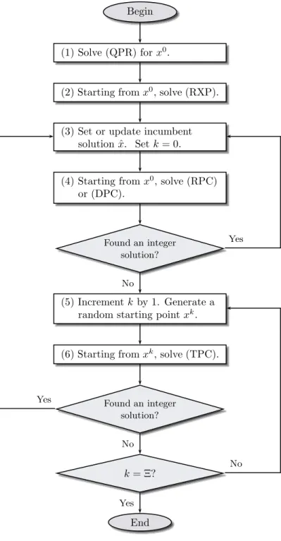
4.1.1 The Algorithmic Framework . . . 61
4.2 Convex Transformation of the Objective Function . . . 64
4.2.1 Motivation . . . 64
4.2.2 Techniques of Convex Transformation . . . 65
4.3 Pre-Conditioning the Hessian of the Objective Function . . . 66
4.3.1 Motivation . . . 66
4.3.2 Minimizing the Spread of Eigenvalues . . . 68
4.3.3 Bounding the Condition Number of the Hessian . . . 76
4.4 Formulating the Relaxation Problems with Quadratic Cuts . . . 82
4.5 Random Starting Points for the Quartic Penalty Problems . . . 83
5 Algorithm Implementation and Numerical Results . . . 87
5.1 Implementation Details . . . 87
5.1.1 Solving Optimization Problems Using IPOPT . . . 87
5.1.2 Approximating the Hessian with an L-BFGS Update . . . 89
5.1.3 Solving (RPC) vs. (DPC) . . . 91
5.1.4 Solving (TPC) Efficiently . . . 91
5.1.5 Initial Interior Point for the Symmetric Mixing Algorithm . . . . 94
5.2 Results on the QAPLIB Instances . . . 96
5.3 Results on Other Published QAP Test Problems . . . 101
5.4 Summary of Numerical Results . . . 107
6 Conclusions, Further Research and Extensions . . . 108
6.1 Conclusions . . . 108
6.2 Further Research and Extensions . . . 108
A Proofs from Literature . . . 110
A.1 Total Unimodularity of the Assignment Matrix . . . 110
A.2 Proof of Proposition 3.6 . . . 111
B Test Problems and Numerical Results . . . 112
B.1 QAPLIB Instances . . . 112
B.2 Results of Matrix Reduction Algorithm . . . 113
B.3 Results of Scaling and Shift Algorithm . . . 116
List of Figures
1.1 Backboard Configuration . . . 3
3.1 Proof of Weak Equivalence . . . 35
3.2 A Simple Problem with a Convex Quadratic Objective Function . . . 40
3.3 Parameterized Objective Function in One-Dimensional Relaxation . . . 41
3.4 Illustration of Smoothing Algorithm in Two-Dimensional Subspace . . . 47
4.1 Flowchart of the Algorithmic Framework . . . 62
4.2 Contours of Convex Quadratic Functions . . . 67
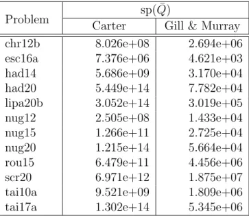
4.3 Spreads of Eigenvalues of ¯A and ¯B . . . 74
4.4 Minimization for γ and σ . . . 79
List of Tables
1.1 Hospital Layout – Facilities and Their Functions . . . 4
1.2 Hospital Layout – Flow and Distance Matrices . . . 5
1.3 Recently Solved Large QAPLIB Instances . . . 13
4.1 Comparison of Carter’s and Gill and Murray’s Algorithms . . . 71
5.1 Exact Hessian vs. L-BFGS Approximation . . . 90
5.2 Quadratic Cut: Solving (RPC) vs. (DPC) . . . 92
5.3 Solving Multiple Instances of (TPC) with LBFGS . . . 93
5.4 Results on the QAPLIB Instances with N <100 . . . 96
5.5 Comparison on Recently Solved Large QAPLIB Instances . . . 101
5.6 Results on the Instances by Drezner et al. with N <100 . . . 102
5.7 Results on the Instances by Palubeckis with N <100 . . . 103
5.8 Results on the Instances by St¨utzle and Fernandes with N <100 . . . 104
B.1 A Complete List of the QAPLIB Instances . . . 112
B.2 Matrix Reduction Algorithm on QAPLIB Instances with N ≤100 . . . 114
Chapter 1
Introduction
1.1
Background
Consider a situation where we have N facilities and N locations, and we are to assign
each facility to a location. For a possible assignment, there is a cost associated with each
pair of facilities which is proportional to both the flow and the distance between the pair.
There is also a cost of placing a facility at a certain location. Our objective is to assign
the facilities to the locations such that the total cost is minimized. Specifically, suppose
we are given a setN ={1,2, . . . , N}, a flow matrixF = (fij)∈RN×N, a distance matrix
D= (dkl)∈ RN×N, and a fixed cost matrix C = (cik)∈ RN×N, where fij represents the cost associated with transporting the commodities over a unit distance from facility ito
facility j,dkl is the distance from locationk to locationl, andcik is the cost of assigning
facility i to location k. The problem can be formulated as follows.
(1.1) minimize
π∈ΠN
N
X
i=1
N
X
j=1
fijdπ(i)π(j)+
N
X
i=1
ciπ(i)
where ΠN is the set of all the permutations of N. The product fijdπ(i)π(j) is the cost
of simultaneously assigning facility i to location π(i) and facility j to location π(j).
Although in the context of facility to location assignments the distance matrixDis almost
always symmetric, in a more general setup no assumption is made on the symmetry of
the matrices F and D.
Problem (1.1) is known as the quadratic assignment problem (or QAP for short).
It was originally introduced in 1957 by Koopmans and Beckmann [70]. Koopmans and
Beckmann derived the QAP as a mathematical model to study the assignment of a set of
economic activities to a set of locations. Since then the QAP has been a subject of
importance, but also because of its complexity. With the advent of high performance
computing capability, we have seen a large number of formerly intractable combinatorial
problems that have become practically solvable in the last decade. Unfortunately, the
QAP is not among those problems. In general, QAP instances of size N ≥ 20 are still considered intractable. The QAP remains one of the most challenging combinatorial
problems from both a theoretical and a practical point of view.
For recent comprehensive surveys of various aspects of the QAP, the reader is
re-ferred to Anstreicher [4], Burkard and C¸ ela [18], Burkard et al. [19], C¸ ela [27], Finke et
al. [33], and Pardalos et al. [92].
To facilitate the discussion, we will denote a QAP instance with a flow matrix F,
distance matrix D, and cost matrix C by QAP(F, D, C). When C = 0, we denote the
instance by QAP(F, D).
1.1.1
Applications
The QAP initially occurred as a facility location problem, which remains one of its
ma-jor applications. In addition, the QAP has found applications in other areas such as
scheduling [40], manufacturing [51], parallel and distributed computing [13],
combina-torial data analysis [63], ergonomics [81, 96], archaeology [71], and sports [61]. In the
following we briefly describe two applications that will shed insight into the applicability
and significance of the QAP.
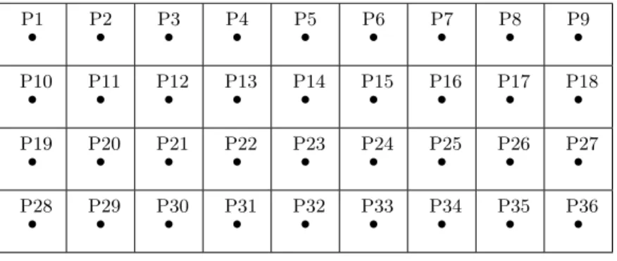
Steinberg Wiring Problem. This early application is due to Steinberg [106] who gave a detailed account of computer backboard wiring problems. Given a set E =
{E1, E2, . . . , Em} of m electronic components, we require Ei to be connected to Ej by
Wij wires. Hence we have a symmetric connection matrix W = (wij) with its diagonal
elements wii = 0, i = 1,2, . . . , m. In addition, there are r points P1, P2, . . . , Pr on the backboard, where r≥ m. Let dkl be some distance measure that may be interpreted as the length of wire needed to connect two electronic components if one is placed at Pk
and the other is placed at Pl. Hence we obtain a symmetric distance matrix D = (dkl)
with zeros down the diagonal. The most commonly used distance measures between two
points are the Euclidean distance and Manhattan distance, i.e., the`2-norm and `1-norm
respectively of a vector that emanates from one point and ends at the other. The goal is
P1
• P2• P3• P4• P5• P6• P7• P8• P9•
P10
• P11• P12• P13• P14• P15• P16• P17• P18•
P19
• P20• P21• P22• P23• P24• P25• P26• P27•
P28
• P29• P30• P31• P32• P33• P34• P35• P36• Figure 1.1 Backboard Configuration1
wire length needed is minimized. By introducing r−m fictitious electronic components with no wires running to or between them, we getrcomponents that have to be placed at
rpoints. Hence the backboard wiring problem becomes a quadratic assignment problem;
the connection matrix W becomes the flow matrix in problem (1.1).
As illustrated in Figure 1.1, Steinberg showed a section of the backboard of a
mod-ified Univac Solid-State Computer, on which 34 electronic components E1, E2, . . . , E34
were to be placed and connected. The dots P1, P2, . . . , P36indicate the possible positions
where the electronic components must be placed. The positions form a two-dimensional
grid and any two adjacent dots are at a distance of 1 unit both horizontally and
verti-cally. Steinberg provided the connection matrix W = (wij), for 1 ≤ i < j ≤ 34. In this example, two fictitious components E35 and E36 are added so that in every assignment
two positions will be empty.
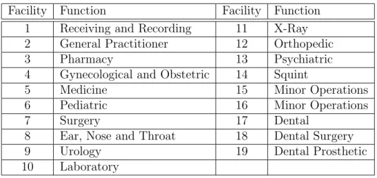
Hospital Layout. Elshafei [32] at the Institute of National Planning in Cairo, Egypt investigated a hospital layout problem in which several clinics of a public hospital in
Cairo were to be located so as to minimize the total distance that the patients had to
travel to receive treatment in the clinics. The problem resulted from a rapid increase
in the number of patients in the Outpatient department at the time. As a result, the
department became overcrowded with an average daily number of patients exceeding
700 and those patients having to move among its 17 clinics. The location of the clinics
relative to one another was criticized for causing too much travel by the patients and
1Copyright c1961 Society for Industrial and Applied Mathematics. Reprinted with permission from
Table 1.1 Hospital Layout – Facilities and Their Functions2
Facility Function Facility Function
1 Receiving and Recording 11 X-Ray
2 General Practitioner 12 Orthopedic
3 Pharmacy 13 Psychiatric
4 Gynecological and Obstetric 14 Squint
5 Medicine 15 Minor Operations
6 Pediatric 16 Minor Operations
7 Surgery 17 Dental
8 Ear, Nose and Throat 18 Dental Surgery
9 Urology 19 Dental Prosthetic
10 Laboratory
serious delays. Since the flow of the patients was confined between the receiving and
recording room and the 17 clinics, the study focused exclusively on the relative location
of these 18 facilities. All the facilities needed roughly the same area except for the Minor
Operations which occupied nearly twice as much space as any other facility. Hence the
Minor Operations section was split into two pseudo facilities that had to be placed side
by side. As in Table 1.1, there were 19 facilities to be considered in the layout planning.
As Elshafei stated, the estimates of the patient flows between the clinics were
avail-able on a yearly basis. Thus a symmetric flow matrix was obtained by averaging the flows
between each pair of facilities. The flow between the two pseudo facilities was assigned
a very large number such that their adjacency was forced. The distances between the
locations could be reasonably measured by tracing the paths of the patients moving from
one location to another; the resulting distance matrix therefore was symmetric. Thus the
hospital layout problem was formulated as a quadratic assignment problem. In Table 1.2
the lower triangular part shows the flows between the facilities and the upper triangular
part shows the distances between the locations.
Other applications of the QAP abound in the literature. For more references to
different applications of the QAP, the reader is referred to Burkard et al. [19], C¸ ela [27],
Pardalos et al. [92], and Padberg and Rajal [90].
1.2
Alternative Formulations
The quadratic assignment problem is often stated as (1.1). This is because problem (1.1)
readily reveals the combinatorial structure of the QAP. However, problem (1.1) is rarely
used in posing solution methods for the QAP. Instead, alternative formulations have been
suggested that allow for different solution approaches. In the following we discuss three
alternative formulations that are often cited in the literature.
1.2.1
Quadratic
0
-
1
Programming Formulation
We observe that there is a one-to-one correspondence between ΠN, the set of all the
permutations of N, and the set of N ×N permutation matrices X = (xij). To be specific, we have
(1.2) xij =
(
1 if facility i is assigned to locationj, i.e., π(i) =j;
0 otherwise.
X is a permutation matrix if and only if
N
X
j=1
xij = 1, i= 1, . . . , N, (1.3a)
N
X
i=1
xij = 1, j = 1, . . . , N, (1.3b)
xij ∈B, i, j = 1, . . . , N,
(1.3c)
where B={0,1}.
(1.3a) and (1.3b) are referred to as the assignment constraints and the coefficient
matrix of the assignment constraints referred to as the assignment matrix. With the
assignment constraints, we can formulate the QAP as the following quadratic 0-1
pro-gramming problem:
minimize N
X
i=1
N
X
j=1
N
X
k=1
N
X
l=1
fijdklxikxjl+ N
X
i=1
N
X
k=1
cikxik (1.4)
subject to (1.3a)–(1.3c).
Problem (1.4) is also called the Koopmans-Beckmann formulation because it was initially
The equivalence between problems (1.1) and (1.4) is obvious. The termfijdklxikxjl
contributes to the objective function only if xik =xjl = 1, i.e., if facility i is assigned to
location k and facilityj to location l. The term cik contributes to the objective function
only if facility i is assigned to locationk.
Note that the sum of the constraints in (1.3a) is equal to the sum of the constraints
in (1.3b). Hence the assignment constraints in (1.3a) and (1.3b) are linearly dependent.
It is easy to see that after deleting one of the assignment constraints, the remaining
assignment constraints are linear independent. Therefore, we can write (1.4) in a more
compact form using the matrix-vector notation:
minimize 12xTQx+cTx
(1.5)
subject to Lx=b
x∈Bn, where Q ∈ Rn×n with n = N2 is symmetric, c ∈
Rn, L ∈ Rm×n with m = 2N −1,
and b ∈ Rm is a vector of all ones. Note that the assumption on the symmetry of Q is valid because we can always substitute 12(Q+QT) for Q to achieve the symmetry if
Q is asymmetric. In this formulation Q and L have special structures. More generally,
(1.5) with arbitrary symmetric Q and L with full row rank is called a quadratic 0-1
programming problem.
1.2.2
Trace Formulation
For two N ×N matrices A and B, we have tr(ABT) =hA, Bi=
N
X
i=1
N
X
j=1
aijbij
where tr(·) denotes the trace of a matrix and h·,·i the inner product of two matrices. Given a permutation π ∈ΠN, the associated permutation matrix X as defined in (1.2), and a N ×N matrix D, XD is equivalent to a rearrangement of the rows of D in the order of π and DXT a rearrangement of the columns of D in the order of π. Therefore,
we have
XDXT = dπ(i)π(j)
,
tr(F XDTXT) =hF, XDXTi=
N
X
i=1
N
X
j=1
fijdπ(i)π(j),
and also
tr(CXT) = N
X
i=1
ciπ(i).
(1.7)
The following are some of the well-known properties of the traces of two matrices
A and B:
tr(A+B) = tr(A) + tr(B),
(1.8a)
tr(AB) = tr(BA), and (1.8b)
trA = trAT.
(1.8c)
From (1.8a), (1.6), and (1.7), the QAP of the form (1.1) can be written as
minimize tr(F XDT +C)XT
(1.9)
subject to X ∈ PN
wherePN is the set of allN×N permutation matrices. Furthermore, using the properties (1.8b) and (1.8c) we will show that if either F =FT orD =DT then
(1.10) tr(F XDTXT) = tr(F XDXT).
ForD =DT, (1.10) holds trivially. For F =FT but D6=DT, it follows that tr(F XDTXT) = tr(F XDTXT)T
= tr(XDXTFT)
= tr(XDXTF)
= tr(F XDXT).
Similarly we can show that if either F =FT or D=DT then
(1.11) tr(FTXDXT) = tr(F XDXT).
(1.10) and (1.11) suggest that we can reformulate a QAP instance in which either the flow
matrix or the distance matrix but not both are asymmetric into an equivalent instance
in which both matrices are symmetric. For example, in a case whereF is symmetric but
1.2.3
Kronecker Product
In the Koopmans-Beckmann formulation in (1.4), we can rewrite
N X i=1 N X j=1 N X k=1 N X l=1
fijdklxikxjl
as xT
f11d11 · · · f1Nd11 f11d1N · · · f1Nd1N ..
. . .. ... · · · ... . .. ...
fN1d11 · · · fN Nd11 fN1d1N · · · fN Nd1N
· · ·
· · ·
· · ·
f11dN1 · · · f1NdN1 f11dN N · · · f1NdN N ..
. . .. ... · · · ... . .. ...
fN1dN1 · · · fN NdN1 fN1dN N · · · fN NdN N
x
=xT
d11F · · · d1NF ..
. . .. ...
dN1F · · · dN NF
x=x
T(D⊗F)x
with x = vec(X) = x11· · ·xN1 · · · x1N· · ·xN N
T
. Here vec(·) denotes the vector formed by the columns of a matrix and ⊗ denotes the Kronecker product. Thus the QAP can be formulated as
minimize vec(X)T(D⊗F) vec(X) + vec(C)Tvec(X) (1.12)
subject to X ∈ PN.
Note that the Hessian of the objective function of the QAP isQ= 2D⊗F. One of the useful properties of a Kronecker product [48] is that the eigenvalues of the Kronecker
productD⊗F are theN2eigenvalues formed from all possible products of the eigenvalues of F and D. This will be used to compute the smallest and largest eigenvalues of Q in
Chapter 4.
1.3
Theoretical Complexity
Sahni and Gonzalez [103] have established the complexity of exactly and approximately
solving the QAP. Before we present their results, we introduce the following definition of
Definition 1.1 Given > 0, an algorithm is said to be an -approximation algorithm for the QAP if for every instance QAP(F, D),
Z∗(F, D)−Zˆ(F, D)
Z∗(F, D)
≤,
where Z∗(F, D) > 0 is the optimal objective value and Zˆ(F, D) is the objective value of the solution obtained by the algorithm. The solution obtained by an -approximation
algorithm is said to be an -approximation solution for the QAP.
Theorem 1.1 (Sahni and Gonzalez [103], 1976) The quadratic assignment problem is NP-complete. For an arbitrary >0, there does not exist a polynomial-time
-approx-imation algorithm for the QAP unless P=NP.
Although there exist polynomially solvable cases [19, 27] of the QAP where special
structural conditions hold on the coefficient matrices, Theorem 1.1 implies that in general
it is unlikely that a polynomial-time algorithm for the QAP will be found. Furthermore,
even finding an -approximation solution to the QAP is a very difficult problem.
1.3.1
Other NP-Complete Problems as the Special Cases
Several well-known NP-complete problems can be formulated as special cases of the
QAP. While the QAP is not a tractable problem, in practice no one would want to
use algorithms developed for the QAP to solve those NP-complete problems since the
specialized algorithms for solving those problems are far more efficient than any solution
method for the QAP. However, the relationship between the QAP and those problems
sheds light upon the inherent complexity of the QAP. In the following we present three
well-known combinatorial optimization problems as special cases of the QAP.
The Traveling Salesman Problem. We are given a set of N cities and pairwise distances between them, and our task is to find the shortest tour that visits each city
exactly once. Let {1,2, . . . , N} represent the N cities and the N ×N matrix D= (dij) the distances between the cities. We can formulate the traveling salesman problem as
the QAP with the distance matrix equal to D and the flow matrix being the adjacency
The Graph Partitioning Problem. Consider an edge weighted graph G = (V, E) with|V|=N and an integerk that dividesN. We are to partitionV intok sets of equal cardinality and meanwhile minimize the total weight of the edges cut by the partition. We
can formulate this problem as the QAP with the distance matrix equal to the weighted
adjacency matrix ofGand the flow matrix being−1 multiplying the adjacency matrix of a graph consisting of k disjoint complete subgraphs each of which has Nk vertices. Note
that 1) the sum of the elements of the weighted adjacency matrix ofGremains constant,
and 2) by formulating the problem as the QAP we effectively maximize the sum of the
elements of the weighted adjacency matrix of a union of k disjoint subgraphs of G, each
of which is induced by Nk vertices of G. Hence the QAP formulation is equivalent to
minimizing the total weight of the edges cut by the partition.
The Maximum Clique Problem. Suppose we have a graph G= (V, E) with |V|=
N. We would like to find a subset V1 of the largest cardinality such that V1 ⊆ V and
V1 induces a clique in G, i.e., all the vertices of V1 are connected by edges in G. Let
us consider the QAP with the distance matrix equal to the adjacency matrix of G and
the flow matrix given as −1 multiplying the adjacency matrix of a graph consisting of a clique of size k and N −k isolated vertices. Note that a clique of size k exists only if the QAP has an optimal objective value of −k2+k, i.e., the sum of the elements of the adjacency matrix of a clique of size k. The maximum clique can be found by solving a
series of N QAP instances for k= 1,2, . . . , N.
1.4
Published QAP Test Problems
Due to the increased research activities in the QAP, several sets of QAP test problems
have been proposed by the research community. These test problems provide a platform
on which various solution methods for the QAP can be evaluated or compared. In the
following we will discuss four sets of QAP test problems that are accessible to the research
community. We will use some of these instances to test our proposed algorithm for the
QAP in Chapter 5.
QAPLIB [22] Instances. The QAPLIB was first published in 1991 to provide a uni-fied test base for the QAP. This is the most commonly used set of test problems among
10 to 256. 4 out of the 137 instances have a size greater than 100. A complete list of
the QAPLIB instances with the objective values of the optimal or best known solutions
is given in Table B.1 in Appendix B.1. The QAPLIB instances and their solution
sta-tus have been made available via its website at http://www.seas.upenn.edu/qaplib/.
The online version is updated on a regular basis and contains the most current
informa-tion of the soluinforma-tion status. As of this writing, except for those with optima known by
construction, the largest instances that have been optimally solved have a size of 36.
Instances by Drezner, Hahn and Taillard [30]. Drezner, Hahn and Taillard pro-posed a total of 142 QAP instances with the sizes ranging from 12 to 729 and whose
characteristics are complementary to the QAPLIB instances. According to Drezner,
Hahn and Taillard, the QAPLIB instances are difficult for the exact methods but are
solved relatively easily by the heuristic methods within a fraction of one percent of the
optimal or best known solutions. The instances proposed by Drezner, Hahn and Taillard
were constructed in such a way that they are difficult for the heuristic methods but
in-stances of a size up to 75 are solved relatively easily by the exact methods in a reasonable
amount of time.
One of the measures for the difficulty of QAP instances is the landscape
rugged-ness [3], defined as the normalized variance of the difference between two neighboring
solutions. The variance is normalized such that the ruggedness is between 0 and 100,
with a larger value for a more difficult problem. For some of the instances proposed by
Drezner et al., the ruggedness is nearly 100.
Instances by Palubeckis [91]. Palubeckis proposed a set of 10 QAP instances with the sizes ranging from 20 to 200. Limited computational results show that these instances
are more difficult for the heuristics than some of the well-known QAPLIB instances.
Instances by St¨utzle and Fernandes [108]. St¨utzle and Fernandes proposed a to-tal of 644 instances with the sizes ranging from 50 to 500. This set of instances with
more varied characteristics than the other sets were constructed mainly for study of the
1.5
Practical Complexity
The advances in computer hardware in the last decade have brought about significant
progress in solving some of the most difficult combinatorial optimization problems. The
traveling salesman problem is an example. TSP instances with thousands of cities can
be solved in practice [27]. However, the QAP is an exception. It is generally considered
computationally difficult [6, 16, 22] to solve the QAP of modest sizes, say N ≥20. The QAP instances with N = 30 is roughly the current practical limit for the exact solution
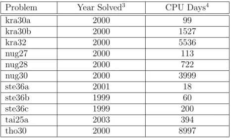
methods [4, 6]. Several problems from QAPLIB with aboutN = 30 that had been open
for decades were only recently solved. For the solution of the QAPLIB instance nug30 an
average of 650 computers were used over a one-week period, providing the equivalent of
almost 7 years of computation on a single HP9000 C3000 workstation [6]. The CPU time
used to solve the QAPLIB instance tho30 is equivalent to over 15 years of computation
on a single C3000. Table 1.3 lists the years in which the problems were exactly solved
and the CPU time spent for nearly a dozen recently solved large QAP instances from the
QAPLIB.
Table 1.3 Recently Solved Large QAPLIB Instances
Problem Year Solved3 CPU Days4
kra30a 2000 99
kra30b 2000 1527
kra32 2000 5536
nug27 2000 113
nug28 2000 722
nug30 2000 3999
ste36a 2001 18
ste36b 1999 60
ste36c 1999 200
tai25a 2003 394
tho30 2000 8997
Note that most of these successes were achieved in the distributed computing
en-vironments where massive networks of computers were utilized to meet the daunting
3These data are excerpted from the QAPLIB website.
computational demand.
1.6
Asymptotic Behavior
The QAP exhibits an interesting asymptotic behavior. As outlined below, if certain
probabilistic conditions on the problem data are satisfied, the ratio of its best and worst
objective values approaches 1 as the problem size goes to infinity. On one hand, this
behavior suggests that the error of any heuristic method vanishes as the problem size
tends to infinity. That is, if the problem size is large enough, the QAP becomes a trivial
problem in the sense that every heuristic method finds an almost optimal solution. On
the other hand, as the problem size increases, all the feasible solutions to the QAP are
clustered between two level sets of the objective function that become arbitrarily close.
This renders an exact algorithm such as the branch and bound method very inefficient.
In this situation the branch and bound method tends to enumerate a majority of the
nodes in the branch and bound tree unless arbitrarily tight lower bounds are available.
This behavior will also cause difficulty for the continuous optimization methods that we
use in this research. Due to the clustering of the feasible points as the problem size
increases, our algorithm using the continuous optimization methods may not be able to
“distinguish” between the good and bad solutions and hence may fail to find a good
solution.
In an early work Burkard and Fincke [20] studied the difference between the best
and worst objective values of some special cases of the QAP. They first considered the
planar QAP, where the distance matrix consists of pairwise distances between the points
chosen independently and uniformly from the unit square in the plane and the flows are
independent random variables on [0,1]. Then they investigated the QAP where both the
flows and the distances are independent random variables on [0,1]. In both cases they
showed that the difference between the best and worst objective values approaches 0 with
a probability tending to 1 as the problem size goes to infinity.
Later Burkard and Fincke [21] investigated the asymptotic behavior of a generic
combinatorial optimization problem. They considered a sequence PN, N = 1,2, . . .,
of minimization problems with a sum objective function as described below. For each
f :FN 7→R was defined as
(1.13) f(X) = X
x∈X
cN(x)
for allX∈ FN. Burkard and Fincke showed that the ratio of the best and worst objective values of (1.13) converges to 1 in probability as N → ∞. Szpankowski [109] improved the order of convergence by showing that the convergence holds almost surely. In the
almost sure convergence the probability that the ratio of the best and worst objective
values approaches 1 is equal to 1.
C¸ ela [27] showed that the QAP is a special case of combinatorial optimization
prob-lems with a sum objective function. More specifically, it was shown that the ground set
is SN = {(i, j, k, l) : 1 ≤ i, j, k, l ≤ N}. Each permutation π of N corresponds to a
feasible solution Xπ as a subset of SN, Xπ = {(i, j, π(i), π(j)) : 1 ≤ i, j ≤ N}. The set FN of the feasible solutions consists of all feasible solutions Xπ for π ∈ ΠN. The cost function is given as cN(i, j, k, l) = fijdkl. Based on the work of Burkard and Fincke [21]
and Szpankowski [109] for general combinatorial problems, C¸ ela obtained the following
theorem.
Theorem 1.2 (C¸ ela [27], 1998) Consider a sequence of QAP(FN, DN) with N ×N
flow and distance matrices FN = (fN
ij) and DN = (dijN). Assume that for M >0 the fijN
and, distinctly, the dN
ij are identically and independently distributed random variables on [0, M] with finite first, second, and third moments. LetZmin and Zmaxdenote the optimal
and worst objective values of QAP(FN, DN), respectively:
Zmin = min
π∈ΠN
N
X
i=1
N
X
j=1
fijNdNπ(i)π(j)
Zmax = max
π∈ΠN
N
X
i=1
N
X
j=1
fijNdNπ(i)π(j)
Then the following holds almost surely:
lim N→∞
Zmin
Zmax
= 1.
Several other authors obtained different analytical forms of the asymptotic
behav-ior of the QAP by imposing slightly different probabilistic conditions. The readers are
Frenk, Houweninge and Rinnooy Kan [37] conduct computational experiments to
empirically verify the asymptotic property of the QAP. Their results confirm that the
ratio converges to 1 relatively quickly. For the examples they use, the ratio falls within
0.1 of its theoretical value from approximately N = 50 onwards.
1.7
Synopsis of the Remaining Chapters
In Chapter 2 we will survey the literature on the solution approaches for nonlinear 0-1
programming. As special cases of nonlinear 0-1 programming, we will also survey the
solution methods specific for quadratic 0-1 programming and the QAP. In Chapter 3
we will study the methods of relaxation with penalty functions. We will discuss the
properties of weak and strong equivalence of the relaxation using two penalty functions.
The asymptotic properties of the relaxation using the quartic penalty function will also
be discussed. Based upon the method of relaxation using the quadratic penalty function,
we will propose an algorithm for the QAP in Chapter 4. We will describe two important
techniques used in our algorithm, i.e., the convex transformation of the objective function
of the QAP and the pre-conditioning the Hessian of the objective function. Then we
will show how quadratic cuts can be applied to improve the solutions to the QAP. In
Chapter 5 we will describe the implementation details of our algorithm for the QAP.
Then we will show and discuss the numerical results of our algorithm on the QAPLIB
instances and other published QAP test problems. We will draw conclusions and discuss
possible extensions of our algorithm for the QAP to quadratic 0-1 programming and
Chapter 2
Nonlinear 0-1 Programming
In this chapter we will present a brief overview of formulations of nonlinear 0-1
pro-gramming and its main solution approaches reported in the literature. The quadratic
assignment problem, the focus of this dissertation, is a special case of quadratic 0-1
programming which in turn is a subclass of nonlinear 0-1 programming. Hence in
prin-ciple we could solve the quadratic assignment problem as a nonlinear 0-1 programming
problem. We will also give a brief summary of the extensive literature in the solution
techniques for quadratic 0-1 programming. Last we will discuss the methods to solve the
quadratic assignment problem.
2.1
Formulations
To simplify the notation but without loss of generality, we consider a nonlinear 0-1
programming problem of the following form
minimize f(x) (2.1)
subject to g(x)≤0
x∈Bn
where f : Rn 7→
R, g : Rn 7→ Rm, and B = {0,1}. Since any equality constraint can
be replaced by two equivalent inequality constraints, this form includes the cases with
equality constraints and the QAP can be viewed as a special case of it.
Problem (2.1) is important in its own right. For a list of references to the applications
of nonlinear 0-1 programming, see Balas and Mazzola [9], Boros and Hammer [15], and
Hansen et al. [60]. In addition, an integer or mixed-integer nonlinear programming
programming problem by binary expansions. In particular, we can replace an integer
variable y with bounds l ≤y ≤uby the following:
y=l+x1+ 2x2+ 4x3+· · ·+ 2K−1xK where xi ∈B fori= 1, . . . , K and K is given by
K =blog2(u−l)c+ 1.
It is shown in Hammer and Rudeanu [58] that any function in 0-1 variables can be
reduced to a polynomial in the same variables. Indeed, if we set
∆i(x1, . . . , xi−1, xi+1, . . . , xn) (2.2)
=f(x1, . . . , xi−1,1, xi+1, . . . , xn)−f(x1, . . . , xi−1,0, xi+1, . . . , xn), and
ηi(x1, . . . , xi−1, xi+1, . . . , xn) = f(x1, . . . , xi−1,0, xi+1, . . . , xn), (2.3)
it is easy to verify that
(2.4) f(x1, . . . , xn) =xi∆i(x1, . . . , xi−1, xi+1, . . . , xn) +ηi(x1, . . . , xi−1, xi+1, . . . , xn). Applying (2.4) recursively, we can reduce (2.1) to the following polynomial 0-1
program-ming problem:
minimize f(x) = p0
X
k=1
ck
Y
j∈Nk
xj (2.5)
subject to pi
X
k=1
aik
Y
j∈Nik
xj ≤bi, i= 1,2, . . . , m
x∈Bn
where Nk ⊆ N = {1,2, . . . , n}, k = 1,2, . . . , p0 and Nik ⊆ N, k = 1,2, . . . , pi, i = 1,2, . . . , m. Note that the propertyx2
j =xj,∀j, implies all variables have a power of 1 in the terms in which they appear. (2.5) is also called multilinear 0-1 programming.
Moreover, Rosenberg [101] has shown that any unconstrained polynomial 0-1
pro-gramming problem minimizex∈Bnf(x) can be reduced to the quadratic case. We replace
all occurrences of a product of two variables xixj appearing in the terms of order greater
than two in f(x) by a new variable xn+l and then add the following corrective term in the objective function
for some µ >f˜−f where ˜f is the value of f(x) at some x∈Bn and f is a lower bound onf(x) on Bn, given asf =Pp0
k=1min(0, ck). Note that (xixj+ (3−2xi−2xj)xn+l) = 0 for xn+l = xixj and (xixj + (3−2xi−2xj)xn+l) ≥1 otherwise. Hence any solution for which xn+l 6= xixj cannot be optimal. Applying the above reduction recursively leads to an unconstrained quadratic 0-1 programming problem. Note that such a reduction
scheme does not apply to constrained cases. Also the number of new variables increases
rapidly with the order of the multilinear terms.
2.2
General Solution Approaches
Various solution approaches have been proposed for nonlinear 0-1 programming problems.
We will follow the outline of Hansen et al. [60] and give a brief introduction to the four
main approaches, i.e., linearization, algebraic, enumerative, and cutting-plane methods,
of which enumerative methods appear to be the most efficient [60]. The purpose of
the survey in nonlinear 0-1 programming is not to conduct an exhaustive review on the
subject but rather to shed light on the study of the QAP. Hence, we will focus on the
basic ideas of the four approaches while skipping the elaborate details of their variants
and extensions. For more details of these approaches, the reader is referred to Balas
and Mazzola [8, 9], Boros and Hammer [15], Hansen [59], and Hansen et al. [60]. We
will postpone discussing the continuous optimization approach in which 0-1 problems are
transformed into equivalent continuous optimization problems via relaxation and using
penalty functions until Chapter 3.
2.2.1
Linearization Methods
Fortet [35] (see also Watters [115]1) has shown that a polynomial 0-1 programming prob-lem can be reduced to a linear 0-1 programming probprob-lem by replacing each distinct
product Q
j∈Nkxj by a new 0-1 variable xn+k and adding two new constraints
X
j∈Nk
xj −xn+k ≤ |Nk| −1, and (2.6)
−X
j∈Nk
xj +|Nk|xn+k ≤0. (2.7)
The constraint (2.6) implies that xj = 0 for some j ∈ Nk if xn+k = 0 and xn+k = 1 if
xj = 1 for all j ∈ Nk. The constraint (2.7) implies that xn+k = 0 if and only if xj = 0 for some j ∈ Nk and xn+k = 1 if and only if xj = 1 for all j ∈ Nk.
The above scheme can potentially introduce a large number of new variables and
new constraints. Glover and Woolsey [46] proposed several rules to obtain smaller sets of
constraints that are equivalent to (2.6) and (2.7). In another paper [47], they introduced
new continuous variables yk ∈ [0,1] which automatically take the value 0 or 1 in any feasible solution instead of the 0-1 variables xn+k. Nevertheless, the increase in the number of variables and number of constraints makes solution techniques based on their
approaches problematic at best.
2.2.2
Algebraic Methods
The algebraic methods proposed in the literature usually apply to the unconstrained
cases. The most well-known algebraic method is the Basic Algorithm [56, 58]. The
method exploits the local optimality condition as follows. Setting i= 1 in (2.4) we have
the following
(2.8) f(x1, . . . , xn) =x1∆1(x2, . . . , xn) +η1(x2, . . . , xn)
where ∆1(·) and η1(·) are defined in (2.2) and (2.3). For an optimal solution (x∗1, . . . , x∗n), we have
f(x∗1, x∗2, . . . , x∗n)≤f(¯x∗1, x∗2, . . . , x∗n) where ¯x∗1 = 1−x∗1. Hence
(x∗1−x¯∗1)∆1(x∗2, . . . , x
∗ n)≤0
is a necessary condition for optimality. This condition can be used to eliminate x1 from
(2.8) as follows. We define
ψ1(x2, . . . , xn) =
(
∆1(x2, . . . , xn) if ∆1(x2, . . . , xn)<0;
0 otherwise.
It is easy to see that minimizing f(x1, . . . , xn) is equivalent to minimizing
Continuing such an elimination process for x2, . . . , xn−1 yields a sequence of function
ψ1, ψ2, . . . , ψn−1. The minimum of f can be traced back from the minimum x∗n of
ψn−1(xn) +ηn−1(xn).
Extensions to this method allow for the solution of constrained problems through the
transformation of the constrained problems into the equivalent unconstrained problems
using penalty functions [58].
The efficiency of this approach depends critically on how ψ1, ψ2, . . . , ψn−1 are
ob-tained. Computationally, determining these functions is generally intractable for
prob-lems of realistic sizes [15].
2.2.3
Enumerative Methods
One of the earliest enumerative methods is alexicographical enumeration algorithm
pro-posed by Lawler and Bell [75] for constrained nonlinear 0-1 programming problems with
a monotone objective function. Later Mao and Wallingford [78, 29] extended their
algo-rithm to the cases with a general objective function. These algoalgo-rithms are equivalent to
branch-and-bound methods with rigid and problem-independent branching rules; i.e., the
branching variables are chosen according to some a priori ordering. Many
branch-and-bound algorithms for unconstrained and constrained nonlinear 0-1 programming were
proposed in the late 1960s and the 1970s. The branch-and-bound algorithms obtain
bet-ter results than the lexicographical enumeration algorithms by choosing the branching
variables according to rules based on the problem structures. The reader is referred to
Hansen et al. [60] for a list of references to branch-and-bound algorithms and a framework
of these algorithms.
A branch-and-bound algorithm uses a branching rule to split to problem to be solved
into smaller subproblems. The most common branching rules are depth-first search and
best-first search. In the former, we branch on the deepest node in the branch-and-bound
tree if possible; backtracking consists of finding the last branching variable for which
a branch remains unexplored. In the latter, the subproblem with the smallest lower
bound on the objective value is selected. Bounds are computed on the objective value or
constraint left-hand side values and used in tests to curtail the enumeration. A penalty
is computed for an unfixed variable as an increment that may be added to a bound if it
is fixed at 0 or 1. Tests based on the penalties are performed to determine the variables
Once the framework has been laid out, a particular branch-and-bound algorithm
is based upon how the bounds and penalties are computed. Many schemes to compute
bounds and penalties for nonlinear 0-1 programming have been proposed. The quality of
the bounds and penalties usually improves with the amount of computation required to
obtain them. There is a trade-off between the quality of the bounds and penalties and
the expense required to obtain them.
2.2.4
Cutting-Plane Methods
The original cutting-plane method for constrained nonlinear 0-1 programming is due to
Granot and Hammer [50]. In their algorithm, the nonlinear 0-1 programming problem is
transformed into an equivalent generalized covering problem. The latter problem is solved
as a linear 0-1 programming problem. Unfortunately, the number of generalized covering
constraints thus obtained can be very large, making the linear 0-1 programs difficult to
solve. To overcome such difficulty, Granot and Granot [49] proposed a cutting-plane
algorithm in which only a small set of generalized covering inequalities are generated in
the initial generalized covering problem. The initial generalized covering problem is a
relaxation of the original 0-1 problem, referred to as the generalized covering relaxation
(GCR). In this algorithm, the GCR is first solved and the optimal solutionx∗ obtained. If
x∗ is infeasible to the original problem, a new generalized covering inequality is generated for each constraint violated by x∗. The new inequalities are added to the GCR and the resulting GCR is re-solved. Otherwise, the original problem has been solved.
The algorithm of Granot and Granot can be improved in several ways. First, the
GCR can be solved by a heuristic. Second, some inequalities can be discarded to maintain
a moderate size of the GCR. Finally, stronger cuts can be derived for the GCR. The
2.3
Quadratic 0-1 Programming
In this section, we will survey the solution methods for quadratic 0-1 programming
prob-lems. In particular, we will consider the linearly constrained cases of the following form:
minimize 12xTQx+cTx
(2.9)
subject to Ax≤b
x∈Bn
where Q ∈ Rn×n is a symmetric matrix, c ∈
Rn, A ∈ Rm×n, and b ∈ Rm. When Q is not symmetric, we can always replace Q by ¯Q = 12(Q+QT). Note that by the same argument as in nonlinear 0-1 programming (2.9) includes the cases where equality
constraints Ax = b are present. In the following, we will not consider the methods
for solving unconstrained quadratic 0-1 programming problems, which the reader will
find abound in the literature. Neither will we discuss algorithms that specialize in the
quadratic knapsack problems, an important application of quadratic 0-1 programming.
We will outline the main solution approaches for the quadratic assignment problem in
section 2.4.
Existing methods for solving (2.9) primarily fall into two classes. In the first class,
the problem is transformed into an equivalent linear 0-1 integer problem and then solved
while in the second class the nonlinear objective function is dealt with directly through
some enumerative scheme. For the linearization techniques, the transformations for
general nonlinear 0-1 programming discussed in section 2.2.1 are readily applicable to
quadratic 0-1 programming problems. In addition, Glover [45] proposed a perhaps most
compact mixed integer linear reformulation of quadratic 0-1 programming problems. As
McBride and Yormark [80] indicated, the linearization techniques do not yield very
effi-cient solution methods for the problem (2.9) due to the increase in the number of variables
and number of constraints. For example, in the worst case where all the cross-product
quadratic terms are present, using the linearization technique in (2.6) and (2.7) requires
n(n −1)/2 additional 0-1 variables and n(n−1) additional constraints. Although the alternative linearizations yield more compact formulations, convergence is still slow.
The enumeration methods have proved to be more attractive for solving (2.9).
Among the earlier enumerative schemes are Mao and Wallingford [78], and Laughhunn
al-gorithm [75] to handle quadratic 0-1 programming problems whose objective function
is not monotonic. Laughhunn proposed a Balas-type [7] algorithm using some simple
bounding penalties based on the objective function. As McBride and Yormark [80] also
pointed out, these earlier enumerative methods are not effective for problems of practical
size. More recent research has favored branch-and-bound methods whose performance
hinges on good lower bounds on the objective function. Hence obtaining tight bounds
on the objective function has been the focus in the study of branch-and-bound
meth-ods. The most frequently used approaches include linearization techniques, Lagrangian
decomposition methods, and, more recently, semidefinite relaxations.
To obtain a bound via linearization, the techniques described in section 2.2.1 can be
used. However, those techniques do not produce good bounds [2]. Adams and Sherali [2]
proposed a linearization scheme specifically for quadratic 0-1 programming problems. It
was shown that their linearization yielded predominantly tighter bounds than the other
linearizations found in the literature.
Lagrangian decomposition methods provide a different approach for computing
lower bounds. Michelon and Maculan [83] applied Lagrangian decomposition to study
nonlinear integer programming problems. Solving the dual Lagrangian relaxation
re-quires the solution of a continuous nonlinear programming problem and an integer linear
programming problem at each iteration. Later, Michelon and Maculan [84] studied the
Lagrangian decomposition for the problem (2.9). They showed that the solution to the
continuous quadratic programming problem can be expressed in a closed form. Hence
the dual problem was easier to solve in that only one subproblem had to be solved in
order to compute the objective function of the dual problem. Elloumi et al. [31]
pre-sented a different decomposition for quadratic 0-1 programming with linear constraints
and showed that it compared favorably to the linearization of Adams and Sherali [2].
A quite recent method, often yielding tight bounds, is the semidefinite relaxation for
equality constrained quadratic 0-1 programming [95]. In this approach, the linear
equal-ity constraints are replaced by the squared norm constraints to obtain an equivalent
quadratically constrained 0-1 problem. The Lagrangian dual problem of the
quadrati-cally constrained problem is formed and the Lagrangian is homogenized to obtain a pure
quadratic form. Then the products of variables are replaced by new variables which form
a symmetric, rank one, and positive semidefinite matrix. Using hidden semidefinite
Lagrangian dual of the resulting semidefinite program leads to the semidefinite relaxation
of the original problem. Some promising results have been reported for this approach.
2.4
Methods for the Quadratic Assignment Problem
Branch-and-bound and cutting-plane methods are primarily the two types of algorithms
that have been used to solve the quadratic assignment problem to optimality.
Branch-and-bound algorithms have been the more successful of the two for the QAP,
outperform-ing cuttoutperform-ing-plane algorithms whose runnoutperform-ing time is simply too long [27]. In the followoutperform-ing
we will briefly discuss cutting-plane methods. We will describe in detail
branch-and-bound methods for the QAP in section 2.4.1.
There are two classes of cutting-plane methods: traditional cutting-plane methods
and polyhedral cutting-plane or branch-and-cut methods. Traditional cutting-plane
al-gorithms have been developed by Balas and Mazzola [9], Bazaraa and Sherali [11, 12],
and Kaufmann and Broeckx [69]. These algorithms make use of mixed integer linear
pro-gramming formulations for the QAP which are well suited for Benders’ decomposition.
They either solve the QAP to optimality or compute a lower bound. The computational
experience for polyhedral cutting-plane methods is still very limited, due to lack of good
understanding of the combinatorial structure of the QAP polytope [27]. Recently,
en-couraging results [90, 65] in polyhedral cuts have been obtained, leading one to believe
that polyhedral cutting-plane algorithms can be used to solve reasonably sized QAP
instances in the future.
2.4.1
Branch-and-Bound Methods
In a branch-and-bound method for the QAP, the algorithm starts with an empty
per-mutation with no facility assigned to any location and successively expands it to a full
permutation in which all the facilities are assigned to the locations. The important
com-ponents for a branch-and-bound algorithm for the QAP are the branching rule,selection
rule, and lower bounding technique.
There are three common types of branching rules: single assignment [44, 74], pair
assignment [39, 72, 88], and relative positioning [85]. In the single assignment branching,
at each branching step. The pair assignment rule allocates a pair of facilities to a pair
of locations at each branching step. In the relative positioning branching, the levels of
branch-and-bound tree do not correspond to the assignments of facilities to locations.
The partial permutations at each level are determined in terms of the distances between
facilities, i.e., their relative positions. Numerical results show that the single assignment
branching rule outperforms the pair assignment or relative positioning branching rules
[19, 92]. The choice of the facility-location pair (i, j) is made according to the selection
rule. Several rules have been proposed by different authors [10, 17, 79]. The appropriate
rule usually depends on the bounding technique employed.
2.4.2
Lower Bounds
The performance of branch-and-bound algorithms depends critically on the quality of
the lower bounds. Many efforts have been made to derive tight and yet computationally
efficient lower bounds. In this section we will briefly describe five bounding techniques
for the QAP: Gilmore-Lawler and related lower bounds, lower bounds based on linear
programming relaxations, eigenvalue based lower bounds, lower bounds based on
semidef-inite relaxations, and convex quadratic programming bounds.
Gilmore-Lawler and Related Lower Bounds. One of the first lower bounds for the QAP was derived by Gilmore [44] and Lawler [74]. For QAP(F, D) of sizeN, we define
a N ×N matrix C = (cij) by
cij , min
π∈ΠN:
π(j)=i N
X
k=1
fiπ(k)djk, i, j = 1, . . . , N.
It is well known that the entriescij can be easily computed by sorting vectorsFi and Dj
in increasing and decreasing order respectively, where Fi denotes the i-th row of matrix
F and Dj denotes the j-th row of matrixD. It is easy to see that the following holds for
π ∈ΠN:
(2.10) Z(F, D, π) = N
X
i=1
N
X
j=1
fπ(i)π(j)dij ≥ N
X
i=1
Fπ(i)DiT ≥ N
X
i=1
cπ(i)i.
From (2.10) we have
min π∈ΠN
Z(F, D, π)≥ min
π∈ΠN
N
X
i=1
where GLB is the Gilmore-Lawler lower bound for QAP(F, D). After matrix C is
com-puted, it takes O(n3) time to compute GLB by solving a linear assignment problem. Hence the overall complexity for computing the Gilmore-Lawler bound is O(n3).
The Gilmore-Lawler bound is one of the simplest and cheapest bounds to compute,
but unfortunately this bound is not tight and, in general, the gap between the
Gilmore-Lawler bound and the optimal objective value increases quickly as the problem size
increases. Various reduction schemes have been proposed to improve the quality of the
Gilmore-Lawler bound by transforming the coefficient matrices F and D. Li et al. [77]
proposed an improvement on the bound via a variance reduction scheme. Reduction
schemes based on reformulations [24, 25] and dual formulations [54, 55] have also been
proposed.
Lower Bounds Based on Linear Programming Relaxations. Several authors have proposed mixed integer linear programming (MILP) formulations for the QAP. In
the context of lower bound computations two MILP formulations are of importance.
Frieze and Yadegar [38] replaced the products xikxjl of 0-1 variables by continuous
vari-ables yijkl and introduced extra linear constraints to obtain an MILP formulation for
the QAP. To obtain a lower bound, Frieze and Yadegar derived a Lagrangian
relax-ation of their MILP formulrelax-ation and solved it approximately by applying subgradient
optimization techniques. They showed that the resulting bounds are better than the
Gilmore-Lawler bounds.
Based upon the MILP formulation of Frieze and Yadegar, Adams and Johnson [1]
obtained a slightly more compact MILP formulation:
minimize N
X
i=1
N
X
j=1
N
X
k=1
N
X
l=1
fijdklyijkl (2.11)
subject to (1.3a)–(1.3c)
N
X
i=1
yijkl=xjl, j, k, l= 1, . . . , N
N
X
j=1
yijkl=xik, i, k, l= 1, . . . , N
yijkl=yklij, i, j, k, l= 1, . . . , N
They showed that the continuous relaxation of (2.11) is tighter than the continuous
relaxation of the formulation of Frieze and Yadegar. Moreover, many of the previously
published lower bounding techniques can be explained based upon the Lagrangian dual
of this relaxation.
Eigenvalue Based Lower Bounds. These bounds are based on the relationship be-tween the objective value of the QAP in the trace formulation and the eigenvalues of
the flow and distance matrices. If designed and implemented prudently, these
bound-ing techniques can produce bounds of better quality than the Gilmore-Lawler bounds or
bounds based on linear programming relaxations. However, the eigenvalue based bounds
are expensive to compute and hence are not appropriate for use as bounding techniques
in branch-and-bound algorithms. Eigenvalue based bounds for the QAP with symmetric
matrices are proposed by several authors [33, 52, 53, 98].
Lower Bounds Based on Semidefinite Relaxations. Semidefinite programming (SDP) relaxations for the QAP were studied by Karisch [68], Zhao [117], and Zhao et
al. [118]. In their papers, interior-point methods or cutting-plane methods are used to
solve the SDP relaxations to obtain lower bounds for the QAP. These solution methods
require at least O(n6) time per iteration. In terms of quality the bounds they obtained are competitive with the best existing lower bounds for the QAP. For many QAPLIB
instances, such as those of Hadley et al. [53], Nugent et al. [88] and Taillard [110, 111],
semidefinite relaxations provide the best existing bounds. However, the prohibitively
high computation requirements makes the use of such approaches impractical.
Convex Quadratic Programming Bounds. The quadratic programming bound [5] for QAP(F, D) is defined as the optimal objective value of the following quadratic
pro-gramming problem:
minimize vec(X)TQvec(X) +γ
(QPB)
subject to Xe=XTe=e
X ≥0,
with orthonormal columns such thateTV = 0. The objective function of (QPB) is convex
on the nullspace of the equality constraints, so computing the quadratic programming
bound requires solving a convex quadratic programming problem. In [16] the Frank-Wolfe
(FW) algorithm [36, 82] is proposed to approximately solve (QPB). Although the FW
algorithm is known for its poor asymptotic performance, in this context it is attractive
because the computation required at each iteration is dominated by the solution of a
single, small linear assignment problem. It is worth noting that this bounding technique
Chapter 3
Methods of Relaxation with a Penalty
Function
3.1
Introduction
In Chapter 2 we outlined several solution approaches to nonlinear 0-1 programming
problems that use discrete optimization techniques. In this chapter we will discuss a
class of algorithms for a nonlinear 0-1 programming problem that are based upon the
continuous optimization techniques. In this class of algorithms the integrality constraints
on the variables of the 0-1 optimization problem are relaxed to obtain a continuous
optimization problem. A penalty function is introduced to force the solutions to the
continuous relaxation to be integer. Then the continuous optimization problem is solved
to obtain an optimal or good integer solution to the original 0-1 problem.
Consider the nonlinear 0-1 programming problem of (2.1). We replace Bn with X and obtain the following relaxation:
minimize f(x) (3.1)
subject to g(x)≤0
x∈ X
where X is some path-connected set with Bn ⊂ X ⊆
Rn and f(x) is bounded below on
X. Note that the global optimal solution to (3.1) provides a lower bound for the optimal solution to (2.1). In general this lower bound is not equal to the minimum of (2.1);
the global solution to (3.1) may not be integer. In continuous optimization approaches,
it is standard to introduce a suitable penalty term to the objective function to force
following relaxation with a penalty function:
minimize f(x) +µΦ(x) (3.2)
subject to g(x)≤0
x∈ X
where Φ :Rn 7→
Rand µ > 0 is the penalty parameter.
In order to find an optimal solution, or at least a good integer solution, to (2.1) by
solving (3.2) the following properties are desirable. For all values ofµgreater than some
finite µ0:
(A1) Φ(x) = 0 for x∈Bn and Φ(x)>0 forx∈ X \
Bn.
(A2) Every 0-1 feasible solution to (2.1) is a local minimum of (3.2).
(A3) The global minimum of (3.2) occurs at a 0-1 point.
(A4) The converse of (A2) is true; i.e., every local minimum of (3.2) is a 0-1 feasible
solution to (2.1).
Given an appropriate value of µ0, the following implications are a consequence of these
properties. Property (A1) ensures that (2.1) and (3.2) have the same objective values at
x∈Bn. With property (A2) every 0-1 feasible solution to (2.1) can be found by solving its relaxation if we start close enough to the 0-1 solution. Note that this property does not
preclude the existence of noninteger local solution to (3.2). Property (A3) together with
(A1) enables a global optimization algorithm, if available, for the continuous relaxation
to find the (global) optimum of the original 0-1 problem. Property (A4) guarantees that
we can always find a 0-1 feasible solution to (2.1) by solving (3.2). Note that in absence
of property (A4), property (A3) is needed for a global solution to (3.2) to be optimal
for (2.1) whereas properties (A2) and (A4) together imply property (A3). Based upon
whether property (A4) is satisfied or not, we have the following two definitions.
Definition 3.1 (Weak Equivalence)
A nonlinear 0-1 programming problem (2.1) and its relaxation (3.2) are said to be
weakly equivalent if properties (A1)–(A3) hold for all µ > µ0.
Definition 3.2 (Strong Equivalence)
A nonlinear 0-1 programming problem (2.1) and its relaxation (3.2) are said to be
To solve (3.2) globally and hence obtain the optimal solution to (2.1), it suffices
that only weak equivalence holds. In this case, there are two major difficulties with a
continuous optimization approach. First, we need to determine the threshold value µ0
such that for all µ > µ0 weak equivalence holds. Except for some special cases, µ0 is
generally unknown for a nonlinear 0-1 programming problem. Second, even in the cases
whereµ0 is known, we still need to solve a continuous global optimization problem that,
when there are multiple local solutions, can be extremely difficult.
Hence we have to be content with finding a good 0-1 solution to (2.1) by solving
(3.2) locally. We face several challenges. First, we have the same issue of determining
the threshold value µ0 as above. In the cases where µ0 is unknown, we need to solve
a sequence of optimization problems of form (3.2) with an increasing µ until we find
a 0-1 solution or determine that the algorithm fails to find a 0-1 solution. Second, in
the cases where only weak equivalence holds, there are local minima to (3.2) which are
not 0-1 feasible solutions to (2.1). Thus to guarantee that a continuous optimization
approach finds a 0-1 solution to (2.1), an algorithm for solving (3.2) must avoid the
non-integer local minima. Because of the existence of non-integer local minima in the
above cases, choosing Φ(x) such that strong equivalence holds is usually desirable. Under
strong equivalence, we can always find a 0-1 feasible solution to (2.1) by solving (3.2).
However, only a certain class of nonlinear 0-1 programming problems with a specific
penalty function possess the strong equivalence properties.
We introduce two penalty functions that have been used in the literature for 0-1
problems. It is obvious that the 0-1 constraints on the variablesx∈Bn are equivalent to
(
xT(e−x) = 0 0≤x≤e
or
x◦(e−x) = 0
where ◦ denotes the Hadamard product or component-wise product of two vectors, and
e is the vector of all ones. Setting Φ(x) =xT(e−x) and X ={x∈
Rn : 0≤ x≤e}, we
obtain the relaxation:
minimize f(x) +µxT(e−x) (3.3)