Helgeson_unc_0153D_17193.pdf
145
0
0
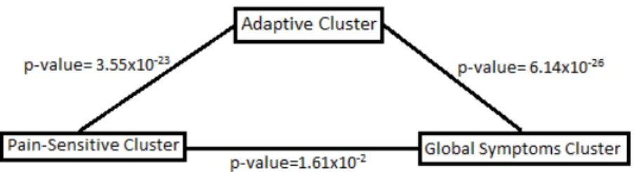
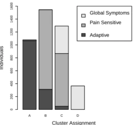
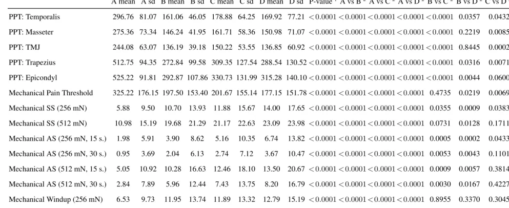
Full text
(2)(3)
(4)
(5)(6)
(7)
(8)
(9)
(10)
(11)
(12)
(13)
(14)
(15)
(16)
(17)
(18)
(19)
(20)
(21)
(22)
(23)
(24)
(25)
(26)
(27)
(28)
(29)
(30)
(31)
(32)
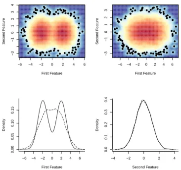
Figure

+7

Related documents
Keeping this tradition of epic poetry alive Pope has also used supernatural elements in “The Rape of the Lock”. Pope has
Volunteer ID Last Name First Name Spouse Last name Spouse First name Business Organization Business Position Business Address 1 Business Address 2 Business Address 3 Business
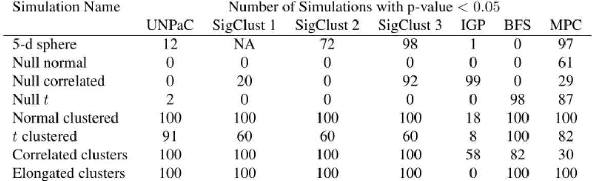
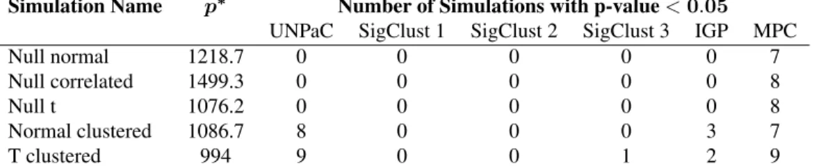
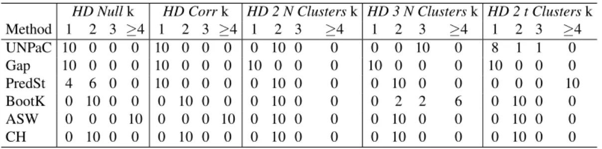
Table A-3.6 Marginal absolute effects of earthquake-related death of a family member on cumulative survival probability using outcome data partially imputed by risk score
Vehicle maintenance decisions are fully delegated to Municipal Fleet Maintenance Division whereas Ottawa Police Service Fleet and Technical Services concentrate mostly on
industrial action against the savage cuts in the education budget and the proposed changes to teachers’ pensions. Conference calls on Northern Committee to review and assess the
• If you have two or more job evaluation schemes covering all, or nearly all, your employees, you could estimate equal value by using the more generic job evaluation scheme to
9.3.1.3 The Bidder should propose a list of tools and test equipment (hardware and software) for TELCO PROV CO to acquire for daily O&M
Skills: Battle 3, Craft: Armorsmithing 4, Craft: Weaponsmithing 3, Defense 4, Engineering (Siege) 5, Etiquette 2, Iaijutsu 3, Investigation 2, Kenjutsu 3, Know the School:
