Cover Page
The handle http://hdl.handle.net/1887/25808 holds various files of this Leiden University
dissertation
Author
: Kloet, Frans van der
QUANTITATION IN UNTARGETED
MASS SPECTROMETRY-BASED
METABOLOMICS
PROEFSCHRIFT
Ter verkrijging van
de graad van Doctor aan de Universiteit Leiden, op gezag van Rector Magnificus prof. mr. C. J. J. M. Stolker,
volgens besluit van het College voor Promoties te verdedigen op woensdag 21 mei 2014
klokke 13:45 uur
door
Promotor: Prof. dr. Th. Hankemeier
Co-Promotor: dr. T.H. Reijmers
Overige leden: Prof. dr. M. Danhof
dr. W. Dunn
Prof. dr. J. van der Greef
Prof. dr. A.H.C. van Kampen
Prof. dr. A.K. Smilde
ISBN/EAN:978-90-74538-82-4
Cover by Anita van der Kloet
C O N T E N T S
1 i n t r o d u c t i o n 3
1.1 Mass Spectrometry 5
1.2 Quantification 7
1.3 Integration 8
1.4 Statistics and data analysis 10
1.5 Scope and outline of this thesis 11
2 a na ly t i c a l e r r o r r e d u c t i o n 13
2.1 Introduction 14
2.2 Workflow and methods 15
2.3 Batch calibration 19
2.4 Experimental 22
2.5 Conclusion 31
3 d i s c ov e r y o f e a r ly-s ta g e b i o m a r k e r s 33
3.1 Introduction 35
3.2 Experimental 36
3.3 Results and discussion 40
3.4 Conclusions 48
s3 s u p p l e m e n t t o d i s c ov e r y o f e a r ly-s ta g e b i o m a r k e r s 49
s3.1 Experimental 49
s3.2 Results 54
4 r a p i d m e ta b o l i c s c r e e n i n g.. 59
4.1 Abstract 59
4.2 Introduction 60
4.3 Materials and Methods 61
4.4 Results and Discussion 63
4.5 Concluding Remarks 70
s4 s u p p l e m e n t t o r a p i d m e ta b o l i c s c r e e n i n g.. 71
5 a n e w a p p r oa c h t o u n ta r g e t e d i n t e g r at i o n 73
5.1 Introduction 74
5.2 Workflow (and methods) 75
5.3 Experimental 80
5.4 Results and discussion 82
5.5 Discussion 86
5.6 Conclusions 87
s5 s u p p l e m e n t t o a n e w a p p r oa c h t o u n ta r g e t e d i n t e g r a
-t i o n 89
s5.1 Re-calibration of profile data 89
6 s u m m a r y a n d f u t u r e p e r s p e c t i v e s 95
7 b i b l i o g r a p h y 99
8 s a m e n vat t i n g 113
9 d a n k w o o r d 117
10 c u r r i c u l u m v i ta e 119
1
I N T R O D U C T I O N
In the Oxford Dictionary the metabolome is defined as: the total number
of metabolites (the small molecules that are intermediates or products as a
result of a metabolic reaction) present within anorganism,cellortissue. This definition covers the three key factors of metabolomics, the research field in-vestigating the composition, role and function of the metabolome [140]. In the
analysis of the definition of the metabolome we first identify the biological origin of the research field which can vary with regards to the type of biolog-ical question, and therewith connected, the type of samples that are analyzed. This can range from small individual cells to cells clusters to tissue slices to all sorts of biofluids like blood, urine or cerebrospinal fluid. Secondly, the term metabolite implies some form of identification of the chemical compounds be-ing studied. Popular profilbe-ing and identification methods range from Nuclear Magnetic Resonance (NMR) to Mass Spectrometry (MS). Recently in particu-lar fragmentation trees obtained with the MSn [61,106] approach are used to
assign identities to the data features obtained with MS-based profiling tech-niques. The total number refers to the number of identified (and unidentified) chemical (metabolic) features and their concentration levels that are detected with the same analytical techniques mentioned before.
To obtain biological interpretable results these three important types of infor-mation (identity, quantity, and biological relevance) on a metabolite (Figure1)
are equally important and interact strongly. For a good understanding of the biological context the identity of the metabolites must be known. Conversely, identification of metabolites can be greatly improved by including biological in-formation [58]. Furthermore proper (relative) quantification of the metabolites
in question [139, 91] is necessary for a better understanding and modeling of
Figure1: The three key factors of metabolomics: Biological relevance, Identity
and Quantity and their interactions.
The word metabolome itself is a construct of the words metabolism and genome [47] and hints to the hierarchy within cell biology: the metabolome is the
sult of a whole range of chemical and regulation processes that are the re-sult of the interaction of other biochemical organization levels such as the genome and their interaction with the environment. For example, changes in a cells physiological state as a result of gene deletion or overexpression are the complex result of processes at the transcriptome and the proteome and ultimately metabolome level[65, 126, 55]. For example, hard to detect
multi-factorial changes in the genome resulting in a disease may be easier detected by changes in the metabolite concentrations. This amplification of effects indi-cates the strength of metabolomics.
se-1.1 m a s s s p e c t r o m e t r y
lected part of cellular metabolic networks in a targeted manner, more recently tracer-based metabolomics has been developed as a new experimental data acquisition approach[77].
1.1 m a s s s p e c t r o m e t r y
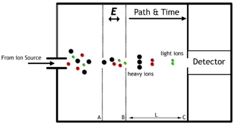
Hyphenated mass-spectrometry (GC, CE or LC-MS) has become the pre-dominant technology for determining metabolite abundances, mainly because of its sensitivity allowing the measurement of low abundant metabolites in small sample volumes. In Figure 2 the schematic of a time-of-flight (TOF)
mass spectrometer (MS) detector is shown. The analytes are ionized in the ion source and separated by the applied electric field E (between grid A and B) in which the ions are differentially accelerated depending on their mass and charge. The time it takes to reach the detector (from B to C (length L)) is char-acteristic for the mass/charge ratio of an ion. Ions with a lower mass (having the same charge) are accelerated more and reach the detector earlier due to
E = 12mv2 and consequentlym = 2E
v2 . vis the velocity i.e. the measured time (t) it takes for ions to travel the distance L.
Figure2: Schematic of a linear Time of Flight (TOF) mass spectrometer, heavier
ions (with same charge) travel proportionally slower than lighter ions in an electric field.
When all ions have reached the detector a mass spectrum can be generated (Figure 3). The intensity on the y- axis corresponds to the number of ions that
Figure3: A typical (part of a) mass spectrum.
A drawback in MS is that each metabolite has its own response factor, i.e. the signal depends on the number of molecules but also on the type of molecule. For example two metabolites showing up in a mass spectrum with each of its (e.g.) protonated molecule having an intensity of 106do not necessarily have
the same concentration when they are introduced into the MS. This depends on factors like solubility, ionizability, fragmentation, etc. [4], which are
differ-ent for the differdiffer-ent metabolites. In addition, mass-dependdiffer-ent discrimination can occur due to the mass spectrometer. Furthermore, the response factor for a certain metabolite is matrix dependent, i.e. dependent on the composition of the solvent (in which various compounds can be present) when introduced into the MS, and consequently can vary over different samples creating dif-ferences in measured responses for identical metabolite concentrations[6, 79].
With other words, in two different human plasma samples the same metabo-lite with the same concentration can have different responses. The complex interactions between analyte and the matrix, in which it was measured, can have a significant effect on the response in the MS; this is often referred to as ion suppression/enhancement effects. To compensate for these variations, correction of the response using internal standards is needed. These internal standards should have the same chemical behavior as the analyte but should be detected separately from the analyte of interest. The best internal stan-dard for a certain metabolite is the stable isotopically-labeled (D,13C or 15N) metabolite itself[78]. Once added to the sample the response of the
(isotopi-cally labeled) internal standard can be used for correction of different kinds of chemical and instrumental variations like sample treatment differences, pipet-ting errors, storage effects, ion suppression etc.. The ratio between the peak intensities of the analyte and internal standard gives an indication of the rela-tive (to the selected internal standard) concentration of the analyte. Absolute quantification of the actual concentration levels (e.g. µmol
µl ,
g
kgetc.) in all samples
1.2 q ua n t i f i c at i o n
liquid chromatography (LC) or capillary electrophoresis (CE). In addition to an improved separation of analytes of interest, possible matrix effects and con-sequently ion suppression effects may be significantly reduced this way.
1.2 q ua n t i f i c at i o n
To get reliable quantitation (preferably absolute) the observed differences between the different analyzed samples should not be hampered by analytical variation and should be attributed only to real biological differences of interest. Consequently any further (data) analysis then solely can focus on interpreting these differences. The quantifiable response for a metabolite is the product of its concentration and a metabolite specific response factor. The response factor however, is affected by matrix effects which necessarily need to be minimized. The common ways to characterize these matrix effects are either by post col-umn infusion methods or post-extraction spiking methods[23,87]. Because the
first method only characterizes the matrix effects qualitatively, the quantitative assessment using the second method is more common. With both methods however, the characterisation is biased towards a set of known metabolites only. In metabolomics where typically hundreds to thousands of (also uniden-tified) metabolites are measured, it is very uncommon to measure (internal) standards for each of these metabolites. This would be very laborious and thus expensive. In addition, it is not known a priori, which metabolites are of interest for the study at hand. As a consequence often platforms are used that cover a wide range of metabolites whose identity is not known in advance (so called untargeted platforms). In these cases usually at least one internal stan-dard per class of metabolites is included to enable relative quantitation (e.g. on lipid per lipid class in lipidomics[53]).
The choice of a proper internal standard influences the estimated (relative) concentration of the compounds in question. Figure4a shows the peak areas
of L-Leucine and two internal standards that were added in replicated (GC-MS) measurements[8, 48] of over 100 identical reference samples (technical
replicates [32], i.e. the complete analytical process rather than repeat injections
of the same sample). Because the measurements concern the same sample, the ratio between the analyte and the internal standard (IS) should remain constant. The ratios of L-Leucine with the internal standards are plotted in Figure 4b. It is clear that correction with Leucine-D3 generates an almost
constant value. However, it is also obvious that correction with a less suitable internal standard (in this case Phenylalanine-D5) can have a dramatic effect on
Figure4: (a) The peak areas of L-Leucine and2internal standards for a series
repeated measurements (112technical replicates) of a QC sample. (b)
The ratio plot of L-Leucine with each of the two internal standards.
If the ideal internal standard is not available or used, there are four levels of correction to consider to estimate the relative concentration: between ana-lytes within one sample, between anaana-lytes over samples measured within one batch and, when many samples need to be measured that cannot be processed within one batch, between analytical batches of samples, and finally, when there is also a substantial time difference between measurements of sample sets, between studies correction. The common factor in all of these four levels is (acquisition) time and in specific all kinds of instrumental and environmen-tal variations like matrix differences, sample degradation, different apparatus but also preprocessing/integration variation that have changed in this time. The challenge in metabolomics is to minimize these variations for as many as possible different metabolites. It is at this stage that metabolomics greatly ben-efits from statistics (e.g. experimental design [67], data analysis) but of course
also from improved analytical sample preparation and analysis methods. With regards to analytical methods, one could think of using a different analytical setup (e.g. post-column infusion techniques [23]) that would quantify
suppres-sion effects for a whole range of metabolites but also other optimizations of experimental conditions like concentration levels of the added internal stan-dard [104, 105, 10] can be considered. Statistically, a (mathematical) solution
could be to construct virtual internal standards based on a (multivariate/lin-ear) combination of internal standards to normalize the responses of unknown compounds. Finally, to improve comparison over analytical batches of sam-ples and between studies appropriate reference samsam-ples could be used[54].
The choice which samples to use as a reference would be a clear result of the combined efforts in analytics and statistics.
1.3 i n t e g r at i o n
Even if all analytical and instrumental settings are optimized, one issue in analyzing MS data that is often left untouched is the integration step itself. The principle to translate the area under the (unimodal and non-overlapping) curves to areas belonging to2 different components as shown in Figure5a is
1.3 i n t e g r at i o n
Figure5: (a) Unimodal extracted ion chromatogram (EIC). (b) Bimodal EIC,
(where) should the peaks be separated?
In case of bimodality or multi-modality curves (e.g. due to not fully separated isomers) things get more complicated and arbitrary decisions have to be made (Figure 5b); solutions are to calculate the sum of the total peak are under the
curve, split them in the middle or try to fit the signal by (two or more) sep-arate peaks (i.e. by deconvoluting them). Once a choice has been made the software has to be parameterized accordingly. Different (MS) vendors provide own software packages for integration and it is at this point where the differ-ent software packages show differdiffer-ent outcomes for almost iddiffer-entical cases as depicted in Figure6(a and b).
Figure6: The unexpected behavior with automated integration software. (a)
The peak is split in three separate peaks. (b) The two right peaks are combined.
In Figure6 the same cases of multi-modal peaks are split in different ways
manual curation procedures as in targeted data processing is hardly feasible.
Despite the limited number of compounds reported and expensive manual data curation, targeted approaches are widely used. Obvious reasons are that the targeted metabolites/compounds are known which is very important for the data interpretation, and the possibility to quantify them (using internal standards and reference compounds) often with better precision and accuracy then in untargeted modes. To a large extent this is also due to the lack of appropriate software that would enable untargeted extraction and integration without introducing artifacts and errors. As a result, integration is often lim-ited to a set of known metabolites (targets) only and in most cases vendor software is used for such targeted data processing.
1.4 s tat i s t i c s a n d d ata a na ly s i s
In metabolomics statistics are applied throughout the whole process of an-alyzing samples, from method development to data analysis. Experimental designs are applied to setup a study in such a way to minimize the number of experiments while retaining the maximum amount of information[67].
Re-peated measurements of samples are used to statistically indicate whether or not the analytical platform functions within specification[37]. To this extent,
often, for each specific metabolomics study, a pooled sample (a so-called Qual-ity Control sample) from all samples of that study is created and repeatedly measured. As mentioned earlier, correction steps are necessary to compare metabolites between and over samples. Depending on the type of sample, the way it was measured etc., a whole range of statistically data pretreatment (normalization) methods are offered to improve ultimately the biological inter-pretation of the data[127]. Actually most, if not all, statistics (in metabolomics)
are performed to remove/indicate analytical variation in metabolites (features) that are measured. Those features that do not meet the pre-defined criteria are usually removed from the dataset and further data analysis/interpretation is continued with a smaller set of reliable metabolites. This removal does not necessarily improve biological interpretation but the complexity of follow-up (data) analysis can be reduced considerably.
In univariate statistics the focus is on one variable at a time and the results are relatively easy to interpret from a statistical point of view (e.g. the effect of the variable is significant or not using T-tests[89]). As a consequence
univari-ate statistics methods -are widely accepted, especially in clinical settings[147, 100]. Because changes in biological samples are often multifactorial[147, 100],
1.5 s c o p e a n d o u t l i n e o f t h i s t h e s i s
analysis (PLS-DA)[142] are commonly used to relate these differences to
spe-cific metabolites. Using statistical modeling of properly quantified metabolites, (multivariate) metabolic networks can even be inferred[44]. Because of the
lim-ited number of samples in comparison to the huge amount of variables (e.g. metabolites) that are measured, multivariate models easily lead to overfitted results (i.e. perfect fits are found, but the predictive power of the model is limited). The results are hugely aided by variable selection methods to se-lect the important from the less important variables and cross-validation and permutation[142] procedures to prevent this overfitting when building
predic-tive multivariate models.
1.5 s c o p e a n d o u t l i n e o f t h i s t h e s i s
In the previous paragraphs some typical challenges were discussed that re-searchers are faced with when handling data from metabolomics studies using untargeted mass spectrometry based data. The aim of this thesis was to de-velop concepts and methods to extract qualitative and quantitative information about metabolites from untargeted mass spectrometric data. For this, different methods were developed to obtain quantitative metabolite data in large stud-ies using GC-MS, LC-high resolution MS (HR-MS) and direct infusion high resolution mass spectrometry. The different methods address different parts in the metabolomics workflow, i.e. data -acquisition, data pre-processing up to data-analysis.
As the performance of analytical systems can vary, different methods of normalization to improve quantification for known and unknown compounds were developed. In Chapter2 it is demonstrated that for (relative) quantifica-tion of metabolites in GC-MS metabolomics studies, in the absence of matched stable isotopes, per metabolite normalization based on a single internal stan-dard is not enough to correct for analytical batch-to-batch differences. This is especially troublesome in large scale metabolomics studies where many samples need to be measured and consequently many analytical batches are needed. Furthermore, even within a single analytical batch a clear trend in the response for specific metabolites was observed. A statistical procedure based on repetitive measurements of identical samples (i.e. technical replicates) is suggested that corrects for these batch-to-batch differences even for metabo-lites without a proper internal standard.
In Chapter 4 a method has been developed and demonstrated for the pro-cessing of another type of very complex metabolomics data, i.e. metabolomics data obtained by direct infusion mass spectrometry. It was demonstrated that with the preprocessing method that was developed, biological relevant results, i.e. the characterization of different development stages of zebrafish embryos, could be extracted from these very complex metabolomics data. Feature iden-tification was solely based on accurate mass and therefore the samples were recorded with a very high mass resolution. The method developed was based on the binning tools developed for LC-MS (Chapter5) by aligning the masses
over samples which enabled further automated data analysis. Internal stan-dard correction for the unknown features was based on the same strategy as described in Chapter 2. In the absence of quality control samples however,
the relative standard deviation (RSD) was calculated using replicated measure-ments.
The integration problems that were observed during pre-processing of un-targeted LC-MS data from earlier experiments (including those reported in Chapter3), led to the awareness of the lack of good software to integrate peaks
2
A N A LY T I C A L E R R O R R E D U C T I O N U S I N G S I N G L E P O I N T C A L I B R AT I O N F O R A C C U R AT E A N D P R E C I S E
M E TA B O L O M I C P H E N O T Y P I N G
a b s t r a c t
Analytical errors caused by suboptimal performance of the chosen platform for a number of metabolites and instrumental drift are a major issue in large scale metabolomics studies. Especially for MS-based methods, which are gain-ing common ground within metabolomics, it is difficult to control the analyti-cal data quality without the availability of suitable labeled internal standards and calibration standards even within one laboratory. In this paper we suggest a workflow for significant reduction of the analytical error using pooled cali-bration samples and multiple internal standard strategy. Between and within batch calibration techniques are applied and the analytical error is reduced sig-nificantly (increase of 25% of peaks with RSD lower than20%) and does not
hamper or interfere with statistical analysis of the final data.
2.1 i n t r o d u c t i o n
Recently there has been an explosion of analytical methods developed and applied in different metabolomics related research areas, such as nutrition research[90, 13, 135, 35] , drug discovery[63], optimization of fermentation
processes [132, 131] and for breeding [24] of plants. In all these applications
it is important to be able to understand and control factors that contribute to errors in the data and result in poor data quality. The total variation in a dataset is a function of different sources of variation[128]. The biological
vari-ation is present by design of the study and selection criteria of the subjects. In some cases, additional ’biological’ variation can be introduced by differences in sample collection and sample storage [111,25] Samples drawn from
biolog-ical systems such as a microbiologbiolog-ical fermentation or from body fluids like blood or urine are highly susceptible to changes due to biological reactions that take place, especially when the environment of the sample changes. It is therefore essential that changes in metabolites are minimized during sampling and sample preparation [131] in order to obtain a snap-shot representation of
the biological system at the time of sampling. From an analytical point of view the data is of a much higher quality than years ago thanks to the efforts of instrument vendors to obtain more reproducible data, but it is still not enough. The analytical errors should be controlled as much as possible and reduced to a minimum and should not be confused with biological differences within the studied system.
2.1.1 Sources of analytical variation
A large part of the analytical variation is caused by suboptimal performance of the chosen platform for (sub-)sets of metabolites and instrumental drift. The ability of a method to detect a specific metabolite (i.e. its performance) is a complex interplay of its physical and chemical properties and is also partially dependent on the sample composition (matrix, e.g. ion suppression in MS based systems [11]) and in many cases on its concentration. Analytical
2.2 w o r k f l o w a n d m e t h o d s
where hundreds of (also unidentified) metabolites are measured it is very un-common to measure calibration standards for each of these metabolites. This would be very laborious and thus expensive, but equally important is the fact that beforehand it is not always clear which metabolite is of interest for the study at hand. In order to assess the data quality of all of these metabolites the use of pooled study (QC) samples has been described recently in the literature [28, 37]. In this approach pooled samples are analyzed regularly in between
the individual study samples, several times within each batch. As a pooled study sample reflects the average metabolite concentrations within a study, this sample contains the same compounds (e.g. metabolites) as all the other samples. The performance of the analytical platform for all the compounds can be assessed by calculating the relative standard deviation (population standard deviation divided by the population mean) in these pooled samples [129, 28].
Various approaches to detect artifacts are described in Burton et al.[18]. Most
of them however depend on visual inspection. Descriptions of data quality improvements are quite scarce. This paper describes a workflow for signifi-cant reduction of the analytical error using these pooled QC samples. Based on a multiple internal standard strategy and moreover between and within batch calibration techniques the analytical error is reduced significantly and will thus not hamper statistical analysis of the final data. Although this paper focuses on GC/LC-MS measurements and peak areas, it should be noted that the solution presented here is generic.
2.2 w o r k f l o w a n d m e t h o d s
For an effective removal of different sources of analytical variation the pre-processing steps should follow a specific sequence. The first step is the data normalization using an internal standard. This step reduces the differences in sample extraction (which can be caused by slight differences in the composi-tion of the samples) and also differences in the volumes injected. Especially the latter issue is of importance when injecting such low volumes as 1-2 µl.
The second step is the removal of between-batch and within-batches batch offsets and drifts. This step can only be omitted if each metabolite has a struc-tural analogue IS that corrects for all offsets and drifts, which is not the case in metabolomics analysis. The final steps consist of the combination of data from replicate sample analysis and removal of noise [13] and biomass
correc-tion [141]. The biomass correction neutralizes differences in response due to
fully automated environment.
2.2.1 Used symbols and terminology
Terminology
Internal standard: There are several definitions of internal standards and sur-rogates in the literature describing analytical methods. In this publication in-ternal standard is a compound added to the sample before a critical step in the analysis. Depending on the method, the internal standard can be added before or during the extraction of the sample, derivatisation steps, etc.. An internal standard is not necessarily an isotope labeled version of an analyte but can also be structurally related to one or more analytes but not naturally occurring in the samples of interest. If a method covers analytes from different compound classes, multiple internal standards preferably covering all classes should be used.
Batch: a group of samples that has been extracted, derivatised (if applicable) and analysed together at the same time and using the same chemicals, same storage conditions.
QC sample: sample prepared by pooling aliquots of individual study samples, either all or a subset representative for the study. The QC sample has (should have) an identical or a very similar (bio) chemical diversity as the study sam-ples. If insufficient sample volumes are available (e.g. rodent studies), samples collected outside the study but from a similar origin can be used. The QC sam-ples are evenly distributed over all the batches and are extracted, derivatised (if applicable) and analysed at the same time as the individual study samples as part of the total sequence order.
QC calibration sample: sample chemically identical to the QC sample (from the same pool), prepared in the same way as QC samples. QC calibration samples are used for external calibration.
QC validation sample: sample chemically identical to the QC sample (from the same pool), prepared in the same way as QC samples. QC validation samples are solely used to monitor the result of all the data pre-processing steps and the quality of the full method. They are not used for external calibration.
Peak: For the purpose of this publication we use a broader definition of peak. A peak can be a single feature (intensity of a mass/ion or a different signal at a retention time or shift) or can be a sum of features (summed intensity of several ions at the same retention time). In our examples one peak represents one compound or metabolite detected in the data.
2.2 w o r k f l o w a n d m e t h o d s
Assumptions
The method described in the procedure below focusses on peaks. The study samples vary in concentration for several peaks. For the purpose of this publi-cation and all the procedures described here, we assume that response factors and the analytical performance of the internal standards and individual ana-lytes are not influenced by the sample differences. In other words, the analyt-ical performance of the method for all the individual analytes observed in the pooled QC sample will be the same in all other individual study samples.
Used symbols
i index number for samples
p Chromatographic peak (chemical component)
Cp,i Concentration of peakpfor samplei
Fp Response factor for peakp
Fp(t) Response factor for peakpat time pointt Fp,i Response factor for peakpfor samplei
Gp,i Transformed form ofFp,i after internal standard correction Xp,i Measured response of peakpfor samplei
Xis,i Measured response of internal standard peakisfor samplei X0p,i Relative response after internal standard calibration of peakp X0qc,p,b Relative response after internal standard calibration of peak p
for QC calibration samples in batchb
X00p,i Relative response after internal standard calibration and batch calibration of peakpfor samplei
Ap,b Average amplification relative response factor for peak p in
batchb
cfp,b Calibration factor for peakpin batchb
αp,b,qc Slope for linear estimate of QC calibration values for peakpin
batchb
βp,b,qc Intercept for linear estimate of QC calibration values for peak pin batchb
Gp,b,i Linear estimate of QC calibration values for peakpfor sample
iin batch b
Z Smoothed estimate of QC calibration values for a single peak
in a single batch
2.2.2 Internal Standard normalization
When focussing on MS analysis, it is generally difficult to model the ex-traction (derivatisation), MS ionisation and fragmentation variability of a com-pound by the behaviour of an internal standard with very different physical-chemical properties. This is especially the case when compound and reference belong to chemically different classes (e.g. glucose-d7is a good representative
chem-ical similarity (e.g. glucose-d7 is also expected to be a good internal standard
for fructose and other hexoses). One could argue which internal standards, if more are included, should be used to adequately correct the errors in the mea-sured responses of the individual metabolites. Sysi-Aho et al.[122] suggest
selecting the best internal standard based on similarity between the distribu-tions of the available internal standards and the compounds that are measured. Measurements that are performed at a later stage are then corrected using the preferred internal standard. This way however, real-time analytical variation is not included in the internal standard selection process which may result in sub-optimal error correction. We suggest using analyte responses in quality control (QC) samples, regularly analyzed in between the study samples, as means to find the best internal standard. Using the relative standard deviations (RSDs) of the analyte response in the QC samples to quantify the amount of analytical variation, the best internal standard is the one that gives a minimum relative standard deviation.
In general, the response of a detector for a peakpcan be defined as a product of its concentrationCpand a response factor Fp specific to this compound. For
sampleithe measured response Xp,i is defined as shown in Equation1.
Xp,i =Cp,i·Fp (1)
In an ideal situation Fp is constant and therefore measurements with a
con-stant Cp,i have identical responses. The RSD of QC samples for each peak
would then be zero.
Internal standards are routinely used to correct systematic errors in the mea-sured response by transforming the meamea-sured response Xp,i into a relative
response X0p,i using the measured response Xis of the internal standard is as
denoted in Equation2.
X0p,i = Xp,i
Xis,i
(2)
This transformation and its error correcting effect is based on the assump-tion that for a perfect internal standard the sensitivity of the instrument for compound pis directly related to the sensitivity of the instrument for internal standard IS. In case of a non ideal standard, the corrective effect is not pre-dictable. It may range from almost as good as the ideal internal standard to an actual increase of the error. In typical metabolomics methods the correc-tive effect of internal standards is highly variable because the number and the chemical diversity of the analytes exceed that of the internal standards (only a few metabolites form a perfect pair with a certain internal standard in a typical dataset).
The RSD for the QC samples is calculated using Equation 3, in which the
standard deviation (σX0
p,qc) (after internal standard correction) is divided by the
average (<>) relative response after internal standard correction(<X0p,qc>)
RSDp,qc=
σX0 p,qc <X0
p,qc >
(3)
The best internal standard is the one that results in a minimal RSD. This
2.3 b at c h c a l i b r at i o n
2.3 b at c h c a l i b r at i o n
Adjustments of the analytical instrument (e.g. maintenance, cleaning, tuning etc.) between batches of samples can be the cause of analytical errors that can-not be corrected for using solely internal standard calibration. This behaviour exerts itself in different response factors between and even within batches. We suggest that QC samples describe this type of analytical variation adequately and as a result, QC samples can be used as a means to correct for it. This type of correction is referred to as batch calibration.
2.3.1 Mean and median correction (between-batch)
Assuming that the measurement errors in a single batch are randomly dis-tributed, then different batches can be compared and corrected using the aver-age or median value of the QC samples in a batch. The averaver-age amplification relative response factor per peak per batch (Ap,b) can be written as the average
(¡ ¿) of the responses after internal standard correction of the QC samples per batch (Equation4).
Ap,b=<Xp0,qc,b> (4)
The between batch calibration concerns the adjustment of the amplification factorcfp,bper peak with respect to a reference batch (in Equation 5batch1is
taken as reference).
cfp,b= Ap,1
Ap,b
(5)
The error between measurements in a single batch is assumed to be a ho-moscedastic and random effect and therefore the same offset correction factors obtained from the QC samples can be transferred to the samples that are mea-sured in between the different QC samples per batch.
X00p,b,i =cfp,b·X0p,b,i (6)
As an alternative, the median can be used for determining the batch correc-tion factor (in Equacorrec-tion 4) instead of the average. This has advantages over
the mean in being a more robust measure. However, most parametric (statisti-cal) tests, that for example facilitate outlier detection, are focussed on averages which makes the use of the average advantageous.
2.3.2 Linear regression (within-batch)
In many cases the response of the QC samples is not randomly distributed within a sequence of measurements and a notable drift can exist. In such cases the mean or median correction method will quite adequately correct for differences between batches but poorly for samples within a batch. If it is assumed that the behaviour between two consecutive QC samples is linear it can be modelled using first order regression. Mathematically, Equation1still
at which the sample was measured within a sequence. Equation 1 has to be
rewritten to Equation7.
Xp,i(t) =Cp,i(t)·Fp(t) (7)
Assuming that the analysis time of each sample is the same, time is equiva-lent to injection order and Equation7reduces to Equation8.
Xp,i =Cp,i·Fp,i (8)
After internal standard normalization has been performed the definition of QC calibrated data follows Equation9, in whichGp,iis the transformed form of
Fp,i after internal standard correction. The data are not calibrated for between batch differences. This is done as the final step.
X00p,i =cfp,i·X0p,i = X0p,i· 1
Gp,i
(9)
Because for each batch the correction factor is different, Equation9translates
into Equation10.
X00p,b,i =cfp,b,i·X0p,b,i =X0p,b,i· 1
Gp,b,i
(10)
The estimated trend of the (relative) response for the QC samples per peak within a batch can be written as a function of injection order that is adjusted for slopeβ, and an interceptα(Equation11).
X0p,b,qc =βp,b,qc·ib,qc+αp,b,qc (11)
In case of a first order regression the factorsαandβcan be calculated using regular linear regression. Although higher order regression methods can be applied they heavily depend on the number of QC samples that are measured and are more sensitive to outliers. Using the regression coefficients from Equa-tion11an estimate of the QC response can be calculated at each injection point
iwithin a batch. In order to make a good estimation the QC samples should be distributed evenly within the measurements in a batch to ensure a good representation of the total drift during a batch and measured at each start and end of a batch to prevent extrapolation (errors).
Gp,b,i =βp,b,qc·ib+αp,b,qc (12)
Using this estimated trend, the relative response after internal standard cali-bration, per batch, is divided by this trend (Equation13)
X00p,b,i =cfp,b,i·X0p,b,i = X
0
p,b,i Gp,b,i ≡ X
00
p,i (13)
2.3.3 Linear smoother
2.3 b at c h c a l i b r at i o n
1 2 3 4 5 6 7 8 9 10
0 10 20 30 40 50 60 70 80 90 100
injection order
response (y)
penalized least squares for f(x)=x2. λ=0, 10 and 105
original y λ=0 λ=10 λ=105
Figure1: The effect of different values ofλ on the smoothed estimateZ of an
arbitrary trend exhibited by QC samples (e.g. f(x) = x2). The black stippled line, whereλ =105 is used, is a horizontal line through the mean value of the QC samples. The blue dotted line, λ = 10, is a smoothed line that follows the general trend of the QC samples. The green line,λ=0, follows the exact pattern of the QC samples.
variation (noisy data) for a significant linear trend. Linear correction would still improve the overall quality but could also introduce new analytical vari-ation. In such cases the drift would best be described by a smoothed trend. Eilers[29] has shown that discrete penalized least squares can be used to
esti-mate a smoothed trend. λis the smoothing parameter where a largerλresults in a smoother estimate of the regression line Z. For really large values of λ,
Z will result in a horizontal line (Figure 1, the black stippled line). This is
a favourable characteristic because in cases of these large λs it is the only as-sumption that can be made (i.e. there’s no overall linear relation between the QC samples). For small values ofλhowever, Zfollows the trend exhibited by the QC samples (Figure1, the blue dotted line). When no penalty is imposed
the smoothed estimate Zfollows the exact pattern of the QC samples (Figure
1the green line).
To find an appropriate value for the penalty,λphas been made proportional
to the residual error of the linear estimate (Gp,b) and the actual QC sample
results in a smoothed estimate of the trend between consecutive QC samples. The final QC trend is removed via
X00p,b,i = X
0
p,b,i
Z0p,b,i (14)
Finally the calibrated response is calibrated for between batch differences using the math as described in Equations 4 through6. In this case however,
X0p,i is substitued byX00p,i.
2.4 e x p e r i m e n ta l
2.4.1 Data sets
To demonstrate the use of QC samples for the determination of the best internal standard and batch (between and within) calibration techniques two different datasets were used.
Data processing was performed using the MSD ChemStation E02.00.493
(Ag-ilent technologies, Santa Clara, CA, USA). Based on many previous studies a target table is pre-defined containing matrix and study specific (metabolites with known and unknown identities). Each peak is characterized by its reten-tion time and selected specific m/z value. For each study an update of the retention times (and in limited cases m/z) values is prepared. A limited num-ber of selected chromatograms are compared to a chromatogram of a reference sample (sample that is analysed in each study). Peaks that have not been ob-served previously are added to the target table. Artefacts of the method are removed from the data as well as (multiple) entries for a single (identified) metabolite caused by different derivatization products of which the perfor-mance is known to be irregular. For plasma, typically120-200metabolites are
reported. Even though this procedure is quite time-consuming, we believe it gives more reliable data than peak picking procedures or most deconvolution procedures with less missing values and less peaks. During acquisition of both datasets the following compounds were used as internal standards: Alanine d4 (ALA-D4), Cholic acid d4 (CA-D4), Leucine d3 (LEU-D3), Phenylalanine
d5 (PHE-D5), Glutamic acid d3 (GLU-D3), Dicyclohexylphtalate (DCHP),
Di-fluorobiphenyl (DFB), Trifluoroacetylantracene (TFAA). All compounds were purchased from Sigma (Zwijndrecht, the Netherlands).
Example metabolomics study1
A nutritional intervention study that involved 36 volunteers. Volunteers
were divided into 4 groups and received 4 different treatments: A, B, C and
D, including placebo. A cross-over design was used in this study, with each group receiving each of the treatments, in a randomized order [7]. At the
end of each treatment period each subject received an oral lipid challenge test, after which several blood samples were collected. Plasma samples collected within this study were analysed using different metabolomic platforms includ-ing the GC-MS method as described by Koek et al.[72] From the challenge
2.4 e x p e r i m e n ta l
and this data is used for the application demonstration of the developed work-flow and methods. Plasma samples (100µl) were extracted with methanol and
after evaporation the metabolites were derivatized (oximation and silylation).
8 different internal standards were added to the samples before the different
sample preparation steps. The number of individual study samples analysed by GC-MS was504. The samples were analysed in18batches, each batch
con-tained 28 study samples (all timepoints from two subjects, randomized per
subject) and3pooled QC samples. Each study sample was injected once; each
QC sample was injected twice per batch. The QC injections were distributed evenly in the batch: at the start of the batch, after approximately every6
sam-ples and at the end of each batch. Besides these QC samsam-ples, additional QC validation samples were included. Each batch contained1QC validation
sam-ple. At the end of the analysis, a 19th batch was included, which contained
a real replicate analysis of the complete time profile of two selected subjects. For this purpose a separate aliquot of the samples was extracted, derivatised and analysed. Data processing was performed as described above. 145peaks
(excluding internal standards) were reported.
Example metabolomics study2
An inflammation modulation study with placebo and diclofenac was per-formed in parallel [144]. Each group had 10 volunteers. 19 volunteers
com-pleted the treatment. Blood samples were taken after an overnight fast on days0,2,4,7and9. Subjects underwent an oral glucose tolerance test (OGTT)
on day 0 and day 9 of the study. Blood samples were taken just before (0
minutes) and15, 30, 45, 60, 90, 120and180 minutes after the administration
of the glucose solution (75 grams). The samples taken at day9were analysed
using the same analytical methods described for example study1. The
num-ber of individual study samples analysed by GC-MS was 361 (19 volunteers, 19timepoints per volunteer), each sample was analysed twice, resulting in722
sample injections. The samples were analysed in 26 batches, each batch
con-tained 35 injections including QC samples. Batch 1 started with all samples
of one of the subjects, timepoints randomized, followed by the randomized replicate measurements of the same subject until the maximum of29 (sample)
injections was reached. The next batch started with the remaining (replicate) samples of the previous subject followed by the, timepoint randomized, full set of samples of the next subject etc. In this way for each subject at least one replicate of the full time profile was analysed within one batch. The QC injections were distributed evenly in the batch: at the start of the batch, after approximately every 6 sample injections and at the end of each batch. No
additional QC validation samples were measured. To assess the effect of the different preprocessing steps the replicated measurements were used. Data processing was performed as described above. 137peaks (excluding internal
standards) were reported.
Data extraction
Both example studies were processed using a target approach. The target table was adjusted 3 times for retention time shifts caused by shortening the
Data processing
Prototyping of the correction methods was executed in Matlab version2007b[50].
The final implementation of the software was done in SAS version9.1.3[52] as
stored procedures complementary to a data warehouse (SAS) in which the study data were captured.
2.4.2 Results and discussion
Internal Standard normalization
The number of internal standards is dependent on the analytical method
with a minimum of 1 and no maximum. To mimic the behaviour of the
an-alytes structure analogues and stable isotope labelled compounds were used added as internal standards. In our example study we used 8 internal
stan-dards and applied our selection method to select the most suitable one. Table
1 shows the results of the selection method on theRSD values of the QC
cal-ibration samples. That the RSD indeed seems to be functioning as a good criterion for the selection of the best internal standard is shown in Table 2 in
which examples are shown of the internal standard that was selected as best for a number of identified metabolites in metabolomics study 1. In all cases
where an analyte had an own deuterated internal standard, this standard was selected, as it also gives the lowestRSDin the QC validation samples. For com-pounds with no deuterated analogue a structurally related IS was selected, e.g. LEU-D3 was selected for the corrections of both leucine and isoleucine, for
alanine, ALA-D4 is selected. For some aminoacids within this study, the the
deuterated analogue gives a slightly higher RSD than a different deuterated IS ( 8% vs5%). Within this study this is the case for glutamate, for this
com-pound PHE-D5is selected as the IS giving the lowestRSDin the QC validation
samples. Within this study, not all the reported metabolites have a suitable IS structurally. For example the detected fatty acids are less volatile and elute later in the chromatogram. For these matabolites the described procedure chooses apolar and/or late eluting internal standards such as DFB or DCHP as the most suitable. It should be noted that each metabolite might have sev-eral suitable IS within the approach giving similarRSD values. Therefore the chosen IS can differ from study to study, depending on the dataset.
RSD Corrected for 1IS (DCHP) corrected for best IS
0%-10% 26% 58%
10%-20% 32% 24%
20%-30% 27% 10%
>30% 16% 8%
Table 1: Frequency distribution ofRSDvalues of QC calibration samples from
the first example study. The effect of the ’best’ internal standard clearly translates into more peaks with lower RSDvalues.
Each of the peaks was assigned a best internal standard (1 out of 8) using
the criterion as described in Equation 3. After the normalization step with
cluster-2.4 e x p e r i m e n ta l
−12 −10 −8 −6 −4 −2 0 2 4 6 8
−15 −10 −5 0 5 10 15
Scores on PC 1 (17.31%)
Sco
re
s
o
n
PC
2
(1
3
.7
9
%
)
Samples/Scores Plot
Figure2: PCA score plot of QC calibration samples from the first example
study after internal standard normalization. Different colours refer to the different batches. The data are autoscaled. Two clusters are visible; one before cleaning the MS source (left) and one after the cleaning procedure (right).
ing of the different QC samples per batch. Furthermore, the plot shows that there’s a significant difference between two clusters of batches. Investigation reveals that the group on the left hand side are batches1-9whilst the
remain-ing batches10-19are plotted on the right hand side; it coincides with the fact
that the MS source was cleaned after the9th batch. This behaviour emphasizes
that QC samples (indeed) characterize the systems state (or can be used to do so). It also leads to the conclusion that remaining variation due to between-batch and/or within-between-batch differences is insufficiently corrected for using the normalization procedure with internal standards.
Metabolite IS selected as best
Alanine ALA-D4
Leucine LEU-D3
Isoleucine LEU-D3
Glutamic acid PHE-D5
C16:1Fatty acid DFB
C16:0Fatty acid DCHP
C17:0Fatty acid DCHP
Table 2: Examples of the selected best internal standard for a selection of
Batch calibration
Figure 3a shows a part of a time order profile plot of a specific metabolite
from the second example study. The real samples are represented by the blue triangles and the QC samples by the red crosses, the green lines represent the smoothed estimate for the trend exhibited by the QC samples. Each verti-cal dashed line represents the start of a new batch. The figure clearly shows the effect of analytical errors that are introduced during measurements. Even though the data was corrected for the best internal standard, for some metabo-lites such as this example, large between-batch and within-batch differences still exist for the QC samples. The study was not set up for quantification purposes but it is apparent that for any further (statistical) analysis this type of error should be removed. In order to do so, a smoothed trend, per batch, was fitted through the QC samples. Figure 3b shows the results of the same
metabolite after the batch calibration step. The RSD value of this metabolite for the QC samples dropped from 13.7% after internal standard correction to 2.1% after the additional batch correction step. The QC samples follow an
2.4 e x p e r i m e n ta l
770 780 790 800 810 820 830 840
3 3.5 4 4.5 5 5.5 6 6.5
x 105
injection order IS co rre ct e d re sp o n se a
770 780 790 800 810 820 830 840
0.5 0.6 0.7 0.8 0.9 1 1.1 1.2 1.3 1.4 1.5 injection order IS a n d Q C co rre ct e d re sp o n se b
Figure3: A part of the time order plot of a specific metabolite from the second
Validating the results
The availability of QC calibration, QC validation samples and replicated sample measurements allow for a triple validation check. The performance statistics used are as follows:
1. Improvement ofRSD in the QC calibration samples
2. Improvement ofRSD in the (independent) QC validation samples
3. Improvement of differences between samples with different composition
(representative replicates)
The effect induced by the different calibration steps on the RSDvalue of the QC validation samples from the first example study is shown in Table 3. The
table shows the distribution of the number of metabolites when theRSDrange is divided into4 classes. For replicated measurements the results are shown
in Table 4. The results in Table 3 and Table 4 are comparable, the removal
of between and within batch differences using the real-time variation informa-tion embedded within pooled QC samples shows a significant impromevent in observedRSDvalues.
RSD Raw data IS calibrated IS + batch calibrated
0%-10% 12% 58% 81%
10%-20% 59% 24% 16%
20%-30% 16% 10% 3%
>30% 13% 8% 0%
Table 3: Frequency distribution of RSD values of the QC validation samples
from the first example study. The IS normalization and batch cali-bration steps clearly have a favourable effect on the RSD frequency distribution of these samples.
RSD Raw data IS calibrated IS + batch calibrated
0%-10% 49% 53% 72%
10%-20% 36% 32% 21%
20%-30% 8% 8% 7%
>30% 8% 7% 1%
Table 4: Frequency distribution ofRSD values of duplicated measurements of
real samples from the second example study. The calibration steps show the same positive effect on the frequency distribution of ’RSD’s of these replicate measurements as the QC validation samples.
Visualizing information potential
2.4 e x p e r i m e n ta l
depicting the improved data quality obtained with the QC calibration method. An example for GC-MS data from the second example study is shown in an Information Density plot (ID plot) (Figure 4 a and b). The x-axis shows the
RSD, and the y-axis shows the correlation between replicates. The correlation is both a measure of data quality and the range of observations. For example, a metabolite with a relatively large RSD(e.g. 50%) and a large concentration
range (e.g. one order of magnitude between lowest and highest) typically has a good replicate correlation. On the other hand a metabolite with an excellent
RSD(e.g.<10%) may have a very poor replicate correlation if its concentration
in all samples is identical.
These plots visualize the proportion of good quality data (left of the vertical line / limit) and the proportion of metabolites with a wide concentration range (above the horizontal line / limit). The upper-left corner contains the most in-formation rich metabolite data and it is obvious that the QC correction indeed shifts metabolites towards the lower (good) RSD region and results in more metabolites in the upper left hand corner region. Similar results are obtained if the concentration range is used instead of the replicate correlation coefficient. Depending on the objective of a metabolomics study these plots may be used in various ways for variable selection prior to statistical analysis of the data.
It is important to understand that the variability of the QC samples should represent the variability of the study samples. Therefore, the QC samples should be handled as if they were study samples which means for example that reuse of ’old’, already extracted and derivatised QC samples is not a very good idea because it will induce an extra source of variation that is not present in the study samples. For large, long duration studies we suggest preparing sufficient number of QC aliquots, such that an identical sample is used throughout the whole study. Hereby we assume that the influence of the storage of the QC sample over longer periods of time has a negligible effect on the composition of the sample
2.4.3 Recommendations
Internal Standard normalization
The most important descriptors of data quality are accuracy and precision. Standards and calibration curves are typically not used in unbiased metabolomics. This makes it impossible to assess the accuracy of the method for all the metabolites measured, identified and unidentified, and as a consequence it is equally impossible to improve the accuracy for one or more metabolites. The described procedure focuses on improving data precision, which is equivalent to minimizing the RSD. From the point of view of optimising data quality it would be beneficial to use a cocktail/mix of deuterated internal standards that have structures that are analogue to the ones that have to be analyzed.
Batch calibration
QC samples that are generally used to assess the performance of the system are now used for calibration purposes. To obtain a calibration model, at least
2QC calibration samples should be measured per batch, one at the beginning
a
b
Figure4: Information Density plot (ID plot), a scatter plot of the analytical
2.5 c o n c l u s i o n
such a model more QC calibration samples should be measured per batch. The actual number of QC samples depends on the individual analytical method, its robustness and performance characteristics and the availability of QC material. There should be a balance between the number of QC samples and the number of study samples in order to keep the analysis efficient and low cost. The number of replicate injections per QC sample should be equal or similar to the number of injections per individual study sample. It is also clear that outliers in QC samples can adversely affect the outcome.
2.5 c o n c l u s i o n
Results from metabolomics studies can be improved using a single point calibration based upon results obtained from pooled QC samples that are re-peatedly measured in between study samples. This one point calibration is indispensable when large scale metabolomics studies are performed and both within and between batch differences become a problem due to instrumental and environmental changes during measurements. We have shown that two types of QC samples are required whereby the first type, calibration QC sam-ples, is used to perform a one point calibration, and the second type, validation QC samples, is used to assess how well the calibration procedure improved the data quality. We have shown that it is feasible to increase the number of metabolites with a relative standard deviation for replicated measurements be-low10% from49% of the peaks to72%. As a result, the induced or biological
variation in the study samples becomes more apparent and more meaningful statistical models can be build from the corrected data.
We have also shown that the RSDin the QC samples before and after internal standard correction is a good measure to find the best match between a given metabolite and the set of internal standards that were spiked in the sample. This is a practical alternative to using a separate (isotope labeled) internal stan-dard for each metabolite, which is not feasible due to costs and availability. For large data sets, it is a difficult task to obtain an idea about the informa-tion content of the data and to make a comparison between a before and after correction situation. For this purpose, we suggest and demonstrate a new method for presentation of the total dataset focusing on the analytical vari-ability (RSD) and the concentration or intensity range of the metabolites. The example shown in this paper clearly shows an improved information content after correction of the raw data with internal standards and QC samples.
The methodology presented here was applied to GC-MS data but is applica-ble also to other datasets obtained with other analytical techniques. A future perspective for further development of the methodology lies in the fusion of datasets obtained from different studies or different instruments. A copy of the MATLAB[50] prototyping code is available on request from the corresponding
a c k n o w l e d g e m e n t
3
D I S C O V E R Y O F E A R LY- S TA G E B I O M A R K E R S F O R D I A B E T I C K I D N E Y D I S E A S E U S I N G M S - B A S E D M E TA B O L O M I C S ( F I N N D I A N E S T U D Y )
a b s t r a c t
Diabetic kidney disease (DKD) is a devastating complication that aects an estimated third of patients with type 1 diabetes mellitus (DM). There is no
cure once the disease is diagnosed, but early treatment at a sub-clinical stage can prevent or at least halt the progression. DKD is clinically diagnosed as abnormally high urinary albumin excretion rate (AER). We hypothesize that subtle changes in the urine metabolome precede the clinically signicant rise in AER. To test this,52 type 1 diabetic patients were recruited by the
FinnDi-ane study that had normal AER (normoalbuminuric). After an average of5.5
years of follow-up half of the subjects (26) progressed from normal AER to
microalbuminuria or DKD (macroalbuminuria), the other half remained nor-moalbuminuric. The objective of this study is to discover urinary biomarkers that differentiate the progressive form of albuminuria from non-progressive form of albuminuria in humans. Metabolite proles of baseline24h urine
sam-ples were obtained by Gas Chromatography-Mass Spectrometry (GC-MS) and Liquid Chromatography-Mass Spectrometry (LC-MS) to detect potential early indicators of pathological changes. Multivariate logistic regression modeling of the metabolomics data resulted in a profile of metabolites that separated those patients that progressed from normoalbuminuric AER to microalbumin-uric AER from those patients that maintained normoalbuminmicroalbumin-uric AER with an accuracy of 75% and a precision of 73%. As this data and samples are from
an actual patient population and as such, gathered within a less controlled en-vironment it is striking to see that within this profile a number of metabolites (identified as early indicators) have been associated with DKD already in liter-ature, but also that new candidate biomarkers were found. The discriminating metabolites included acyl-carnitines, acyl-glycines and metabolites related to tryptophan metabolism. We found candidate biomarkers that were univari-ately significant different. This study demonstrates the potential of multivari-ate data analysis and metabolomics in the field of diabetic complications, and suggests several metabolic pathways relevant for further biological studies.
dis-ease using ms-based metabolomics (FinnDiane study). Metabolomics, 2012
3.1 i n t r o d u c t i o n
3.1 i n t r o d u c t i o n
As the number of patients with diabetes increases, diabetic kidney disease (DKD) is a growing public health problem. An estimated third of type 1
betic patients will develop DKD over the course of several decades after dia-betes onset [33, 40]. These diabetes patients have a10-fold risk of premature
death due to cardiovascular and other circulatory diseases, and the risk in-creases even more for those who develop renal failure [83, 39, 118]. Typical
clinical manifestations of DKD include increased urinary albumin excretion rate (AER) and rising blood pressure, histological manifestations include the Kimmelstiel-Wilson nodules in the glomerulus [68]. DKD cannot be cured at
present, but improved glycemic control and aggressive treatment of high blood pressure can halt the progression of the disease, especially when administered at an early stage of DKD [5,124]. AER is the primary diagnostic biomarker for
DKD in clinical practice. Elevated levels of AER measured at follow-up times with respect to the AER levels measured at baseline indicate if a patient is suf-fering a progressive form of DKD. For healthy individuals it is not uncommon to find elevated levels of AER which are clinically at the edge of microalbu-minuria, but have no damage of the kidney function, therefore AER is not an early predictive marker or a quantitative measure of the kidney function at an early stage of kidney disease [20]. It may be possible that subtle alterations in
metabolic pathways precede the changes that manifest as macroalbuminuria. These changing levels of the related low-molecular weight metabolite proles may therefore be useful as early markers of a progressive form of DKD. Mass Spectrometry-based metabolomics has been extensively applied in disease di-agnostics [123, 56]. Nevertheless, there are only a handful of similar studies
of human DKD [85, 84, 146] most of which were based on serum samples
and differentiated between patients suffering from DKD and a healthy con-trol group. In this study, urine samples from52Type1 diabetic patients from
the FinnDiane Study that were clinically defined as having a normal AER (
<30 mg/24h, [85]) were profiled. Half of this group (26 patients) suffered
from the progressive form of albuminuria; the other half did not show a pro-gression in albumin excretion. Both Gas ChromatographyMass Spectrometry (GC-MS) and Liquid ChromatographyMass Spectrometry (LC-MS) were used to analyze a wide range of metabolites in these urine samples. The data was from an actual patient population measured within a less controlled environ-ment. As changes in biological samples are often multifactorial [147,100], both
3.2 e x p e r i m e n ta l
3.2.1 Samples
At baseline, Type 1diabetic patients were recruited by the Finnish Diabetic
Nephropathy Study Group (FinnDiane). The initial data collection was cross-sectional (serum and urine samples), but with longitudinal records of albumin-uria and clinical history. These study patients suering from Type 1 diabetes
mellitus had an age of onset below 35 years and a transition to insulin
treat-ment that occurred within a year after onset. The classication of renal status was made centrally according to urinary albumin excretion rate (AER) in at least two out of three consecutive overnight or24h-urine samples. Absence of
diabetic kidney disease was dened as AER within the normal range (AER<20
g/min or<30mg/24h). Prospective clinical data were available for a subset of
patients, all being male. There were 26subjects that progressed from normal
AER to microalbuminuria (PR) and had urine samples available at the time having normal AER.26clinically group-matched (age, diabetes duration,
base-line albuminuria status, sex) non-progressive AER (NP) subjects were selected as study reference. Subjects for this group (NP) that had a long follow-up were preferentially included. Table 1 shows some clinical characteristics of
these subjects for the non-progressive AER and progressive AER groups. A more detailed table is included in the supplement (Table S31).
Clinical parameters (Normoalbuminuric)
Non-progressive Progressive
Number of samples (Male) 26 26
Age (years) 36±9 35±10
Blood pressure (mm Hg) 80/132±8/10 83/132±11/15
BMI (kg/m2) 25±2 27±3
Serum creatinine (µmol/l) 88±14 86±13
AER (mg/24h) 12±6 14±7
HbA1c(%) 8±1 9±1
Diabetes duration (years) 27±6 18±11
Follow-up time (years) 6±1 5±2
Table 1: Clinical characteristics of the subjects at baseline.
GC-MS
All urine samples were processed and analyzed once using a randomized sample sequence over multiple batches. After every6thstudy sample a Quality