DOI: 10.1051/0004-6361:20054794
c
ESO 2006
Astrophysics
&
Shears from shapelets
K. Kuijken
1Leiden Observatory, PO Box 9513, 2300 RA Leiden, The Netherlands
Received 31 December 2005/Accepted 15 June 2006
ABSTRACT
Aims.Accurate measurement of gravitational shear from images of distant galaxies is one of the most direct ways of studying the distribution of mass in the universe. We describe a new implementation of a technique for measuring shear that is based on the shapelets formalism.
Methods.The shapelets technique describes PSF and observed images in terms of Gauss-Hermite expansions (Gaussians times polynomials). It allows the various operations that a galaxy image undergoes before being registered in a camera (gravitational shear, PSF convolution, pixelation) to be modeled in a single formalism, so that intrinsic ellipticities can be derived in a single modeling step.
Results.The resulting algorithm, and tests of it on idealized data as well as more realistic simulated images from the STEP project, are described. Results are very promising, with attained calibration accuracy better than four percent (1 percent for round PSFs) and PSF ellipticity correction better than a factor of 20. Residual calibration problems are discussed.
Key words.gravitational lensing – techniques: image processing – cosmology: dark matter
1. Introduction
Weak gravitational lensing is recognized as a profitable way to study the dark matter distribution in the universe, and with a series of ever wider-field astronomical cameras coming on-line, very large weak lensing surveys are being planned and per-formed. The inevitable source of noise in weak lensing measure-ments is shape noise, caused by the diversity of projected galaxy shapes on the sky. To beat down the noise, very large numbers of galaxy ellipticities need to be averaged: thus new lensing sur-veys such as the CFHT Legacy Survey (Hoekstra et al. 2005), the CTIO survey (Jarvis et al. 2003), the VIRMOS-Descart survey (van Waerbeke et al. 2005) or the recently-approved Kilo-Degree Survey (KIDS) on the VLT Survey Telescope, will contain mil-lions of background sources, which in principle should enable very accurate shear measurements.
This averaging down of the shape noise through large num-ber statistics only makes sense if systematic errors can be con-trolled: the main one is still the blurring of the source images by atmosphere, telescope and detector pixels. The commonly-used Kaiser et al. (1995; henceforth KSB) and Luppino & Kaiser (1997) methods provide recipes for correcting these effects, and are very successful. Nevertheless, they are based on an idealized model of the effect of point spread function (PSF) convolution on ellipticity, and it is possible to construct plausible PSFs that it fails to correct properly (e.g., Hoekstra et al. 1998, Appendix D). Therefore it seems unlikely that the KSB recipes will deliver the factor of 10 to 100 improvement in fidelity that will be required to exploit the new surveys (Erben et al. 2001).
A number of different approaches have been put forward to improve PSF correction (Kuijken 1999; Kaiser 2000; Rhodes et al. 2000; Bernstein & Jarvis 2002; Refregier & Bacon 2003; Mandelbaum et al. 2005). In this paper we present a new tech-nique which combines elements from most of these.
The paper is organized as follows: in Sect. 2 shear and ellipticity are defined, and the effect of one on the other. Section 3 summarizes the shapelets formalism, and describes how a shapelet description of a source and its PSF can be used to generate an ellipticity estimate that is useful for shear estimation. Section 4 substantiates the approach with idealized tests of the algorithm. In Sect. 5 a software pipeline is presented that imple-ments the full processing chain from an astronomical image to a shear estimate. Results of applying the pipeline to test data from the STEP project are shown in Sect. 6. In Sect. 7 we compare with other techniques, and Sect. 8 gives the conclusions.
2. Preliminaries
2.1. Shear and distortion
Following the usual practice, we parameterize the effect of weak gravitational lensing on a distant source in terms of a shear (γ1, γ2) and a convergenceκ: the distorted image Ilensed(x, y) is derived from the original I(x, y) via the transformation
Ilensed(x, y)=I(x, y), where
x
y
=
1−γ1−κ −γ2
−γ2 1+γ1−κ x
y
≡(1−κ)
1−g1 −g2
−g2 1+g1 x
y
· (1)
The first matrix in this equation (thedistortion matrix) represents the transformation from observed (x, y) to undistorted (x, y) co-ordinates.
Without knowledge of the intrinsic source size, only the dis-tortion(g1, g2)≡(γ1, γ2)/(1−κ), which affects the shape of the source, can be measured (Schneider & Seitz 1995).
828 K. Kuijken: Shears from shapelets
2.2. Ellipticity
We define the ellipticity of an object’s imageIas follows: Let Iell be the model image with constant-ellipticity isophotes that best approximatesI. Then the ellipticity (e1,e2) ofIis defined such that a distortion of (−e1,−e2) makesIell cir-cular.
The major axis position angleφ and the axis ratioq of an elliptical source are simply related to (e1,e2):
q= 1−e
1+e and e1=ecos 2φ, e2=esin 2φ. (2)
This definition is similar to the one adopted by Bernstein & Jarvis (2002; henceforth BJ02), but does not explicitly force a fit to an elliptical Gaussian.
As discussed by BJ02, expressing the shapes of objects in terms of distortionsehas a practical advantage: in this formu-lation it is simple to calculate the response of object shapes to small distortions. An elliptical source with ellipticity (e1,e2) that is sheared by a small amount (g1, g2) can be viewed as a circular source that is sheared twice, first byei and then bygi, giving a
combined distortion matrix
1−e1 −e2
−e2 1+e1
1−g1 −g2
−g2 1+g1
=
1−e1−g1+e1g1+e2g2 −e2−g2+e1g2−e2g1
−e2−g2−e1g2+e2g1 1+e1+g1+e1g1+e2g2
· (3) This matrix is no longer a pure distortion matrix (which would have to be symmetric and of trace 2), but some algebra shows that this matrix can be decomposed into a magnification, a rota-tion and a distorrota-tion:
1−e1 −e2
−e2 1+e1
1−g1 −g2
−g2 1+g1
=(1+K)
1 R
−R 1
1−e1−δ1 −e2−δ2
−e2−δ2 1+e1+δ1
, (4)
where, to first order in the distortiongi,
K= e1g1+e2g2 (5)
R= e1g2−e2g1 (6)
δ1= (1−e21−e22)g1 (7)
δ2= (1−e21−e22)g2. (8)
Thus the action of a small distortiongon an elliptical source with ellipticityei(according to the definition in Eq. (1)) is equivalent
to acting on a circular source with, successively, a magnification, a rotation (neither of which affect the shape of a circular source), and a distortion byei+δi.
Assuming now that we have an ensemble of elliptical sources, of random orientations, so that before distortionei=0
ande2
1+e22 ≡ e2, the average ellipticity of the population after a distortion (g1, g2) is simply
e1
e2
=(1− e2) g1 g2 · (9) 3. Shapelets
The shapelets basis is described in Refregier (2003). It consists of the two-dimensional Cartesian Gauss-Hermite functions, fa-mous as the energy eigenstates of the 2D quantum harmonic os-cillator:
Bab(x, y)=kabβ−1e−[(x−xc)2+(y−yc)2]/2β2Ha(x/β)Hb(y/β). (10)
Here (x, y) are coordinates on the image plane,xcandycare the center of the expansion,Babis the basis function of order (a,b),
Hais the Hermite polynomial of orderaandβis a scale radius.
kab is a normalization constant chosen so thatBab2 integrates
to one.
Shapelets are a convenient basis set for describing astronom-ical images because of the compact way in which various opera-tors (translation, magnification, rotation, shear) can be expressed as matrices that act on the shapelet coefficients. Shapelets have a free scale radiusβ(the size of the Gaussian core of the func-tions), and R03 shows how the coefficients transform under change ofβ, and how to convolve objects with different scale radii.
To avoid introducing a preferred direction, the expansion should be truncated in combined orderN = a+b, not ina or
bseparately. (A basis set truncated inNis complete under rota-tion. Effectively, such a truncation describes an image as a prod-uct of a circular Gaussian with an inhomogeneous polynomial in
xandyof orderN. Rotation of such an image will mix thexiyj
terms at constanti+j.)
The reason for choosing shapelets as a formalism for weak lensing analysis is its ability to describe the main operations that a galaxy image undergoes before it is registered at a telescope focal plane: in reverse order, pixelation, convolution with a PSF, and distortion.
In this paper we concentrate on well-sampled (PSFFWHM
at least 3–4 pixels), ground-based seeing-limited images. It re-mains to be seen to what extent diffraction-limited PSFs, and undersampling, can be handled with this formalism.
3.1. Pixelation
An image that is registered on a CCD is pixelated: the flux on the surface of the detector is read out in binned form. Mathematically, the flux is first boxcar smoothed (i.e., convolved with a pixel), and then sampled at a spatial frequency of once per pixel. Therefore, if we fit a shapelet expansion to the binned im-ageI(k,l) as a linear superposition of the basis functionsBab:
I(k,l)=
N
a=0
N−a
b=0
sabBab(k−xc,l−yc) (11) then the shapelet coefficients sab describe the pixel-convolved
image directly. If a similar fit is made to a PSF image that is pixelated in the same way, then the intrinsic, pre-seeing image is exactly the deconvolution of the two shapelet expansions (apart from the effects of noise, undersampling, and truncation of the shapelet expansions).
3.2. PSF convolution
Convolution with the PSF can be expressed as multiplication with a PSF matrixPa1b1a2b2(βin, βout): if the shapelet coefficients of the PSF are pab, and those of a model source are mab, then
their convolution is
a,bpabBabβ
psf
⊗a,bmabBabβ
in
=a1,b1
a2,b2Pa1b1a2b2(βin, βout)ma2b2
Ba1b1
βout. (12)
The subscripts on Bab identify the scale radius β, which can
be different for the three shapelet series involved: those for the PSF, input model source and output result of the convolution.
with the PSF, resulting in a shapelet expansion with scale radius
βout. The coefficients of the PSF matrix are Pa1b1a2b2(βin, βout)=
a3,b3
Cβoutβinβpsf
a1a2a3 C βoutβinβpsf
b1b2b3 pa3b3. (13) Here the elemental convolution matrixCβ3β1β2
nml expresses the
con-volution of two one-dimensional shapelets of scalesβ1andβ2as a new shapelet series with scale β3. A recurrence relation for Cnmlis given in R03.
3.3. Ellipticity from shapelets
Given a PSF and a PSF-convolved source, both expressed as shapelet series, we determine the ellipticity of the source by modeling it as a PSF-convolved, distorted circular source of ar-bitrary radial brightness profile. This approach is similar to the one described in Kuijken (1999), but it is more effective when expressed in terms of shapelets.
A circular source of arbitrary radial brightness profile can be written as a series of circular shapeletsCn of the formc0C0+ c2C2+c4C4+. . ., where thecnare free coefficients. TheCn(see
Appendix) are normalized to have unit integral overx, y, socn
gives the total counts in each component. After distortion of such a source, it becomes an elliptical source which, to leading order in ellipticitye, can be written as
(1+e1S1+e2S2)(c0C0+c2C2+c4C4+. . .) (14) whereSiare the first-order shear operators (see R03).
This machinery allows us to write the model for the observed source as
P·(1+e1S1+e2S2)(c0C0+c2C2+c4C4+. . .), (15) expressed as a set of shapelet coefficients that depend on theei
and thecn. Fitting this model to the shapelet coefficients of the
observed source (with their errors) yields the best-fit ellipticity (e1,e2) and the associated errors.
To improve the accuracy, we make two modifications: we add centroid error parameters, and we only fit the model to a subset of the shapelet expansions. The centroid error parame-ters are included to allow for a mismatch between the center of the object and its shapelet expansion. If the PSF and/or the galaxy have some lopsidedness to them, the center of their best-fit shapelet expansion may not be at the flux-weighted center of the source (since our centering technique simply requires the 01 and 10 components to be exactly zero). Hence the centroid may move under convolution, which would spoil the fit. To guard against this, instead of fitting Eq. (15) we fit a model of the form
P·(1+e1S1+e2S2+d1T1+d2T2)(c0C0+c2C2+. . .+cNcC
Nc) (16) instead. The free translation terms diTi in the model are
ex-pressed in terms of the shapelet operatorsTi.
The second modification is made to contain truncation er-rors. While the shapelet basis is complete, and hence can de-scribe any source given enough terms, in practice the fact that the source is only sampled in a finite set of pixels means that the expansion needs to be truncated. Hence, except in very spe-cial cases, the PSF and galaxy are not described perfectly by a truncated shapelet series. The missing information propagates through the analysis, and is a source of systematic error in the PSF convolution (as some PSF terms may be missing) and in the calculation of the action of shear (since shearing high-order shapelets generates also lower-order terms).
Truncation effects can be seen most clearly if we re-express the shapelets in polar (r, θ) coordinates (they become Gaussians times Laguerre polynomials ofr – see BJ02, R03, Massey & Refregier 2005). Polar shapelets are combinations of Cartesian shapeletsBab of the same orderN = a+b, whose angular
de-pendence is a pure sine or cosine ofmθ, for angular orderm. The order of the Laguerre polynomial isN, withN ≥mandN+m
even.
The translation and shear operators, when applied to a polar shapelet of order (N,m), generate terms at order (N±1,m±1) and (N±2,m±2), respectively. If we truncate the shapelet series of the best-fit circular model for the pre-seeing, pre-shear galaxy at orderNc, then to be consistent them = 1 andm = 2 series must be truncated at orderNc−1 andNc−2, respectively.
Note that we are never completely safe from truncation ef-fects: in particular, complex PSFs can in principle mix coeffi -cients of all orders. The problem is minimized, but not com-pletely eliminated, by adopting suitable scale radii so that the amount of information carried in the high-order coefficients is small. We further include a “safety margin” by setting Nc = N−2, in case the highest-order shapelet coefficients are affected by PSF structure at even higher order. The scheme is illustrated for the typical case ofN =8 in Fig. 1. The highest-order polar shapelet coefficients that should be included in the fit are (Nc,0), (Nc−1,±1) and (Nc−2,±2).
In summary, from the shapelet series for each source, up to Cartesian orderNmax, we form a truncated polar shapelet series including terms of order (m=0,N =0,2, . . . ,Nmax−2), (m= 1,N =1,3, . . . ,Nmax−3) and (m=2,N =2,4, . . . ,Nmax−4). The effect of the shear, translation and PSF operators on circular basis functions up to orderNmax−2 is then calculated up to order Nmax, and the result likewise converted to polar shapelets up to orderNmax−2.
Least-squares fitting the model to each source yields an el-lipticity estimate (e1,e2), expressed as the shear that needs to be applied to a circular source to fit the object optimally.
Performing the least-squares fit is straightforward to do numerically. χ2 is a fourth-order polynomial in the fit pa-rameters {c0,c2, . . . ,cN−2,e1,e2,d1,d2}, and the minimum can typically be found in a few Levenberg-Marquardt iterations (Press et al. 1986).
The errors on the shapelet coefficients for each source can be derived from the photon noise, and these can be propagated through in theχ2function. The second partial derivatives ofχ2 at the best fit give the inverse covariance matrix, which can be inverted to show the variance and covariances between the fit parameters. This results in proper error estimates on all param-eters, in particular one1ande2. In practice the errors oneiare
only weakly correlated with those ondiandcn.
4. Tests
We now describe some elementary tests of this approach.
4.1. Test of ellipticity estimates
830 K. Kuijken: Shears from shapelets
Fig. 1.The information used in the ellipticity determination, for shapelet expansion to orderN=8. On the left, the Cartesian shapelet coefficients that are fitted to describe a source and its associated PSF. On the right, the same information has been rearranged into a polar shapelet expansion (the two may be transformed into one another by appropriate mixing of the terms at orderN≡a+b). The heavy line indicates the polar shapelets from which the ellipticity is estimated by a fit to Eq. (16). Note the safety margin at orderN−1 andN, and the fact that only azimuthal orders between−2 and+2 are fitted.
range of different scale radii. The first-order ellipticity estimate
e1stderived by fitting a model of Eq. (14) was then compared to the true ellipticity (see Fig. 2). For smallethe correct ellipticity is recovered, but at largerethe discrepancy grows. Fitting the residuals versus the radial profile shape parametersc0,c2,c4, it turns out that the true ellipticity etrue can be derived from the fitted 1st-order estimate by applying the correction factor
etrue e1st
1−e21st
−0.41+0.085c2+0.63c4
c0
· (17)
The formula is valid to better than 1% accuracy fore < 0.7, corresponding to axis ratios of nearly 6:1.
Below we will, in fact, NOT apply this correction, because the errors onc0,c2andc4are typically so high, and (in the case of small, barely resolved sources) correlated, that the correction factor cannot be determined accurately. Fortunately most galax-ies in the sky have ellipticity below 0.3, where the correction is below 3%. If necessary, the accuracy could be further increased by evaluating the effect of shear on the shapelet basis functions to higher order in Eq. (16).
4.2. Choice of scale radius
A truncated shapelet expansion can only describe deviations from a Gaussian over a particular range of spatial scales (which widens with order N). For ellipticity determinations the outer parts of galaxy and PSF images are most important (e.g., the classic second moments depend on the 3rd moment of the radial profile), so there is some advantage to taking as large a scale ra-dius as possible. On the other hand, this rara-dius should not be so large that the inner structure of the source cannot be resolved.
We have found that, for shapelet expansions up to order
N=8 or higher, taking a scale radius which is 1.3 times the dis-persion of the best-fit Gaussian works well for a range of model PSFs. Figure 3 shows an example for a Moffat PSF with index 2: both the core and the wings can be fitted adequately with this choice ofβ.
Fig. 2.Empirical calibration of the post-linear correction to the mea-surement ofe.Top left: fractional error on derived 1st-order ellipticity efor a range of different scale parameters and Sersic indices. Top right: fractional error of the corrected ellipticity.Bottom left: the coverage of thec2/c0,c4/c0plane by the models. The four groups of points
corre-spond, from top to bottom, to Sersic index 4, 3, 2 and 1. The horizontal spread is mostly a consequence of using different scale radiiβ. Bottom Right: residuals on 1st-order ellipticity vs. the linear combination of c/c0=(0.085c2+0.63c4)/c0for input ellipticity 0.4, showing that this
parameter drives the scatter.
Fig. 3.Different shapelet fits to a Moffat PSF (1+αr2)−2withFWHM
of 12 pixels.Top panel: the solid line shows a cross-section of an 8th-order fit, using the dispersion of the best-fit Gaussian as scale radius. The dotted line shows the corresponding fit for a scale radius that is a factor of 1.3 times larger. Thelower panelshows the PSF multiplied by radius3, in order to accentuate the residuals in the wings. Dots are the
actual (monte-carlo realized) pixelated PSFs used in the simulations of Sect. 4. Note how the increased scale radius makes for a much better fit in the outer regions, without a serious degradation in the core of the PSF.
Fig. 4.Illustration of the effect of the choice of scale radius on the el-lipticity measurement. Each curve shows, for a different galaxy profile, how the derivededepends on the choice of scale radius (expressed as a multiple of the dispersion of the best-fitting round Gaussian). Each model galaxy had an effective radius of 4 pixels and ellipticity 0.3, and was convolved with a PSF of Moffat index 2 andFWHM8 pixels. The
βfor convolved source and PSF are both scaled by the same factor.
4.3. Test of PSF correction
Correcting for the effects of PSF convolution (dilution of ellip-ticity by a round PSF, or biasing of ellipellip-ticity by an elongated one) is the most critical part of weak lensing. The following tests show how well the shapelets technique can do this.
For the tests we generate simulated, high signal-to-noise (S/N) sources. To be sure that pixelation effects are taken into account properly, and that the PSF convolutions are done accu-rately, a brute-force technique is used: each source is built of individual “photons” that are drawn from a 2D Sersic distribu-tion, sheared if required, then have a “PSF” displacement added to them, and finally are added to the pixel in which they fall.
We use 10 million photons per source, which gives effectively noise-free images (S/N>∼1000).
We ran three sets of tests. In each case we explore galax-ies with Sersic laws f(r) ∼ exp (−kr1/ns) with indices n
s = 0.5 (Gaussian), 1 (exponential), 2, 3 and 4 (de Vaucouleur), and use PSFs with a Moffat profile (1+αr2)−βmof indexβ
m =2, 3 and 9 (nearly Gaussian). All galaxies are scaled to an intrinsic ef-fective radius of 4 pixels, and the PSFFWHM’s range from 4 to 12 pixels. We use shapelet expansions to orderN =8 and 12, and scale radii of 1.3 times the dispersion of the best-fit Gaussian.
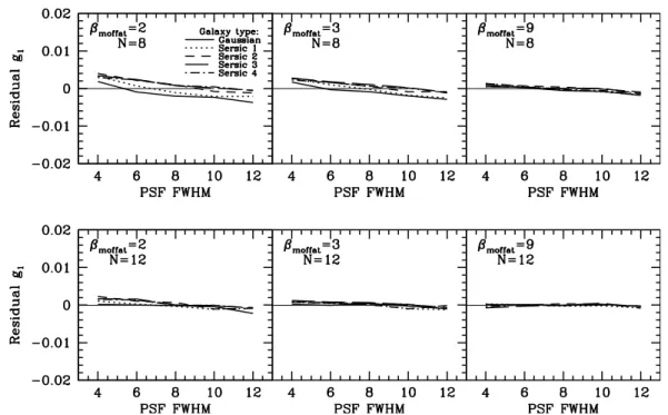
First, to test the “shear calibration” factor, we check how well we can recover the shear of a galaxy that is sheared by
g1 = 0.1 and convolved with a round PSF. Figure 5 shows the result: any calibration error is at the sub-percent level; the worst results are obtained for the most non-Gaussian PSFs (βm =2). The noise in the curves suggests that we are also limited by the accuracy of the Monte-Carlo simulations of the galaxies, and by the numerics of the software implementation of the method.
The second test shows to what extent PSF ellipticity pol-lutes the shear estimate. The input PSFs were given an elipticity
e1 = 0.1 (axis ratio 0.82), and convolved with round galaxies. The recoveredeis shown in Fig. 6. The residual effect is at most half a percent (worst case), which represents a correction of the PSF ellipticity by a factor of better than 20. The best results are obtained for lowish Sersic indices (below 2) and for PSFs with not too extended wings (Moffat index 3 or higher). Perhaps sur-prisingly, the larger the PSF (for the same galaxy size) the better the correction: presumably this is a small sampling effect.
Finally, we introduced a lopsided PSF (by giving 1/4 of the photons an extra offset of half theFWHM) and repeated the anal-ysis. As can be seen from Fig. 7, this combination of dipole and quadrupole PSF distortion can also be handled.
In all cases, taking the expansion toN=12 increases accu-racy, though not spectacularly. We conclude that the algorithm works: shapelets provide a promising technique for measuring galaxy ellipticities, and for correcting ellipticities for smearing by the PSF.
4.4. Noise
A final series of tests was used to check the behaviour of the algorithm on noisy images. We added Poisson noise to simula-tions such as those just described, and compared the result of many realizations. The PSFFWHMranged from 4 to 12 pixels, the galaxies’ effective radii were set to 4 pixels. The same ranges of Sersic (0.5–4) and Moffat (2, 3, and 9) indices were used as above, and the input shear was 0.1. Different levels of noise were added, roughly to span the S/N range between 10 and 100.
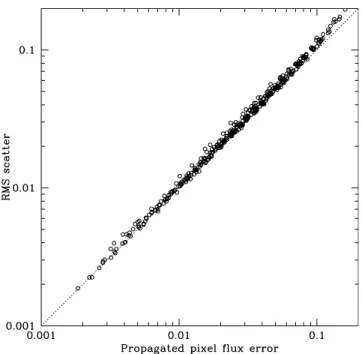
The results are summarized in Figs. 8 and 9, which show that the noise causes a scatter on the ellipticity estimates, but that this does not lead to a bias; and that the propagated error estimates on the ellipticities are a good measure for the rms scatter among the different realizations.
5. The pipeline
832 K. Kuijken: Shears from shapelets
Fig. 5.Fractional error in recovering a 10% shear, using round PSFs. Each panel represents a different Moffat PSF; the rightmost panels are very nearly Gaussian. The simulated galaxies have effective radii of 4 pixels.Top row: 8th-order shapelets;bottom row: 12th-order shapelets.
Fig. 6.Residual shear after correction for an elliptical PSF (the same PSFs as Fig. 5, sheared by 10%).
5.1. Detecting sources
The first step in the reduction process is the detection of sources. For this the SExtractor software (Bertin & Arnouts 1996) is used. A few basic parameters are measured during extraction: position, the flux and its error, theFWHM1, major and minor axis length and position angle, and source quality flags. SExtractor is fast and effective, particularly for the relatively high S/N sources that are used here.
1 FWHMis determined by doubling the FLUX_RADIUS parameter
of SExtractor, and not theFWHM_IMAGE parameter which is prone to failure at low fluxes.
5.2. PSF maps from shapelets
The PSF is determined from the stars in the image itself. We assume that the pixel values are linearly related to intensity.
Fig. 7.Residual shear after correction for a lopsided PSF (the same PSFs as Fig. 5, but a third of their flux is displaced by (2/3)FWHM).
exactly zero. Finding the required offsets involves solving a sim-ple linear equation. Each shapelet is finally normalized to unit integral, by analytically integrating the counts in each shapelet term and dividing by the total.
Once this is completed, we have a shapelet description of (candidate) PSF objects scattered over the image. A map of the PSF variation across the image can now be made by interpolat-ing the shapelets. We have found that a straightforward polyno-mial fit, coefficient by coefficient, works well, though complex PSF variations may require more sophisticated schemes such as weighted nearest neighbour averages (Christen 2006), Padé in-terpolants (Hoekstra 2004), or even physically-motivated model fits (Jarvis & Jain 2004; Jain, et al. 2005). During the fitting of the variation of each coefficient over the image, deviant points can be rejected, leaving a cleaned sample of PSF objects.
The result of this step is a recipe for the shapelet coefficients of the PSF at any point in the image.
5.3. Shapelet encoding
Once the PSF is determined, all other detected sources are ex-pressed as shapelets as well. As for the PSF objects, a shapelet expansion centered on the SExtractor coordinates, is fitted di-rectly to the observed pixel values. The statistical errors on the pixel values are propagated through the least-squares fitting, leading to errors (and if desired, covariances) on the shapelet coefficients. In the case of well-resolved shapelets and uniform noise level across the source, the shapelet normalization is such that the rms error on each coefficient is the same, and the corre-lation between errors on different coefficients small.
Each source is encoded into shapelets with scale radius de-rived as described in Sect. 4.2. All pixel values within a radius of 4βfrom the SExtractor centroid (at least 10 pixels) are used in the fit. For efficiency reasons in the shear estimation step, the al-lowedβvalues are quantized: allowed values areβ =2n/8β
psf, n = 0,1,2, . . .After fitting, the center of expansion for each object is shifted in the image plane by means of the shapelet translation operators until the 01 and 10 coefficients are zero, as before.
This procedure describes the source as seen in the image plane, i.e., after it has been convolved with the PSF and pix-elated. An alternative approach also make sense: to convolve all basis functions with the pixelated PSF, and fit the observed source image as a combination of those. This yields a shapelet description for the intrinsic, pre-seeing, object shapes (Massey & Refregier 2005). As long as the same procedure is followed for the sources and PSF, the end result should be the same: the deconvolved image will be free of pixelation and PSF. We prefer our approach because it leaves the covariance between the fitted shapelet coefficients small.
All sources are encoded to the same shapelet order as the PSF (typically 8 or 12), in order to avoid signal-to-noise depen-dent smoothing effects. For faint sources, the higher-order coef-ficients will therefore be very noisy, but still unbiased.
5.4. Shears from shapelets
With a description of the shape of each source and the corre-sponding PSF, the next task is to determine the intrinsic shape parameters that are needed for a weak lensing analysis.
As explained in Sect. 3.3, we derive the ellipticity as the shear that needs to be applied to a suitable round source in or-der to fit the observed image. The fit is applied completely in shapelet space. We use a scale radius equal toβ2−β2
psf 1/2
for the intrinsic, deconvolved, circular model galaxy, and normalize all sources to unit flux before fitting so that es withβ > βpsfare used. TheCnmlconvolutthecncan be used as radial profile shape
parameters. Only sourcion coefficients need to be evaluated only once per value ofβ.
5.5. Cleaning the catalogue
The resulting catalogue of sources with shape estimators needs to be cleaned in order to remove sources which are affected by neighbours, edge effects, poor fits, etc. We apply various cuts:
834 K. Kuijken: Shears from shapelets
Fig. 8.The result of Monte-Carlo simulations, in which many noise realizations of Sersic profile galaxies were run through the ellipticity-fitting procedure described in this Paper. Shapelet orderN=8 was used throughout. Each plotted dot represents the average ellipticity of 2500 different noise realizations of the same galaxy image. The same data are plotted in both panels, but coded by different model parameters: the Sersic index on the left, and the PSF size on the right. The vertical axis shows the fractional scatter of the measured fluxes,σ(F)/F, of the sources, as determined by integrating their shapelet series. No trend of the mean shear with S/N is seen: noise leads to scatter but no bias.
2. Unresolved and faint objects. Next size and S/N cuts are applied to the catalogue: typically all objects with best-fit Gaussian radius smaller than 1.1 times that of the PSF, and those with flux less than 10 times the flux error (as measured by SExtractor parameters FLUX_AUTO and FLUXERR_AUTO), are removed.
3. Shape cuts. For the next cut, for each source the fraction of powerFnat each ordernin the shapelet expansion is
calcu-lated. An unusually high amount of power at high order, par-ticularly for oddn, indicates a source whose shapelet expan-sion is affected by a neighbour. Thresholds are set for each
Fnbased on the properties of the ensemble population, above
which sources are rejected. Typical values are F3 > 0.05, F4 >0.2,F5 >0.1,F6 >0.2. By constructionF1 =0, but to filter out peculiarly lopsided sources a maximum can be imposed on the distance by which the center of the shapelet expansion had to be moved in order to set the 10 and 01 co-efficients to zero. No cuts are applied toF2since that would be similar to a cut on image ellipticity.
4. Radial profile cuts. As a by-product of the shear estimation, radial profile parametersc0. . .cN−2are generated. These can be used to further excise peculiar objects. If the shapelet
scales are chosen properly and the shear fit worked well, most of the flux of the pre-seeing, pre-shear model source should be contained in theC0 term. Catastrophic failures of the fit, or problems with the setting of the shapelet scale, can be identified as peculiar values ofc0. Requiring|c0−1|<0.5 filters out such cases.
5.6. Average shear
Once individual estimates have been obtained for each source these need to be combined in some way to generate a shear esti-mate.
Conceptually the simplest methods are (i) to average theei
and divide by (1− e2) (Eq. (9)), and (ii) to identify the mode of the ellipticity distribution (provided it is centrally peaked), which identifies the intrinsically round galaxies.
Fig. 9.Comparison between the scatter in ellipticity measurements from sets of 2500 random noise realizations, and the error predicted by prop-agating the pixel noise through the calculations.
procedure, and the former can be estimated as the excess vari-ance ofein the source population. We therefore adopt individ-ual weightsw=(s2
e+σ21+σ22)−1when forming the mean of all measured ellipticities.
The same weighting is then applied to determine the value of (1− e2) in Eq. (9). So the shear estimate is determined as
w=(s2e+σ12+σ22)−1 (18)
e2= w(e 2
1+e22)−w(σ21+σ22)
w −
w e1
w
2
−
w e2
w
2
(19)
gi=
1 1− e2
wei
w · (20)
The value ofs2
e in Eq. (18) can be iteratively adjusted to equal
e2 from Eq. (19), though its precise value is of little conse-quence.
Depending on the form of the intrinsic shape distribution of galaxies, different weightings are optimal: for example, for a very peaked distribution of ellipticities higher weight can be given to nearly round sources, whereas for a top-hat distribution the sources with large ellipticity carry more information – for a discussion see BJ02. A problem with weight factors that depend oneis that the centroid needs to be found first as it is the intrin-sic, pre-shear ellipticity that counts. The weight adopted above is optimal for a Gaussian distribution of intrinsic ellipticities.
In the tests below we will compare the weighting scheme just described, and a simple unweighted median. To the extent that the median identifies the center of the distribution of ellipticities of the source population, i.e., the intrinsically round sources, no (1− e2) correction needs to be applied to the median.
6. Tests on STEP1 data
A rather realistic test of the whole procedure is provided by the “Shear Testing Programme” (STEP, Heymans et al. 2006).
Table 1.Summary of the results of the STEP1 simulations. For each PSF, the slopem1and interceptsciof the best-fit linear relation between
input and recovered shear are shown. Theci have been multiplied by
100 for clarity. As no inputg2 distortion was applied in the STEP1
simulations,m2cannot be measured.
Weighted Average Median
PSF m1 c1 c2 m1 c1 c2
0 0.995 −0.02 0.03 0.982 −0.03 0.01
1 1.005 0.06 0.22 0.981 0.01 0.12
2 0.963 0.19 0.38 0.967 0.02 0.07
3 1.009 0.00 0.03 0.984 −0.02 0.02
4 1.010 −0.01 0.02 0.986 −0.02 0.01
5 1.012 −0.01 0.03 0.988 −0.04 0.02
Phase 1 of STEP has produced a large set of realistic simulated images across which a constant shear (ing1) and PSF smearing has been applied. The PSFs mimic realistic optical aberrations. These images provide an important test, since unlike the tests presented in Sect. 4, the pre-seeing sources do not have a con-stant ellipticity with radius. Furthermore, the STEP images in-clude photon noise, and the sources may overlap. The PSFs are also somewhat smaller (in pixels) than in the tests of Sect. 3.3: scale radii used range from 2.2 to 3.2.
An analysis of the STEP1 data with an earlier version of this software was reported in Heymans et al. (2006). The main im-provement in the implementation since then has been the use of polar shapelets in the shear determinations, which allows trun-cation effects to be curtailed properly, and the use of larger scale radii as discussed in Sect. 4.2.
Results of the use of the present pipeline on the STEP1 data are shown in Fig. 10. For each of threeg1shear values, and six different PSFs, 64 separate simulated images were run through the pipeline, each image yielding shear estimates based on about 2200 galaxies. Table 1 summarizes the results per PSF in terms of a multiplicative correction factorm, and an additive offsetc. It can be seen that in general the method suffers from very lit-tle bias. For the non-elliptical PSFs (0, 3, 4, 5), the recovery is perfect within the noise (m = 1,c = 0), which indicates that the correction for dilution by PSF smearing works. On the other hand, for the comatic (1) and elliptical PSF (2) there is a resid-ual additive term, of nearly 0.003 and 0.005 in shear respectively. This result is consistent with that of the simulations in Sect. 4.3. In addition the elliptical PSF suffers from a multiplicative bias of nearly 4%. The origin of this discrepancy is not clear at the moment.
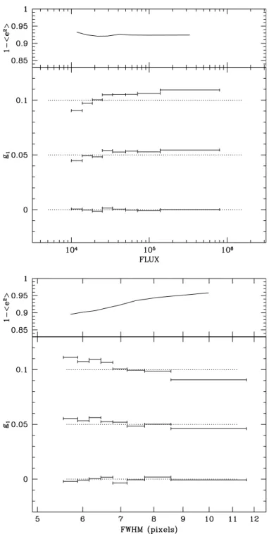
The STEP1 analysis revealed that many methods show a small systematic trend between the error in the derived shear and the magnitudes and sizes of the objects (Heymans et al. 2006). The technique presented in this Paper is no different, as illus-trated in Fig. 12. These trends are still a puzzle, but it is clearly important to trace their origin and further improve the accuracy of the shear measurement. Possible causes include ellipticity-dependent incompleteness in the catalogues, problems esti-mating the intrinsic ellipticity dispersion e2, magnitude- or size-dependent neighbour contamination, or residual systematic issues in the method itself. Further work addressing these issues is on-going.
7. Comparison with other techniques
836 K. Kuijken: Shears from shapelets
Fig. 10.Results from the STEP1 simulations, which are based on mod-eling of the optics of the CFHT. Each plotted point represents the av-erage ellipticity of about 2200 sources in one STEP1 image. Shapelets to orderNmax=8 were used. PSFs 0 to 5 are, respectively, round, with
coma, with astigmatism, with defocus, and with 3rd and 4th-order astig-matism, and results for images with applied shears of 0, 0.05 and 0.1 are shown as three clusters of points in each panel. The correction factor 1− e2is about 0.93 in all cases. Results from cluster to cluster are not
statistically independent, but within each cluster of points they are.
PSF shapes. The correction for the PSF is performed in a sin-gle step, which avoids the need to separate the effect of the PSF into an anisotropic part that shifts the ellipticities, and a round part that causes a dilution of the source ellipticities. The forward-fitting approach of a PSF-convolved model for the in-trinsic galaxy shapes to the observations allows error propaga-tion. The fact that the ellipticities derived are “geometric” in the sense of BJ02 (i.e., they represent the shear to apply to a round object in order to fit the source) means that there is no need to derive a higher-order “shear polarizability”, but instead the re-sponse of an ensemble of sources to shear can be predicted sim-ply from the dispersion in ellipticities.
The use of shapelets in this method is not essential, but does help to speed up the calculations, and gives a natural framework for isolating them = 2 components that carry the ellipticity
Fig. 11.As Fig. 10, but now the median ellipticity is used as shear esti-mator. The STEP1 galaxy ellipticity distribution is very peaked, which makes the median a very efficient estimator of the center of the distri-bution.
information about a galaxy. It also allows the source lists to be filtered efficiently based on objective shape criteria, and gives a robust way of interpolating the PSF shape across an image. In cases where the PSF cannot we well-described by a truncated shapelet expansion (for example, poorly-sampled space-based observations) it is possible to extend the technique, by perform-ing the PSF convolution of Eq. (16) in pixel space instead of in shapelet space (Kuijken 1999).
Fig. 12.The recovered shear for the STEP1 simulations for PSF0 and input shears of 0, 0.05 and 0.1, split up by source brightness (top) and size (bottom). In both cases there is a systematic, so far unexplained trend. The upper panel in each plot shows the ellipticity dispersion cor-rection factor derived for and applied to each bin.
The approach we have taken here differs in several ways from that of Refregier & Bacon (2003) and Massey & Refregier (2005), which is also shapelets-based. We perform the shapelet expansions to a fixed order, and prefer not to introduce signal-to-noise dependent thresholds that may lead to biases in the de-rived shears (S/N dependent truncation and averaging do not commute). Our non-iterative procedure is also much faster. Our shapelet expansions describe the observed, post-seeing images, which means that the coefficients are statistically almost in-dependent (whereas shapelet coefficients of the deconvolved
shapes are necessarily correlated), ensuring that they are vir-tually unaffected by truncation of the series. We explicitly al-low for errors in the centroiding of the sources in our elliptic-ity estimates, and forward-fit the observed images to account for PSF effects rather than deconvolving them using a truncated PSF shapelet expansion. Finally, rather than modeling the response of a (model or empirical) population of images to a shear, we de-rive “geometric” ellipticities (BJ02) for each individual source, and average these only at the end.
Compared to the Bernstein & Jarvis (BJ02) technique, the two main differences are the way ellipticity is measured, and the way PSF effects are handled. BJ02 derive geometric ellipticities by fitting an elliptical Gaussian form to the observed images. This is similar to, but not quite the same as, a low-order shapelet fit as used in this paper. For sources with constant-ellipticity isophotes the BJ02 method is exact, whereas ours is accurate only too(e2) (see Fig. 2). The benefit is a much faster numerical convergence. BJ02 correct the ellipticities for PSF convolution by means of a description of the PSF as a Gauss-Laguerre ex-pansion (equivalent to polar shapelets). Optionally, the images can be convolved with a rounding kernel before the ellipticities and PSF are measured, in order to improve the accuracy of the PSF model. Thus the main difference with the approach here is that BJ02 first derive a post-seeing ellipticity, which is then corrected for the PSF; here we forward-fit the intrinsic ellipticity in one step. BJ02 separate the effects of PSF anisotropy (elliptic-ity bias) and circularly-symmetric smearing (elliptic(elliptic-ity dilution). They correct for the latter by assuming an intrinsic light profile of the source that is a perturbation about a Gaussian, expanded up to the kurtosis. The fact that here we model the full intrin-sic radial profile of the source as higher-order shapelets should provide higher accuracy.
The Kaiser (2000) technique is a more sophisticated kernel convolution technique, in which a convolution kernel is con-structed which turns an image into one for which the effect of pre-seeing shear on all sources is known exactly. This allows one to find the shear that makes the source ellipticity distribution isotropic – this is then the opposite of the amount by which the population was sheared on its way to the telescope. The method is in principle exact, and operates in pixel space. It appears to have received relatively little use thus far (Wilson et al. 2001a,b; Dahle et al. 2002).
8. Conclusions
Shapelets provide a neat framework in which to describe the transformations that an astronomical source image undergoes until it is registered on a detector. Gravitational shear, convo-lution with a PSF, and pixelation can all be modeled within the shapelets formalism. All these elements can be combined into an efficient algorithm for extracting image ellipticities that can be used for accurate gravitational lensing shear measurements.
The implementation of these techniques into a working pipeline is presented in this paper. Tests show that the pipeline is able to recover input gravitational shears with very small cali-bration error (of the order of a percent) and PSF residual (better than a factor of 30 in PSF ellipticity).
838 K. Kuijken: Shears from shapelets
Acknowledgements. Ludo van Waerbeke provided the simulated “STEP” im-ages used in Sect. 6. The Leids Kerkhoven Bosscha Fonds is thanked for travel support.
Appendix A: Circular shapelets
The Cartesian shapeletsSab at ordern = a+b can be written as inhomogeneous polynomials inxandyof combined ordern
times a circular Gaussian. The leading-order term forSab(x, y) is (R03)
2nkxaybe−r2/(2β2) (A.1)
wherekis a constant that is independent of order, andr2 =x2+
y2. The circular shapelet at (even) ordernis the unique linear combination of theSabwitha+b=nthat depends only onr: to
leading order inr Cn(r) ≡ki=0,2...,n
n/2
i/2
Si,n−i(x, y)
=2nkkx2+y2n/2e−r2/(2β2)
, (A.2)
wherekis chosen to normalizeCnto unit integral over thexy
plane. From the fact that rotation of Cartesian shapelets only mixes terms of the same ordern =a+bit follows that the lin-ear combination in Eq. (A.2) is circularly symmetric at all orders ofr.
References
Bernstein, G. M., & Jarvis, M. 2002, AJ, 123, 583 (BJ02) Bertin, E., & Arnouts, S. 1996, A&AS, 117, 393 Christen, F. 2006, Ph.D. Thesis
Dahle, H., Kaiser, N., Irgens, R. J., Lilje, P. B., & Maddox, S. J. 2002, ApJS, 139, 313
Erben, T., Van Waerbeke, L., Bertin, E., Mellier, Y., & Schneider, P. 2001, A&A, 366, 717
Heymans, C., Van Waerbeke, L., Bacon, C., et al. 2006, MNRAS, 368, 1323 Hoekstra, H. 2004, MNRAS, 347, 1337
Hoekstra, H., Franx, M., Kuijken, K., & Squires, G. 1998, ApJ, 504, 636 Hoekstra, H., et al. 2005, preprint[arXiv:astro-ph/0511089] Jain, B., Jarvis, M., & Bernstein, G. 2006, J. Cosmol. Astropart. Phys., 2, 1 Jarvis, M., & Jain, B. 2004, preprint[arXiv:astro-ph/0412234] Jarvis, M., Bernstein, G. M., Fischer, P., et al. 2003, AJ, 125, 1014 Kaiser, N. 2000, ApJ, 537, 555
Kaiser, N., Squires, G., & Broadhurst, T. 1995, ApJ, 449, 460 (KSB) Kuijken, K. 1999, A&A, 352, 355
Luppino, G. A., & Kaiser, N. 1997, ApJ, 475, 20
Mandelbaum, R., Hirata, C.M., Seljak, U., et al. 2005, MNRAS, 361, 1287 Massey, R., & Refregier, A. 2005, MNRAS, 363, 197
Press, W.H., Flannery, B.P., Teukolsky, S.A., & Vetterling, W.T. 1986, Numerical Recipes: The Art of Scientific Computing (Cambridge University Press) Refregier, A. 2003, MNRAS, 338, 35 (R03)
Refregier, A., & Bacon, D. 2003, MNRAS, 338, 48 Rhodes, J., Refregier, A., & Groth, E. J. 2000, ApJ, 536, 79 Schneider, P., & Seitz, C. 1995, A&A, 294, 411
Sersic, J. L., Atlas de galaxias Australes