ABSTRACT
Women’s occupation choice has been incompletely modeled in the past, but this paper brings together several methods to seek a more complex understanding of the decision process. I employ panel data spanning three decades (1979 to 2012) and six thousand women in the United States to investigate the impact of childbirth on the mother’s decision between occupations. I use a multinomial logit model estimated through Stata’s generalized structural equation modeling software and incorporate expected potential incomes through multiple imputation. Instrument variables for childbirth expectations are employed to address endogeneity. Issues of endogeneity ultimately turn out to be troublesome to correct for, but estimates from several models indicate that women with children are less likely to work as managers and more likely to choose
ACKNOWLEDGEMENTS
SECTION I:INTRODUCTION
Starting in 1965, Gary Becker took the microeconomic analysis of the household to new levels by focusing on the production activities of household members. His efforts opened a new field of study within microeconomics that has continued to bear fruit over many decades (Becker 1991). Since Becker expanded microeconomic analysis to the non-market domains of individual human behavior and interaction, we can now model household decisions in a marginal-cost and marginal-benefit framework in which the agent seeks to optimize his or her utility subject to budget constraints. Analysis of behavior and decisions at the household-level has flourished, providing economic models of marriage, divorce, and fertility. Following Becker’s pioneering work and the expansion of that work by countless others, I seek to model a woman’s decision between occupations in a utility maximizing framework in which she chooses a particular occupation that provides her with more utility than other available options.
Previous studies have considered the decision to work as a binary variable in which a mother allocates her time between work and non-work (i.e. household production) areas. Other papers have modeled general occupation choices, but with little focus on how children could potentially affect this decision. However, factors such as previous investments in future careers and the presence of children have a non-trivial effect on not only whether, but where, women choose to work.
potential utility gained directly from holding such a position, and other occupations which would allow for more time flexibility.
Women’s time allocation among work and household production has remained the subject of much debate as women continue to lag behind men in earnings and labor force participation (F. D. Blau and Kahn 2007). Even though gender inequity in the United States has greatly improved over the last several decades, among married couples who have children, women much more often than men must choose between work and home production activities (i.e. childrearing) (Crittenden 2000). The continuation of gender-based division of childcare and housework makes it difficult for women to successfully combine pursuing a career with raising a child (Shreffler and Johnson 2013). High daycare costs present an additional barrier when the expected income from working does not cover the cost of ensuring high quality childcare in her absence. Blau and Robins (1991), Barrow (1999), Connelly (1992), Kimmel (1998), Powell (1997), and Ribar (1992) all found that childcare costs negatively affect women’s likelihood of being in the workforce. In this way, the presence of children in a family can significantly change the way a woman makes her decision about work.
I first hypothesize that there is a difference in occupation choice between women with children and those without. I expect that this can be explained by changing preferences for job characteristics such as flexibility, attractive family leave policies, and low atrophy rates. Further, I hypothesize that women with children are less likely to choose jobs classified as professional and managerial. I expect this is the case because occupations such as clerical and service work require lower investments of time which makes them more attractive to risk-averse mothers, despite the higher income potential offered by professional and managerial jobs.
The hypothesis that professional and managerial jobs are particularly less prevalent among women with children stems from prior research as well as theory in utility maximization. Ma (2010) finds that professional females experienced a substantial reduction in utility compared to their nonprofessional counterparts due to the presence of young children, and her findings are mirrored by Johnes (2009). In a utility maximization framework (further explored in section II), attributes such as low flexibility have a more significantly negative impact on her utility given the presence of children, leading to a choice of occupation which offers more desirable job attributes.
The research presented here confirms that children and occupational choice are intimately connected, using panel data from the National Longitudinal Survey of Youth (1979). It
incorporates not only market variables such as wages and family income, but also the systematic variation in preferences among women that leads to differing choices.
decision to work varies by occupation choice, I am interested in how women decide between occupations given they have chosen to have children. My primary addition to the current available work on this subject will be to analyze this decision explicitly. Unlike many previous studies, I use panel data to analyze the occupation choice over time and incorporate more
rigorous econometric procedures in the hopes of successfully modeling the interrelated nature of the decisions at play. Additionally, I depart from prior research by carefully addressing threats to internal validity which would be introduced by assuming presence of children and work status to be exogenously determined. Instead, I account for selection bias by including the decision to work in the occupation choice and reverse causality by implementing instrument variables. Finally, I update the results of previous studies performed in the 1980s and 1990s to provide analysis of women’s occupation choice through 2012.
SECTION II:THEORETICAL MODEL
A. Stage 1: Before Childbirth and Marriage
As a baseline model for women’s occupation choice, consider a single young woman, age eighteen, who has no children and is in the process of deciding whether to go to work or to continue her education. Her decision tree consists of two base branches: start work immediately or acquire further training in the form of education. Her choice between these two branches depends on her individual preferences and on the resources she has available. If she prefers to begin work immediately, she will by assumption choose among the occupations that offer the greatest utility. The utility criteria for this decision will include at minimum current pay levels, future pay levels, compatibility with her nonmarket activities, and nonpecuniary characteristics of the occupations available to her. These nonmarket activities refer to home production activities, which in the future may include marriage and children. On the other hand, if she decides to continue her education, she puts off for some time a choice as to careers. The continuation of education does, however, offer her a wider range of future occupations from which to choose. During the training, she may also make decisions about which occupations to seek after finishing her education. That is, in seeking further training, she may specialize in a certain area which narrows her future choice. Her eventual career choice will also depend on the same criteria that guide the occupational choice of a woman who does not continue her
education.
obligations. Men, on the other hand, have historically only had to focus on the characteristics of the occupations themselves without considering how the occupation might affect their
hypothetical future marriage and family. Women’s labor supply decisions and occupational choice decisions are therefore considerably more complicated than those of their male counterparts.
For example, the young woman making a decision to work today might not care about the attractions of the myriad available jobs if she expects to marry and quit her job in the not-distant future. She might search for a job that is easy to exit and has opportunities to reenter later on should she desire. Decades ago, women chose these sorts of professions with the expectation that they would soon leave their job upon marriage or childbirth. They sought occupations which did not require extensive time dedication, knowing that they would likely not be present to reap the rewards of such devotion to the job. Teaching, nursing, and secretarial positions (and, although less high-status, retail and food service jobs) required fairly minimal training and education (in comparison which that required to become a doctor, engineer, business-person, etc.) and did not demand long hours in the office.
Over time, it is clear that expectations of women’s current and future nonmarket
obligations have changed. The weakening emphasis placed upon on women to remain at home to rear their children changes the importance they place upon certain job characteristics. As
A woman choosing to continue her education might do so in order to increase the
attractiveness and variety of future jobs, to make herself a more desirable option on the marriage market, or a combination of the two. Continuing her training, therefore, does not necessarily suggest that she is more dedicated to having a long career. Her decision to continue her schooling is based in several factors, only one of which is the hope of increasing her job opportunities.
Conventional labor supply models have traditionally focused on a woman’s preferences for “leisure” time and consumption of market goods obtainable with wage income (Borjas 2010). These models do not typically account for systematic differences in the tastes among women, particularly as they relate to parenthood. However, one can make the case, as this paper does, for non-random variation in preferences for work and home time allocation across demographic characteristics like race/ethnicity, age, education, socioeconomic status, geographic location, degree of urbanization, and marital status. These variations in preferences are particularly important for women as compared to men for reasons previously discussed. A woman may be more willing than a man to trade salary for job flexibility so that she can take on home
responsibilities. She may also be willing to accept lower wages for occupations that have attractive nonpecuniary characteristics.
In the case of women who choose to go to work immediately, it is likely that they see their occupation in instrumental terms; that is, they see their work as a means to an end: income and/or a set of preferences relating to marriage and family. Women who choose to obtain higher education are both expanding their options and complicating their choices. Because these women will be educated in a way that brings the nonpecuniary characteristics of a job into greater
compatibility with nonmarket activities such as marriage and child-rearing. Such career benefits might include the pride of having reached a high-level position in the company or independence derived from being fully self-supporting.
We model this decision to work as a utility maximizing decision. Following Becker (1991), the agent divides her resources between work and home production. She operates as a utility maximizer who derives her utility from home time and the consumption of goods using income obtained from the market. She also gains utility from working that is independent from the income achieved thereby. There is an evident economic tradeoff between working in order to consume goods (and reap the non-pecuniary benefits) and staying home in order to produce home goods, which also provide utility and require market income as an input (Borjas 2010). The woman’s utility function is defined as follows:
(1) = ( , ; )
The same factors that determine her decision between continued education, career, and home production also bear weight in her occupation choice. For both women leaving high school and those leaving college/higher education who have decided to work, choosing between
occupations changes the amount of utility gained from working. Following DeLeire and Levy (2004), the utility gained from this decision depends on her expected wages, the attributes of the job, and her individual characteristics.
Demographic characteristics, particularly the level of education, are integral to the occupation choice because they may limit the available job options as well as place a greater weight on certain job attributes. For example, a woman with a lower educational background might not have the same opportunities for meaningful employment, and thus may be severely limited by which occupations she can chose. A woman who has dedicated many years to her education is likely to place more importance on receiving a high salary to offset school debts and the opportunity cost of having not worked all those years she was in school. She may also seek out job attributes which allow her to make use of the skills she honed at university. Another clear example of variation in occupation choice due to demographic characteristics is the effect of the woman’s location.
Although she is unconstrained by marriage and children in the current time period, she may take into account future expectations when making her current occupational choice. Her opinions about the distribution of home and work time between herself and her future spouse could limit her from choosing certain careers. A woman who expects that her husband will work while she stays at home might be considerably more likely to choose a career which does not require a large investment of time up front in exchange for later benefits and upward mobility. A woman who hopes to marry and have children in the future may well expect that her choice of occupation should allow her this alternative. This might entail easy entry and exit from her job and potential to work part time in order to balance family and work. In this way, her future expectations about the path of her life could significantly impact her present job choice.
The importance of certain job attributes also varies among individuals. Previous literature modeling occupational choice has identified several different qualities which might be of
are randomly determined. None of these papers address occupational choice as it is affected by the presence of children, but their inclusion of job attributes provides a basis for this paper. Occupation choices are expected to vary across women with or without children depending on their changing preferences and needs for certain job attributes, such as flexibility, maternity leave, and low rate of skill depreciation.
Given that she has decided to work, her utility function now additionally depends on the type of occupation the young woman chooses. She seeks to maximize her potential utility, so following Blott (2012), she chooses an occupation j for which utility is greater than for any other occupation k.
(2) > ∀ ≠
(3) = ( , , ; , )
This occupational utility depends on expected wage rate (W), job attributes (A), and individual characteristics (X) (DeLeire and Levy 2004). It also depends on her individual preferences for work (PW) and for children (PC).
If life were simpler, a labor supply function could be derived from this utility function, from which we could ascertain information about the relative importance of income and substitution effects. However, because her utility depends on varying characteristics and preference that cannot be assumed to be randomly distributed or equivalent across all women, the functional model becomes far too complex to derive a straightforward supply function. Nonetheless, defining the young woman’s occupational utility provides a theoretical basis for analysis, one which can be modified to describe the young woman at later stages in her life. It translates into the diagram in Figure 1which models the occupation choice based on various determinants which positively or negatively influence the utility gained from any occupation j. We now revisit this woman after she has married and had at least one child.
B. Stage 2: After Childbirth
With some adjustments, we use the same woman’s earlier occupational choice model to describe the decision she makes regarding her occupation after she has her first child. The previously determined variables provide a baseline for a woman’s occupational choice and labor supply decisions. The occupation she chooses still depends on her expected wage rate,
demographic characteristics, and current preferences for home/work division. She seeks to optimize the utility she can gain from working by choosing the occupation that best fits her characteristics.
choosing not to have children. Commitment to an occupation that requires many years of school and training (such as physicians), for example, would decrease the likelihood that a woman give birth in her early 20s. Past literature does not uniformly approach this endogeneity; many previous studies using cross-sectional data ignore the issue altogetherand others mention it without attempting any model corrections (Ribar 1992; Shreffler and Johnson 2013; Johnes 2009).
Although previous research disagrees on the endogeneity of fertility, all papers make the same assumption about the labor supply of the husband. Ribar (1992), Ma (2010), and Barrow (1999) explicitly incorporate husband’s income and work status into their models and assume that these variables are exogenously determined. Ma additionally operates under the condition that the husbands all work full time, as do the women themselves. Since we are revisiting these women after they have married and had at least one child, we will treat their spouse’s income as predetermined in the structural models that follow.
The presence of children implies that the woman is either married or a single mother. We limit this discussion to women who are either married or cohabiting (i.e. not single) in order to develop a model, acknowledging that single mothers too face a job choice, albeit one that is severely limited by the available childcare and income potential. Other preferences may exist, but not carry a heavy weight in their decision-making process in comparison to the strong importance income carries. In the case of a married mother, her total household income is now equal to the sum of her own expected wage rate and the predetermined wage rate of her spouse.
dedicated her life to reaching a certain career goal would find it difficult to switch occupations in favor of one that provides flexibility and shorter hours so that she can spend time with her child. On the other hand, a woman who prefers to remain at home with her children would be much more anxious to choose an occupation which affords her the flexibility she needs.
In addition to the limitations imposed by her own preferences, the decision to switch occupations is also complicated by external considerations. The labor market is far from perfectly flexible; its rigidity restricts the pool of job options available. A woman may seek a new career but struggle to find available employment. A profession’s requirement of full-time work also limits women from choosing their theoretically optimal work status. There are many jobs that a woman could continue on a part-time or more flexible basis if the labor market were more flexible. Despite the recent popularity growth of some options offering flexible hours have (such as Uber), in most occupations the expectation of 40+ hour work weeks limits women who might ideally seek to split their time between work and home (“The Uber Story” 2017). Thus labor market rigidity introduces an external constraint on the decision to be made.
Preferences are not always time constant. In addition to prior opinions, the mother’s current tastes for work and home production are of equal importance to include. Many working professional women have told a similar story about being fully dedicated to and satisfied with their career, only to find these feelings crumbling as soon as their first child was born. Despite previously insisting that she would never be “one of those women” who quits her job in favor of staying home with her children, she finds herself unable to hand over her newborn child to a nanny or daycare when the time comes to return to her job (Slaughter 2012).
After giving birth, a mother’s utility additionally depends on the quality of the child she and her partner produce. Becker (1991) labels this the “production of z-goods” – the goods produced by the household which require inputs of time and market wages. He sees childbearing as a home production activity which uses parental time and money inputs. The utility gained from this activity is derived in part from the quality of care the child receives, which depends on parental time inputs as well as the quality of outside care services. Most outside childcare options are costly – nannies, daycares, and schools – but a necessary expense if both parents are to work. The parents’ market and home production time inputs are substitutable to a point, but not
perfectly elastic. The elasticity of substitution between market and home production depends on the parents’ relative incomes and tastes for work and childcare.
The woman’s utility after giving birth to her first child now depends on the consumption of goods and time spent in household production of z-goods (Becker 1991). She receives utility from the quality of care her child is given, which is partially dependent on the time she spends with him or her.
Leibowitz and Klerman (1995) incorporate children (N) and the quality of childcare (Q) into the mother’s utility function. The utility she derives from work is a function of consumption and home production, as well as the quality of care her child receives and the presence of
children. Individual characteristics (X) and tastes for work (T) are also included as before the woman had a child.
(4) = ( , , ; , )
The mother’s occupational utility function can be expressed by a similar formula to that before she had her first child, but with the added inputs of past, current, and future preferences, her prior occupation (O), and childcare costs (H), which provide a quantification of the quality of her children.
(5) = ( , , , ; , , )
Figure 2. Diagram modeling the theoretical inputs into a woman’s occupational utility after children, assuming she is married or cohabiting. This diagram corresponds to the utility function given by equation (5).
Although professional and managerial occupations tend to provide higher wages, which may be more important to a woman who must consider the costs of childcare and saving for her child’s future, my hypothesis that women with children will be more likely to choose other occupations is also grounded in previous research. Polachek (1981) found that those with the greatest home-time are least likely to enter managerial and professional occupations. He attributed this to the high atrophy rates of professional and managerial occupations, which lead to large losses in earnings potential if skills are not continuously used.
SECTION III:DATA
This paper makes use of panel data taken from the 1979 cohort of the National Longitudinal Survey of Youth (NLSY79). The study began in 1979 when respondents were between 14 and 22 years of age and continued until 2012, at which point respondents ranged from 47 to 56 years old. This sample of American youth was born in the mid-1950s to mid-1960s and were coming of age in the 1980s. 12,686 individuals were initially interviewed, but
9,964 remained after two sub-samples were dropped in 1990 (“The NLSY79 Sample: An Introduction” 2016).
The survey includes questions about labor market behaviors, income, education, fertility, marriage, health, geography, family background, crime, and attitudes. The employment and fertility information was collected in an “event history” format, noting the start and end dates of important events such as jobs and births (“The NLSY79 Sample: An Introduction” 2016). This format allows for precise calculation of experience at current job and differentiation of women who have given birth. In certain years, additional questions about job characteristics were asked, which will provide context in this paper for the difference in occupations.
Although one of the best available options for this analysis, the NLSY79 is not without its weaknesses. Biannual interviews were implemented after 1994; previously interviews
First, the categories are defined following the Bureau of Labor Statistics coding, which changes four times over the course of the survey. When recoding this variable, it is possible that mistakes were made, introducing error into the econometric models. Second, the categories do not account for a type of occupation which has gained popularity in the past several years: the
“momtrepreneur” (Henault 2016). These women are primarily home-based to care for their children, but have taken on a side venture for additional income and/or to fulfill a passion. Because they can do this work at night or while their children are at school, they are able to combine childcare and work without facing a severe economic tradeoff.
Primarily, data on marriage, education, fertility, and labor market behavior was extracted from the overall NLSY to form the basis of the paper’s dataset. Additional variables related to attitudes toward work and family life were also taken from the NLSY to serve as proxies for latent individual preferences. The dataset spans the entire survey length, from 1979 to 2012. Table 1 in the appendix provides a description of all variables in the dataset. A summary of key explanatory and dependent variables is included in Table 2 below.
Variable Obs Mean Std. Dev. Min Max
Occupation 119,243 3.316 1.985 0.000 6.000
Presence of first child 153,196 0.023 0.151 0.000 1.000
Income 115,771 12680.750 19526.660 0.000 343830.000
Income of spouse 153,196 10264.390 25828.930 0.000 309409.000
Race 153,196 2.434 0.751 1.000 3.000
Region 153,196 3.160 1.323 1.000 5.000
Education 119,716 12.670 2.390 0.000 20.000
Urban 113,549 0.783 0.412 0.000 1.000
Tenure 153,098 2.566 4.434 0.000 37.865
Status (cohabiting or married) 64,031 0.125 0.330 0.000 1.000
Married 119,370 0.942 0.993 0.000 5.000
Age 153,196 32.059 9.830 14.000 55.000
Table 2. Summary statistics of key variables reported for entire dataset.
consistent increasing trend; in 1970 the mean age was 24.6 and by 2000 this number had risen to 27.2 (Mathews and Hamilton 2002). In comparison, the average age of women giving birth in this sample increased each year (see Figure 3in appendix), but this is entirely explained by the increasing ages of the women being sampled. A variable measuring the presence of children was created for each respondent i using the birth year of each respondent’s first child, if one existed. This binary variable equals 1 for respondent i in year t if she had her first child in that year. As expected, the number of births significantly decreases with age; by 1993 the average age of mothers at the birth of their first child was 30.8 and the number of women in the sample giving birth to their first child was less than 100 (see Figure 4). In comparison, at the peak age of first birth, around age 22, there were close to 400 women in the sample who gave birth to their first child.
Figure 4. The number of women giving birth to their first child by year, 1979 to 2012; and by age, 14 to 43. There is a noticeable decreasing trend, with the majority of first births occurring in the early 1980s, and among women in
their early 20s.
By far the most common relationship among women giving birth to their first child is a marriage, with only a few women giving birth while in a relationship with a partner that was not a marriage (this is succinctly referred to as cohabiting). More common than mothers with
0 1 0 0 2 00 3 00 4 00
1980 1990 2000 2010
[1] Gave birth to first child
First Child Birth by Year
F re q ue nc y
Survey year, 1979-2012 Graphs by Binary, =1 if gave birth to first child
0 1 0 0 2 00 3 00 4 00
10 20 30 40
[1] Gave birth to first child
First Child Birth by Age
partners is the single mother – as Figure 5(appendix) depicts, about one third of new mothers reported that they had no partner or spouse.
The other main variable of interest is the occupation code, which was measured yearly and defined based on several different census occupation codes. The 3-digit 1970 census codes were used until 2000, after which point the 2000 census codes were implemented. 4-digit codes were used in 2002, then 3-digit codes were used for the remaining years. Table 3 (appendix) provides the broad categories to which these codes correspond.
The categories provided by the census were in some areas too broad, in others much too specific, to be effective in this analysis. Prior studies have all defined occupation categories in different ways. Ma (2010) divides occupational choice into three categories: managerial and professional specialty occupation, home production, or other nonprofessional occupations. Johnes (2009) defines six types of occupations: full-time managerial, full-time non-managerial, part-time managerial, part-time non-managerial, schooling, and home. In coding new categories, I focused on those which might be particularly interesting when analyzing a mother’s job choice. The main categories of interest to this paper’s hypothesis are “Managers and Supervisors” and “Professional and Technical.” Although “Teacher” and “Health Technician” generally fall under the category of “Professional,” these categories were specified separately because they are historically occupations which populated by women (Hoffman 2003). The “Clerical and Service” category was refined to include only low-level service positions; an occupation such as
Figure6. Frequency of occupation categories in 10 year increments, from 1980 to 2010.
Table 4provides the new categories as defined for this paper. As depicted in Figure 6, the Clerical/Service category is by far the most common occupation among respondents, which is at least partly due to the large size of the category – there are many jobs under the general
classification of clerical and service work. Several time trends are apparent: the amount of home-producers drops substantially, and there are more teachers, professionals, and managers – until after 2000, at which point the number of women in professional occupations drops again. Given that the respondents were as young as 15 in 1980, it is intuitive that the number of women without a job would drastically decline between 1980 and 1990.
Redefined Occupation Codes 0 Managers and Supervisors 1 Professional and Technical 2 Clerical and Service 3 Teacher
4 Health Technician 5 Other
6 Home-Producer
Table4. Occupations as re-defined based on Census Bureau codes. The majority of categories were fused into one category, “Other.” “Home-Producer” refers to women not working outside the home.
Managers Professional Clerical/Service Teachers Health Technicians Other Non-Worker Managers Professional Clerical/Service Teachers Health Technicians Other Non-Worker
0 .2 .4 .6 0 .2 .4 .6
1980 1990 2000 2010 R e sp on de nt 's o cc up a tio n, b y ca te go rie s Density
Graphs by Survey year, 1979-2012
The occupation categories vary across demographics, suggesting the importance of their inclusion in the model. For example, average years of education among respondents who did not work is 12 (i.e. completion of high school), whereas the average among professionals is 15 (several years of college), and teachers have even more education on average (see appendix for Figure 7). Likewise, the plot of occupation categories over race in Figure 8 in the appendix shows that more non-Hispanic, non-Black respondents were in professional and managerial roles than either Hispanic or Black respondents, who were more likely to be unemployed.
Respondent's desired occupation at age 35
Respondent's actual occupation at age 35 Managers and
Supervisors Professional and Technical Clerical and Service Teacher Health Technician Other Home-Producer
Managers and Supervisors 12.15% 8.41% 38.63% 4.67% 3.12% 13.40% 19.63%
Professional and Technical 12.57% 11.27% 39.81% 5.27% 3.11% 11.85% 16.11%
Clerical and Service 8.16% 6.57% 44.64% 4.53% 3.78% 13.44% 18.88%
Teacher 11.29% 6.30% 40.94% 12.86% 3.15% 9.97% 15.49%
Health Technician 7.11% 6.28% 44.98% 3.97% 7.95% 12.97% 16.74%
Other 10.56% 5.87% 36.07% 2.05% 4.40% 20.23% 20.82%
Home-Producer 9.04% 7.81% 42.29% 3.52% 3.47% 14.81% 19.05%
Table 5. The percentage of respondents who were in a certain occupation category at age 35, given the occupation category they desired to be in at age 35.
Figure 9. Distribution of responses to questions about women’s role at home and at work. The six questions were asked in 1979, 1982, 1987, and 2004.
What is perhaps initially most surprising is that respondents begin to disagree more than agree with the question “does a working wife feel more useful?” to the point where in 2004 more women disagreed than agreed. This may seem counterintuitive given that the trend of female empowerment has only grown since 1980, but consider that this figure charts the responses of the same women as they grow older. Perhaps they felt useful and fulfilled working initially, but have grown disenchanted with their jobs by 2004.
Finally, Figures 10and 11 (appendix) give summaries of the occupation categories by certain job attributes. In every category, the majority of respondents had very few females coworkers, but this was particularly true for professionals and managers, and less so for teachers and health technicians. More women in these professional/managerial jobs had male supervisors,
0 .5 1 0 .5 1
Disagree Agree Disagree Agree
1979 1982 1987 2004 D en si ty Respondent's opinion
Graphs by Survey year, 1979-2012
Women's place is in the home?
0 .5 1 0 .5 1
Disagree Agree Disagree Agree
1979 1982 1987 2004 D en si ty Respondent's opinion
Graphs by Survey year, 1979-2012
Wife with family has no time for other employment?
0 .2 .4 .6 0 .2 .4 .6
Disagree Agree Disagree Agree
1979 1982 1987 2004 D en si ty Respondent's opinion
Graphs by Survey year, 1979-2012
Working wife feels more useful?
0 .2 .4 .6 .8 0 .2 .4 .6 .8
Disagree Agree Disagree Agree
1979 1982 1987 2004 D en si ty Respondent's opinion
Graphs by Survey year, 1979-2012
Traditional husband/wife roles are best?
0 .2 .4 .6 .8 0 .2 .4 .6 .8
Disagree Agree Disagree Agree
1979 1982 1987 2004 D en si ty Respondent's opinion
Graphs by Survey year, 1979-2012
Women happier if they stay at home?
0 .2 .4 .6 .8 0 .2 .4 .6 .8
Disagree Agree Disagree Agree
1979 1982 1987 2004 D en si ty Respondent's opinion
Graphs by Survey year, 1979-2012
whereas more health technicians had female supervisors and clerical/service employees were almost equally split among male and female bosses.
SECTION IV:EMPIRICAL MODEL
The theoretical model implies that the decision to choose a particular occupation depends on individual demographic characteristics, characteristics of the job, contributions from the spouse (if existing), expected wage, and work-family preferences. Figure12 (on the following page)shows the relationship between these theoretical variables and those used in the empirical model which are observed in the dataset.
Specifically, these individual characteristics are age, race/ethnicity, geographic location, urbanization (urban or rural), and level of education. Questions about traditional ideals and expectations for time spent at work and home were used to create an index of work-household preferences labelled “Traditionality.”1 Following Ma (2010), Barrow (1999), and particularly
Ribar (1992), I treat the spouse’s contribution as predetermined and therefore exogenous. I can justify this because I am modeling these women at a point in their life cycle. In effect, the spouse’s wage and the respondent’s expected wage together provide a measure of the total household income. Like Ribar, I take as given that the spouse will work full-time and contribute a certain wage.
A. Stage 1
Stage 1 is a cross-sectional model of the single young woman with no children at the survey’s start in 1979. Estimation of this model should provide baseline information about the importance of different variables in the woman’s occupation choice before children have been introduced.
(6) , = + , + , , + ,
The occupation choice Ii of individual i in 1979 is given by equation (6). It depends on demographic characteristics, education level, expected income, and the created index measure of Traditionality. Specifically, the vector , refers to race and the vector , , encompasses
region, education, urban, age, wage, and Traditionality. The occupation choice is defined by the following categories:
(7) , =
0
1 ℎ
2
3 ℎ
4 ℎ ℎ ℎ
5 ℎ
6 ℎ −
There are two serious forms of endogeneity in this model which threaten the internal validity. The first results from self-selection. Because the agent chooses her occupation, it is assumed that the unobserved values where no occupation is chosen are distributed
To account for bias from self-selection, previous studies such as Ma’s exploration of women’s labor supply decision employ Heckman’s two-step model to first model the factors determining the observation of the labor supply choice then estimate the choice conditional on the individual working and vectors of explanatory variables (Ma 2010). However, estimation using the Heckman method necessitates the existence of a variable which could conceivably influence the woman’s decision to work but would not impact her choice of occupation.
Past literature offers up little guidance here; among others, Polachek (1981) implements an instrument for good health, but bad health could certainly skew a woman away from certain occupations and toward others, so its value as an instrument is quite low. Furthermore, the model must be estimated using multinomial logit because the dependent variable is categorical, and there is currently no way to combine Heckman with multinomial logit in Stata.
Instead, the occupation variable was recoded to include a sixth category,
“home-producers,” who do not work. Rather than first estimating the decision to work and secondly the decision between occupations, we estimate the decision jointly, treating unemployment as another occupation category. This model can be estimated using multinomial logit which presents the probability that occupation j is chosen given that woman i is single and the year is 1979. In order to use this model, we assume that the error terms , each have their own
independent standard logistic distribution.
expectation of a certain income determines the chosen occupation. In order to address these issues, I computed a variable measuring the expected income to be received from the given occupation, according to the respondent’s demographic characteristics. Income was imputed using Stata’s multiple imputation with m=20 (convention is to set m to the percentage of missing cases) and the 20 imputations were averaged to develop one value for each missing income. Use of multiple imputation requires us to assume that each variable has its own separate conditional distribution and that the missing values are all missing at random.
The imputation was conducted using the same vector of demographic characteristics that determines occupation choice, plus an instrument proxy for the level of inflation at the time, which is assumed to affect the respondent’s wage rate but be independent of her occupation choice. Leibowitz and Klerman (1995) instead use the regional variation in labor markets as an instrument, which might have been a more robust choice if such a variable were available in the NLSY79.
In the NLSY, what I refer to as “income” is measured by multiplying the respondent’s hourly wage with the number of hours worked. Thus the respondent’s income depends only on the wages she earns and hours she works. Including spouse’s income in the stage 2 and 3 regressions provides a proxy for additional household income. Other forms of income, such as investments and inheritance, were not measured by the NLSY.
B. Stage 2
married or have a partner. Stage 2 is also cross-sectional, but rather than being defined by one year, it is defined relative to the year in which the child is born.
Prior research differs in defining the timing of the decision relative to the birth of
children. Leibowitz and Klerman (1995) analyzed the determinants of work status two years after the first birth. In contrast, Barrow (1999) looked at the decision to return to work quickly, before the first year after giving birth. He focused only on the subset of women who were previously working before they gave birth, a common simplification made by research on women’s labor supply; Paull (2006), Polachek (1981), Johnes (2009), DeLeire and Levy (2004), and Blott (2012) all based their analysis on women who were already working prior to giving birth and are returning to work. This allowed them to avoid the struggle of selection bias due to lack of data on nonworking wages. Their results, for the most part, agree. Low childcare costs, high potential wages, and low family income increase a woman’s likelihood of returning to work. In this paper, however, women who did not work are also included in the analysis. Two models were
estimated: first, in the year of the first childbirth; second, two years following the first childbirth, to determine whether there may be a lag in woman returning to work after their pregnancy.
The basic model remains the same, and the same issues with endogeneity still apply and are addressed similarly. The major differences between stages 1 and 2 are the addition of several variables which might come into play after the introduction of a child to the household. As the theoretical model implies, the choice of occupations seeks to maximize utility determined by demographic characteristics (including the type of relationship), characteristics of the job, expected household income (now incorporating contributions from the spouse/partner), preferences for work and home division, and the prior occupation before giving birth.
of children would be useless in this model because every woman in this cross-section has given birth. Instead, comparison between the stage 2 and stage 1 models is expected to highlight variables for which the addition of having a child impacts their effect on occupation choice.
Consider a woman i at time t+n, where t=1979 and n {0, 1, 2, ..., 33}. Some n years after 1979, she has her first child. Because women with newborn children often take some time to return to the labor force, models estimating occupation choice at time t+n, t+n+1, t+n+2 (that is, with no lag, a one year lag, and a two year lag in childbirth) will be compared. Denote these lags using t+n+m where m {0, 1, 2}. The occupation choice in equation (8) is estimated with multinomial logit as before, which presents the probability that occupation j is chosen given that woman i had a child and is not single. We assume that the error terms , each have their
own independent standard logistic distribution. The same occupation categories are used, provided previously in equation (7).
(8) , = + , + , , + , , + , , + ,
The determinants of occupation choice now include an indicator (status) for the respondent’s relationship type, either married or cohabiting, the predetermined income of her partner, and her occupation prior to having her child. Specifically, the vector , includes race;
the vector , , includes Traditionality; the vector includes , , prior occupation; and the
vector , , includes region, education, urban, age, wage rate, status, and spouse’s wage
C. Stage 3
For the third and final model, I make no restrictions on the year or presence of children. The entire panel is used to estimate the effect of children on occupation choice, with one caveat. I do keep the restriction that the individual is either married or cohabiting. The model of single mothers’ occupation choice differs from that of a mother in a serious relationship in several ways which make it difficult to estimate all marital statuses in one regression. Single mothers cannot rely on their spouse’s wage to supplement the household income, and their single status might interact with many other variables, such as income level, race, and education. Including so many interaction terms would create a very nebulous model. Therefore, this stage is restricted to women in relationships. Several new issues must be addressed when incorporating the panel data.
As this dataset spans from 1979 to 2012, it is likely that changes over time could impact the dependent variable. Figure 6(provided in the Data section) seems to confirm this suspicion. Over the years, the popularity of certain occupations and the availability of certain jobs has not remained constant. Year fixed effects will be implemented in the form of dummy variables for each year to control for this time variation in the error term. The fixed effects method is chosen rather than random effects because it is unlikely that the explanatory variables , are uncorrelated with the error term , .
From the other direction, having children is expected to impact whether a woman decides to work and what occupation she chooses. To address reverse causality, we predict the presence of children separately modeling it on demographic determinants and including instrument variables. The two models are estimated jointly; the presence of children with probit, and the occupation choice with multinomial logit. In order to run this joint estimation in Stata, we again turn to Structural Equation Modeling (SEM), which we made use of earlier to estimate the latent variable Traditionality. Stata’s Generalized SEM (gsem) builder allows joint estimation of several equations and the use of factor variables (Acock 2013). In order to implement SEM, it is common to assume a large sample size of at least 200. This dataset easily meets such a
requirement. We also assume multivariate normality of observed variables, although this can be relaxed for exogenous variables. To use multinomial logit, we assume the error terms ,
each have their own independent standard logistic distribution.
instruments. This type of instrument also has precedence in previous literature; see for example Shreffler & Johnson (2013).
The occupation choice is modeled with equation (9) according to the same categories as before (see equation (7)). The variables measuring job attributes and Traditionality were only available for certain years, so they are eliminated from this model in order to avoid severely limiting the sample size. Finally, an indicator for the occurrence of the birth of the respondent’s first child in year t is included, called child. The coefficient on this variable is of utmost interest – I expect to see a negative coefficient for professional and managerial occupations, which would support my hypothesis that women with children are less likely to choose these occupations.
(9) , = + , + , , + , , + + ,
The vector , includes race, , , includes prior occupation, and , , includes region,
education, urban, age, wage rate, partner status, spouse’s wage rate, and the child indicator.
The probability that the respondent has her first child in year t is assumed to depend upon certain demographic variables given by Zi,t along with several instrument variables.
(10) ℎ , = + , + , , + _ , + _ +
_ + ,
Specifically, the vector , refers to race and the vector , , refers to age, partner status, wage
Joint estimation of these models allows me to explore the hypothesis that the presence of children has a significant effect on the occupation choice of women. Note that this paper will not incorporate explicit childcare costs. Several past studies have focused specifically on the impact of childcare costs on women in the workforce (see Ribar (1992) and Barrow (1999) for
examples). Because I am interested in the overall effect of children on women’s job choice, including childcare costs as well as other factors, I model the effect of childbirth by including an indicator for the presence of a new-born child. The coefficient on this variable will comprise the total effect of having a child on mother’s occupation choice.
SECTION V:RESULTS AND ANALYSIS
A. Imputation of Income
Before regressions could be run, several larger data adjustments were made. The multiple imputation of income, discussed briefly in Section IV, fills in the values of predicted wage earnings which were missing because the respondent did not work. Equation (11) shows the variables used to predict these values of income.
(11) , = , + ℎ , + , + , + , + , +
, + , + ,
that each variable has its own separate conditional distribution in order to implement the MICE (Multiple Imputation by Chained Equations) method.
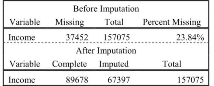
Before Imputation
Variable Missing Total Percent Missing
Income 37452 157075 23.84%
After Imputation
Variable Complete Imputed Total
Income 89678 67397 157075
Table 6. Results of multiple imputation of income with m=20. All 157,075 values of income are now complete.
Results of the imputation are produced in Table 6. Originally 23.84% of incomes were missing, thus the number of imputations m was set to 20 (roughly equivalent to the percentage of missing cases). After imputing 20 possible values of income for each missing individual i at year t, all 157,075 values of income were complete. These 20 values were averaged (excluding any negative values) to form one imputed income for case i,t.
Although imputing 20% of the values for income may seem a potentially serious introduction of error, the multiple imputation documentation suggests that m=20 is not at all unusual. Nevertheless, imputation of income may likely explain why the coefficients on income in the results of the following stages of regression are so puzzling.
B. Construction of Latent measure of Traditionality
1 for comparison, and all other variables are significant at the 0.05, 0.01, and 0.005 significance level.
Figure 13. Model of Traditionality, a latent variable, using five observed gender roles variables. Diagram created in Stata’s SEM builder.
Figure 13 displays the relationship between these variables. We assume Traditionality, the unmeasurable “degree of traditional-mindedness” variable, impacts the women’s responses to each of the five questions asked by the NLSY79. In this way, Traditionality is the explanatory variable and each binary question variable is modeled as depending on the Traditionality quality. Confirmatory factor analysis via SEM allows us to assign values of Traditionality for each women based on the values of the five observed variables.
Table 7 reports the results of the SEM process and Table 8 provides summary statistics for the new variable. The coefficients are as expected: all positive (except wrb_useful),
Measurement Coeff. (Std. Err) Constant P>z
wrb_home 1.000 0.155
(constrained)
wrb_tradition 1.281*** 0.368 0.000
(0.042)
wrb_useful -0.184*** 0.632 0.000
(0.033)
wrb_happy 1.204*** 0.271 0.000
(0.039)
wrb_family 1.004*** 0.226 0.000
(0.034)
Table 7. Results of SEM modeling of latent variable Traditionality according to diagram produced in Figure 13.
Variable Obs. Mean Std. Dev. Min Max
Traditionality 157,075 -0.004 0.067 -0.158 0.477
Table 8. Summary statistics for latent variable Traditionality. The negative mean value suggests that women in this sample tended to be less traditional.
The model is not a perfect fit; the chi-square value is 0.003 whereas an ideal chi-square would be greater than 0.05. However, other goodness of fit measures (see Table 9, appendix) provide a more positive assessment. The root mean square error of approximation is less than 0.05, which indicates a good fit (Browne and Cudeck 1993). The Comparative Fit Index (CFI) and Tucker-Lewis Index (TLI) are both greater than 0.95, and the standardized root mean squared residual is smaller than 0.08 (Hu and Bentler 1999).
After imputing expected income and modeling the latent variable Traditionality, we were able to begin regressions. The results for stage 1, 2, and 3 multinomial logits follow.
C. Stage 1
Multinomial logit with relative risk ratios was used to estimate the causal effect of the probability of being in a certain category.
Of most interest in this stage is the impact of the estimated latent variable Traditionality. The odds of a woman working as a teacher versus not working at all given her Traditionality increases by one unit is 48.12 and significant at the .05 significance level. That is to say, a more traditional woman is expected to prefer working as a teacher rather than not working. All other coefficients on Traditionality are not significant. However, the coefficient representing the odds of a woman working in a professional job given her Traditionality increases also confirms intuition: her odds are 0.5, suggesting that Traditionality negatively impacts the choice of professional and technical occupations.
The relative risk ratio of urban in each occupation category is greater than one,
suggesting that the odds of a woman choosing to work in any occupation rather than not work are greater when she lives in an urban area than when she lives in a rural area. Only the clerical and service work category is significant – which follows intuition, as one would expect much less clerical work opportunities in a predominantly rural area. Age is significant and greater than 1 in all occupations other than teachers, implying that older women are more likely to choose these occupations than to not work. This could be related to the age ranges of the respondents in 1979 – certainly a respondent at age 22 would be more likely to work than a 14 year old
respondent. Education and tenure are both greater than one and very significant (p<0.01) for all occupations, which follows expectations: having more education and working in a job for a longer period of time both increase the odds of choosing an occupation rather than not working.
unemployed. Compared to Hispanic women, both black and non-Hispanic non-black women are much more likely to choose managerial roles than to not work.
The most glaringly unexpected result from this initial regression is the relative risk ratio of income. A coefficient of 0.999 (significant at p=0.01) would be interpreted as women with higher incomes being less likely to choose each occupation than they would be to not work. This goes against the expectation that a woman who sees a higher income potential from a certain occupation category would choose such an occupation rather than not working. However, I believe this can be explained by the inherent reverse causality between occupation and income. In this case, the coefficient suggests that women who already had high incomes might be more likely to not work than to choose an occupation, ostensibly because they do not need the extra income. This suggests that the measures to control for this reverse causality were not altogether successful; therefore I am not confident in the significance of these income coefficients.
D. Stage 2
The results from multinomial logit estimation of the stage 2 cross-sectional occupation choice equation are shown in Tables 11 and 12 in the appendix. This stage represents the
respondent at another moment in her life – when she has had her first child and is either married or in a cohabiting relationship. The base occupation category chosen for comparison remains “home-producers.” Multinomial logit with relative risk ratios was run to estimate the causal effect of the probability of being in a certain category.
she gave birth to her first child is presented in Table 12. The models more or less agree, with some exceptions.
Traditionality continues to follow expectations and stage 1 results. The odds of a woman choosing a professional, managerial, clerical, or education position rather than choosing to not work are lower when women are highly traditional. Effectively, this suggests that women who are highly tradition are more inclined to not work. The relative risk ratio is significant for professionals in both regressions, and the 2-year lag adds significance to managerial, clerical, and teacher categories.
Several variables have strongly positive and significant coefficients, suggesting that they increase the likelihood of a woman choosing any occupation over not working. One such
variable is tenure; the lagged regression further augments the RRRs from around 7 to around 44. A woman who has spent more years with her previous job before children is more likely to choose to work in any of the occupations rather than not working. Education is also significant and largest for the teacher category; this too follows intuition, as the odds a woman choosing to work increase with the years she dedicates to school.
Income continues to produce unexpected results, but slightly less so than in stage 1. The coefficients are significant at the 99% confidence level and equal to 1, suggesting that the
probability that the woman chooses the occupation given her expected income level is equivalent to the probability that she does not work given her income level. That is, income does not
The relative risk ratio is significant for status for both managerial and clerical
occupations with no birth year lag, but the significance drops away after the two year birth lag. Compared to women who are married, cohabiting women are more likely to choose manager or clerical/service positions than to not work.
Prior occupations do not always have a significant odds ratio, but in some cases it is very significant. Women whose prior occupation was in clerical/service or health technicians, for example, are highly unlikely to choose managerial work over staying at home. Women who were previously not employed are also highly unlikely to choose employment after having children (this value is significant for all occupation categories but managers and teachers). The two-year lag adds significance to managers but removes it from health technicians.
E. Stage 3
The results from multinomial logit estimation (using generalized SEM) of the stage 3 panel occupation choice equation are shown in Table 13. Relative risk ratio is not an option provided by gSEM, but robust standard errors were used.
explanation could be women who struggled to conceive and who might hope to have more children, but realistically are not able to.
This model follows the trend of the previous stages in many respects. Despite choosing a different base category for comparison (the managers and supervisors category), tenure,
education, race, and other control variables continue to confirm expectations. For example, more years of tenure at a job has a negative impact on women choosing to stay at home rather than work in a managerial role. This impact is significant at the 99% confidence level. The effect of income continues to hover around 0, defying prior research and intuition. Compared to married women, cohabiting women are less likely choose staying at home or teaching rather than a managerial role (significant at the 99% and 95% confidence levels, respectively).
Implementing the panel data and instruments for presence of first child seems to have had the largest effect on the prior occupation coefficients, which are now almost all significant. The positive coefficients seem to imply that a woman whose prior occupation was, for example, a teacher, is more likely to choose any occupation category rather than become a manager.
The variable of utmost interest is the indicator of the presence of the first child, and the signs on the coefficients confirm this paper’s initial hypothesis: women who have children are more likely to choose clerical/service work, teaching, work as a health technician, or staying at home rather than managing or supervising, and less likely to work as professionals than as managers. Only the coefficient on home-producers is significant (at the 99% confidence level), which makes sense as that is the story often told. Women who previously worked in a
F. Transition Probabilities
The transition probability matrix in Table 14 shows the probability of a woman in one occupation category 2 years prior to giving birth transitioning to one of the seven occupation categories 2 years after giving birth to her first child.
Respondent's occupation
Respondent's occupation
Managers and
Supervisors Professional and Technical Clerical and Service Teacher Health Technician Other Home-Producer Total Managers and Supervisors 25.84% 14.04% 28.65% 1.12% 1.12% 10.67% 18.54% 100.00% Professional and Technical 9.48% 45.97% 19.43% 4.27% 1.90% 6.64% 12.32% 100.00%
Clerical and Service 4.58% 4.95% 52.36% 2.18% 1.60% 11.13% 23.20% 100.00%
Teacher 3.92% 2.94% 8.82% 58.82% 0.00% 6.86% 18.63% 100.00%
Health Technician 2.17% 11.96% 21.74% 1.09% 55.43% 1.09% 6.52% 100.00%
Other 6.10% 3.99% 31.46% 2.11% 0.00% 32.39% 23.94% 100.00%
Home-Producer 2.54% 1.06% 32.59% 1.16% 0.53% 10.58% 51.53% 100.00%
Total 5.56% 6.94% 38.54% 3.66% 2.52% 12.98% 29.80% 100.00%
Table 14. Transition probability matrix. Transition from respondent’s occupation 2 years prior to giving birth to respondent’s occupation 2 years following childbirth.
Percentages along the diagonal correspond the likelihood of returning to the same
occupation after having children. This probability is fairly high for all occupation categories, but lowest for managers and supervisors. The relatively high probability demonstrates the rigidity of the labor market – once a woman has chosen one occupation, there are barriers to switching. There is a fairly high likelihood of switching down, as well. Those previously in clerical and service work have a 23% chance of deciding to remain at home after having children.
SECTION VI:CONCLUSION
What changes when women have children? Are their occupation choices affected by the introduction of a child into their household? My research began with these questions and hypothesized that women make different occupation choices when children are present in their households. Considering the contribution of job attributes such as flexibility to the utility gained from choosing a certain job, I theorized that children, by changing the importance of these attributes, impact the occupational utility function. This changes which occupation provides a woman with the greatest utility. Modeling the decision in a utility-maximizing framework allows us to see how the demographics, market restrictions, individual preferences, and presence of children might theoretically impact the mother’s decision between occupations.
Using data from the National Longitudinal Survey of Youth (1979), this paper has shown that there is a change in how women approach their occupation decision when children are present. In particular, women who have children are indeed more likely to stay at home or work as a teacher than to choose a managing/supervisory occupation, as hypothesized.
birth two years prior do not find much difference in the occupation choice, suggesting that the lag time between childbirth and the return to the workforce is less important than originally expected.
Further research in this area could remove the assumption of exogenous spousal income, allowing for both the mother’s and father’s job choices to vary simultaneously. Furthermore, investigations would do well to seek out better proxies for the expected future wage rate. In endeavoring to simultaneously model labor supply, occupation, and childbirth decision, this paper discovered why such a task has rarely been attempted before. The interrelatedness of the key variables makes for a complicated model which mirrors the complexity of the decision it attempts to capture.
The main limitation of this study is the failure to correctly specify a measure of expected wage without introducing significant error and resulting in an unintuitive impact of predicted wage rate on occupation choice. Access to more data, such as regional labor market fluctuations, might have provided a better instrument and reduced error. Other limitations of the study include the definition of occupation categories, which is subject to human error due to the many varying Census Bureau specifications. As occupation choice has been seen to vary with time and
changing societal expectations, I advise caution when extrapolating to different time periods or countries, which may have significantly different societal views on women working.
APPENDIX
Name in Stata Variable Description
age Age Ranging from 14 to 56
age_start Age at Survey Start Survey began in 1979
age2 Age2 Age squared
child_2lag Lag of Child Born Indicator if first child was born 2 years before or after survey year child_total Total Children Total number of children in 2012
child1 First Child Born Indicator if first child was born in survey year dob_child1 First Child Birth Year Date of birth of the birth of the respondent's first child
id Respondent ID Unique identifier
inc Wage Rate In US dollars
inc_s Spouse Wage Rate In US dollars
jc_autonomy Autonomy Provided by Job Available 79, 82
jc_boss Sex of Supervisor Available 79, 82
jc_coworkers Number of Coworkers at Job Available 79, 82 jc_feedback Provision of Feedback at Job Available 79, 82 jc_females Number of Females at Job Available 79, 82 jc_friend Ease of Developing Friendships at Job Available 79, 82 jc_people Opportunity to Deal with People Available 79, 82 jc_significant Significance of Job Available 79, 82 jc_tasks Ease of Completing the Task at Job Available 79, 82 jc_variety Variety Offered by Job Available 79, 82
married Marital Status Never married, married, separated, divorced, or widowed num_desired Desired Family Size Number of children in respondent's desired family num_expected Number of Children Expected How many more children respondent wants to have num_ideal Ideal Family Size Number of children in an ideal family
occ_5yrs Occupation in 5 years Available 79-84
occ_age35 Occupation at Age 35 Available 79-84
occ_prior Prior Occupation Occupation category in previous survey year occ_r Occupation Category See Table 4 for definitions of categories
partner Partner None, spouse, partner, or other
race Race Hispanic, black, or other
region Region Northeast, north central, south, or west
schyrs Education Years of schooling
sex Sex Female or male; all males were dropped from sample
status Type of Relationship Married or cohabiting
ten Tenure Time spent with current employer, in months
ten_y Tenure Time spent with current employer, in years
urban Urbanization Urban or rural
work_age35 Work at Age 35 Expect to work or be at home? (available 79-84) wr_family Wife Has No Time for Employment Strongly disagree, disagree, agree, or strongly agree (available 79, 82, 87, 04) wr_happy Women Happier to Stay at Home Strongly disagree, disagree, agree, or strongly agree (available 79, 82, 87, 04) wr_home Women's Place is in the Home Strongly disagree, disagree, agree, or strongly agree (available 79, 82, 87, 04) wr_inflation Inflation Necessitates Employment Strongly disagree, disagree, agree, or strongly agree (available 79, 82, 87, 04) wr_tradition Better for Woman to Stay at Home Strongly disagree, disagree, agree, or strongly agree (available 79, 82, 87, 04) wr_useful Wife Feels Useful Working Strongly disagree, disagree, agree, or strongly agree (available 79, 82, 87, 04) wrb_family Wife Has No Time for Employment Disagree or Agree (available 79, 82, 87, 04) wrb_happy Women Happier to Stay at Home Disagree or Agree (available 79, 82, 87, 04) wrb_home Women's Place is in the Home Disagree or Agree (available 79, 82, 87, 04) wrb_inflation Inflation Necessitates Employment Disagree or Agree (available 79, 82, 87, 04) wrb_tradition Better for Woman to Stay at Home Disagree or Agree (available 79, 82, 87, 04) wrb_useful Wife Feels Useful Working Disagree or Agree (available 79, 82, 87, 04)