Where Do the Roads Go?
Evaluating the Impact of Corruption on Infrastructure Allocation in China By: Zhiyi Joycelyn Su
Honors Thesis Economics Department
The University of North Carolina at Chapel Hill
April 2016
Approved:
Abstract
Acknowledgments
I give my sincerest thanks to my advisors, Dr. Simon Alder and Dr. Toan Phan, for their knowledge and guidance throughout this entire year of the research process. Even though I came into the process completely clueless, they have both been the most understanding and
I. Introduction
One of the biggest dangers of corruption, as evident in economics literature, is it produces inefficient market outcomes (Mauro 1995, 1997, Rose-Ackerman 1997, Bó & Rossi 2007). Economic inefficiency can occur when government officials offer undue benefits to companies that offer monetary or non-monetary bribes and kickbacks, resulting in a sub-optimal allocation of resources. Where winners are not decided based on competition, this leads to lower quality products and higher costs of production (Bai & Qian 2010). The inefficient allocation of resources can have a geographical dimension as well. Political pressures and informal personal influences can result in regional favoritism, skewing the geographical distribution of public resources to areas that yield greater political benefits than economic efficiency. In democratic governments, this process is commonly understood as pork-barrel politics where government officials provide selective benefits to their constituents in order to garner votes. Intuitively, authoritarian regimes, though they lack democratic electoral processes, should observe a similar yet even stronger effect of skewed public resource distribution as a result of inadequate checks and balances within the political system (Hodler & Raschky 2014). This paper examines the presence of regional favoritism in an autocratic regime — China — focusing specifically on the geographical distribution of paved roads as determined by the birthplaces of powerful
governmental officials.
China, corruption is especially rampant in sectors like transportation where large-scale
infrastructure projects allow funds to be maneuvered around more easily. Inefficient allocation of resources impedes China’s economic growth and lowers the rate of returns on infrastructure investment (Tanzi and Davoodi 1997). In a country where infrastructure investment composes around ten percent of its annual economic output, corruption poses a significant threat to the domestic economy (Dobbs et al. 2013).
Surprisingly, little empirical work has been conducted evaluating the impact of corruption in China’s infrastructure investment. This is in part due to the hidden nature of the corruption and the lack of effective tools of measurement and evaluation (Guo 2008). The
question of this study is as follows: can one observe corruption, in the form of regional favoritism, in the distribution of public resources in China?
This paper answers the question by examining the impact of high-level government officials on the geographical distribution of public infrastructure to their hometowns in China. More specifically, it uses panel data to explore variation across different prefectural-level cities in China from 1993 to 2009. I focus on the geographical distribution of paved roads in particular, controlling for factors that may influence the area of paved roads in the city such as the size of the population, the size of the city, and the overall income level of the city. I hypothesize that the top-down selection process of government officials implies that lower-level officials take on the preferences of their superiors and direct their resources in ways that will benefit their superiors or those who got them in power. To increase his or her chance for promotion and obtain favor from his superior, the lower-level official will build more roads in the birthplaces of the national-level officials. I find that on average, high-national-level government officials in China do have a positive effect on the area of paved roads in their hometowns, even after controlling for time-invariant prefectural-level city characteristics through fixed effects. In addition, I find that the prevalence of hometown favoritism increases as the officials’ years in office increase.
research studies look at the same phenomenon in authoritarian regimes (Golden & Min 2013). My work contributes to the general strand of literature on distributive politics and more importantly, the sub-strand that focuses on distributive politics in autocratic states.
The rest of this paper is organized as follows: Section II provides a brief overview of related literature on corruption in China and distributive politics. Section III describes the background of public office selection and promotion and infrastructure investment in China. Section IV develops the theoretical framework behind this study by borrowing core concepts from Do et al.’s study on distributive politics. Section V and VI present the empirical framework and the data that I use for this paper. Section VII provides a discussion of the findings and Section VIII, the conclusion.
II. Related Literature
A. Corruption
Scholars have addressed corruption’s impact on growth and its effect on the composition of public expenditures (Mauro 1995; Mauro 1998). In one of the seminal pieces of literature on corruption, Paolo Mauro (1995) found a significant negative relationship between corruption and growth rates across a host of countries. Mauro also found that corruption, which he defines as the degree to which business transactions involve questionable payments, not only lowers growth rates but it also lowers private investment. Cole et al’s study that analyzes the distribution of foreign direct investment (FDI) in China found that FDI is attracted to provinces with higher level of government efficiency and are actively involved in the fight against corruption (Cole et al. 2008, 1494). Further, corruption is widely understood to be more prevalent in the
infrastructure sector (Wade 1982, Rose-Ackerman 1996). It can reduce growth by increasing unproductive public investment that yields low returns (Devarajan et al. 1996, Tanzi and Davoodi 1997) and reduce the quality of infrastructure (Tanzi and Davoodi 1997).
As I discussed briefly in the introduction section and as evident through these studies, the perception of high-level corruption in China has significant impact on all levels of economic activity and may be detrimental to the growth of the Chinese economy. In a country where economic growth provides the legitimacy of the ruling party, corruption in China is highly destabilizing to both its economic and political systems. The problem may manifest itself
through many channels, i.e. bribery, embezzlement and etc., but less well known are the informal influences that create the same economic inefficiencies. This study contributes to an expanded understanding of corruption and specifically explores the effect of political leaders on the unequal distribution of resources.
Harold Laswell (1936) infamously wrote that politics is about “who gets what, when, how;” it is the authoritative allocation of resources (Su & Yang 2000). In democratic regimes, government officials are responsible to their constituents. They are assumed to be office seeking and their performance is evaluated by domestic constituents who have the ability to take the officials out of office. Pork-barrel politics (Ferejohn 1974), the practice of allocating greater number of resources to domestic constituents in order to secure votes of gain reelection, is a widespread practice in the United States and in other democracies. Albouy (2009) finds that states represented by members of Congress in the majority party receive greater federal grants,
especially in transportation and defense spending. Alternatively, Berry et al. (2010) posit that the president is the one who has the authority to decide where to allocate federal funds. They found that districts and counties receive significantly more funding when their representing members of Congress belong to the same party as the president. While the studies discover differing results, they show that powerful government officials do affect the ways in which federal funds are geographically distributed.
Hodler and Raschky (2014)’s research looked at the light intensities of political leaders’ hometowns in all countries with more than half a million inhabitants and found them to be
significantly more than the light intensities of regions that are not also the hometowns of political leaders. They conclude that regional favoritism is a widespread phenomenon that is more
prevalent in autocratic countries.
In autocratic countries, domestic constituents do not elect officials into office. Instead, officials gain support from their superiors who have the power to elect them into office (Do et al. 2013). In China, economic achievements are used to impress superiors in hopes of being
rewarded with promotion. How does this elite selection dynamic affect distributive politics in autocratic regimes? Little empirical research have been done on this topic, but the only one and possibly the closest study to my paper looks at hometown favoritism in Vietnam (Do et al. 2014). The authors found that differing levels of government officials are able to influence the budget allocation process once promoted and greater levels of infrastructure are observed in their hometowns. My results are consistent to that of Do et al’s, but my paper differs by showing an increasing impact of high-level officials on public resource allocation over time, not simply after promotion to higher-level office. My paper contributes to the void in the economics literature on distributive politics in autocratic countries and focuses on the case study of China. In the next section, I briefly describe the basic mechanisms of political selection and the fiscal process in China before I introduce my theoretical framework.
III. Background on China A. Political Selection in China
2000). Jia et al. (2015) also shows that a politician’s connections with top leaders in the Chinese Communist Party also increase the chances of promotion. More formally, however, the selection of officials in China is determined based on the nomenklatura system:
The nomenklatura…consists of lists of leading positions over which party units exercise the power of appointment and dismissal, lists of reserve candidates for those positions, and rules governing the actual processes of appointments and dismissals… Through this vehicle the party monopolizes the power to determine who will join — and who will be forced out of — the country’s elite in all spheres (Lieberthal 1995, 209).
Since 1984, the Party has practiced the “one rank down” appointment where an official’s chances of promotion were almost entirely dependent on the support of his immediate superior. This, in turn, has increased the possibility of local despotism (Lieberthal 1995, 212). The immense promotional power given to each official’s superior would also create incentives for corrupted practices among the all ranks of the political system in order to gain upward political mobility.
B. Chinese Fiscal Process
The budgetary process was highly centralized in China until the onset of market reforms in the 1970s. The hierarchy of the Chinese political system starts at the top with national, to provincial, prefectural, county and finally township-level. Because of fiscal decline in China, the
“The cessation of administrative approval over non-public investment was widely interpreted by subnational governments to mean that only projects funded by the budget were required to go through the institutional framework. The vast majority of public investment was considered “exempted” from 2004 onward (Wong 2014, 16).” Because of the devolution of China’s budgetary process, local officials have a greater amount of authority in making decisions on infrastructure.
Guo (2009) argues that local Chinese officials both have the incentives and the capacity to influence local budgets. Related to the political selection process in China, local officials often build large-scale development projects that are highly visible and quantifiable, like roads,
highways, and other large infrastructure projects in order to impress their superiors. They are able to do so as a result of the decentralization of budgetary control. Chinese local officials nowadays assume “an unprecedented large proportion of government spending responsibilities and day-to-day control over various economic activities (Guo 2009, 625).” As a result of local governments’ increased autonomy, while the Central Government continues to outline goals for infrastructure development every five years through the Five-Year Plans, local government officials are able to exercise discretion over where roads are built as long as they reach the identified goals.
IV. Theoretical Framework
Local-level government officials, as the primary economic agents, are defined in this study as officials at the prefectural level. It is based on the assumption that officials at lower-levels will always seek to impress their superiors at the next level higher because of the “one rank down” practice of political appointment. To illustrate, a village level official will seek to impress a county level official, who is trying to impress a prefectural level official. Because of these layers of political pleasing, lower-level officials can be considered to have similar preferences as they eventually align with the preferences of national-level officials.
Local level officials face a decision to allocate roads to the birthplaces of national level officials as opposed to otherwise. The reasoning is that a local official can secure the national-level official’s favor by allocating the local government’s budget for roads to the hometown of a national-level official. It is based on the assumption that better infrastructure yields greater social utility for a city. Since a national official will have an existing social network in his birthplace, the local official may want to influence the allocation of infrastructure to benefit the national official’s social network in order to obtain favor from him/her, increasing his chances of promotion.
Local officials benefit from allocating roads to the national-level officials’ hometowns because by building roads in the hometowns of national-level officials, these local officials gain favor from the national-level officials and increase their chance of promotion within the Party system. The assumption is that the Chinese political system is similar to a single internal labor market without outside options and officials have great incentive to remain in office (Li and Zhou 2004).
prefecture, county, township, and village. While infrastructure can also be funded by
international organizations’ loans and foreign capital (Démurger 2000), these other sources of funding remain a small portion of total funding (Bai & Qian 2009). Thus, local officials do not have an indefinite amount of resources to spend on allocating roads to national officials’ birthplaces, which creates a scenario where the local officials have to determine the costs and benefits and allocate an amount based on his expected benefits.
Therefore, a local level official is modeled in a simple two-period discounted utility as follows:
𝑉! =𝑢!+β Ε 𝑢!
=𝑢! +β(𝑃𝑢! + 1−𝑃 𝑢!); (a)
where β is a positive constant
The total utility of a local official, with respect to roads, is the utility that he receives in the current period as a local official (𝑢!) plus the utility that he expects to get in the second period Ε 𝑢! at a discounted rate (β). The utility that a local official gets in the second period is
dependent on the probability (P) that he gets promoted. In a simplistic world where there are only two goods, the official can decide to use his budget (𝐵) on either allocating roads to a higher-level official’s birthplace (𝑐𝑅) or on anything else that he personally prefers. Since
building roads in a higher-level official’s birthplace does not directly benefit himself, these roads are modeled as a total cost (𝑐𝑅) out of his budget 𝐵, where 𝑐 is the per unit cost of roads. His utility in the current period is therefore a function of1:
1𝑢
𝑢! = 𝑓(𝐵,𝑐𝑅) ; (b)
where 𝐵 and 𝑐 are positive constants and 𝑢!
!(𝑅) <0
Further, in this simple scenario, the probability of promotion can be written as a function of the cost of roads and the local official’s budget. This time, however, the amount of money that the local official allocates to building roads in a high-level official’s birthplace (𝑐𝑅) out of his budget 𝐵 increases his chance for promotion:
P= 𝑔(𝐵,𝑐𝑅) ; (c)
where 𝐵 and 𝑐 are positive constants and P′(𝑅) >0
Substituting these two functions into 𝑢! and P, the local official’s total utility becomes: 𝑉! =𝑢!+β(𝑃𝑢!+ 1−𝑃 𝑢!)
= 𝑓(𝐵,𝑐𝑅)+β(𝑔(𝐵,𝑐𝑅)𝑢! + 1−𝑔(𝐵,𝑐𝑅) 𝑓(𝐵,𝑐𝑅)); (d)
where 𝑓 is a decreasing function and g is an increasing function
Maximizing this function with respect to 𝑅 yields a unique solution for the optimal amount of roads that would be allocated in higher-level official’s birthplace. The tradeoff is that building more roads in a higher-level official’s birthplace decreases the local official’s utility in the current period but increases his chances for promotion and therefore his expected utility in the next period. As such, the more a local official cares about being promoted, the bigger share of the budget he would allocate to building roads in a higher-official’s hometown.
Based on this theoretical framework, I posit that:
H1: To maximize one’s chances for promotion, a local official who has budgetary control
H2: The area of paved roads will increase as the number of high-level officials increases
in cities that are also the birthplaces of high-level government officials, ceteris paribus. V. Data
This study utilizes a panel dataset that draws from data on officials’ career and data on China’s annual statistics from 1993 to 2009 with prefecture-level cities as the unit of
observation.
A. China’s Annual Statistics
the missing data for those two years, there remains 15 years of observations for most of the cities, which will be sufficient for the purpose of this research study.
Although there are reasons to question the reliability of the data from China Statistical Yearbooks, there are no clear alternatives for other sources of data that I could retrieve. Since I am analyzing data on a large number of cities, I assume that if data were unreliable or inflated, they would be normalized across all cities.
B. Career Data
The other major data source on officials’ career data comes from China Vitae, a non-profit organization based in Maryland, United States that was founded in 2001 to collect information on China’s top leadership. The organization runs a website that provides career information of Chinese government officials to the public. I use the dataset that Jia et al. (2015) constructed from China Vitae in their study on the impact of social networks on political selection in China. The dataset includes all of the provincial governors, provincial secretaries, and politburo
members who have held office for at least twelve months in between June 1993 and June 2009. A total of 187 officials whose curriculum vitaes were found on China Vitae are included and they are the high-level officials to whom I refer in this study. These CVs include the official’s name, province of birth, year of birth, and the important positions that they held. Additionally, I
obtained the corresponding birthplaces for each of the 187 officials from China Vitae. Because many
of officials’ birthplaces were listed at an administrative level lower than the prefecture-level, I then
matched the birthplaces with corresponding prefectural-level cities.
C. Key Independent Variable: Official
In order to evaluate the impact of officials on the area of paved roads in each city across 17 years, I
combined the two datasets into one panel dataset grouped by prefecture-level cities. I constructed the
first took a count of the number of officials who were provincial secretaries, provincial governors, or
politburo members in each year by each prefecture. Then I took the cumulative sum of the number of
national officials from 1993 to 2009. To illustrate, if there were two officials in office in Ankang in
1993 and three officials in office in the same city 1994, the value under the official variable in 1994
is the cumulative sum of officials from 1993 and 1994, which equals to 5 officials. The formal
definition of the official variable is as follows:
𝑜𝑓𝑓𝑖𝑐𝑖𝑎𝑙!,! = !""#! !𝐼𝑛𝑂𝑓𝑓𝑖𝑐𝑒!,! ; (e)
where 𝐼𝑛𝑂𝑓𝑓𝑖𝑐𝑒!,! represents the current number of officials who were born in city i and are
in office at time t-n, where n represents the total number of years since 1993. The 𝑜𝑓𝑓𝑖𝑐𝑖𝑎𝑙!,! variable
represents the cumulative number of official-years who were born in city i and their total years in
office in time t. The logic for taking the cumulative sum of officials as the key independent variable
is because the area of paved roads in each city is a stock variable. The roads that were built in 1993
will be considered in 1994; the impact that an official has on the area of paved roads is
non-reversible. While the 𝑜𝑓𝑓𝑖𝑐𝑖𝑎𝑙!,! variable increases in both the number of officials and their total
years in office, I will call 𝑜𝑓𝑓𝑖𝑐𝑖𝑎𝑙!,! cumulative number of official-years from this point forward for
the sake of simplicity.
The final sample with which I conduct my analysis for this study includes 3,882 observations across 15 years and 276 prefecture-level cities. Table 1 describes the list of key variables used in this study. Even though all other variables had more than 4,400 observations, the variable for the area of paved roads only contains 3,882 observations, and because of this reason it reduces the size of my sample down by around 800 observations.
interest to this study. To differentiate the growth by cities that are also hometowns of high-level officials as opposed to those that are not, Table 2 in the Appendix shows the tremendous positive difference in the growth in roads in cities that are also the birthplaces of high-level officials as opposed to otherwise. The statistic that I obtained from testing the significance of that difference using a t-test was 14.617.
Note: Key variables that are used in this study. The units for each of the variables are as follows: Area of land (km2), real GDP (Million RMB), area of paved roads (km2), population (1,000). The official dummy variable takes on a 0 when a city has never been an official’s birthplace in the years of
observation, and 1 when it has had at least one official born in the city. Construction of the cumulative # of officials variable is explained on the previous page.
Figure 3 to Figure 6 utilize maps to show the distribution of paved roads and government officials across provinces and prefecture-level cities. They provide some visualization for the patterns of correlated growth that are described in this paper. Figure 3 shows the distribution of paved roads in 2009, while Figure 4 shows per capita paved roads in 2009. Figure 5 shows the distribution of the cumulative number of national officials across the country in 2009, while Figure 6 shows the number of national officials per capita. The darker regions as shown on the maps experience higher density of roads or officials, both in nominal terms and in per capita terms.
VI. Empirical Framework
Table 1: Descriptive Statistics (1993-2009)
Variable Obs. Mean Std. dev. Min Max
Year 3,882 2,002 4.777 1993 2009
Prefecture-level Cities 3,882 139 80 1 276
Area of Land 3,882 1,818 2,048 50 20,169
Real GDP 3,882 31,840 56,667 579 896,805
Area of Paved Roads 3,882 6.913 9.519 0 122.8
Population 3,882 1029 882 114 8,014
Official Dummy 3,882 0.313 0.464 0 1
The primary objective for my empirical analysis is to observe whether there is a difference in the area of paved roads in China in prefecture-level cities that are also the birthplaces of national-level officials as opposed to otherwise. I test both the effect of officials and the effect of a one-unit increase in the cumulative number of official-years by estimating them with the following equations:
ln 𝑟𝑜𝑎𝑑𝑠!" =𝛽!+𝛽!𝑜𝑓𝑓𝑑𝑢𝑚!,!!!+𝛾𝛸′!,!!! +𝑢!+ 𝜃!+𝜀!" (f)
ln 𝑟𝑜𝑎𝑑𝑠!" =𝛽!+𝛽!𝑜𝑓𝑓𝑖𝑐𝑖𝑎𝑙!,!!! +𝛾𝛸′!,!!!+𝑢!+ 𝜃!+𝜀!" (g)
where 𝑟𝑜𝑎𝑑𝑠!" is the area of paved roads in each prefectural-level city i at time t, 𝑜𝑓𝑓𝑑𝑢𝑚!,!!! is a dummy variable that takes on the value 0 when the cumulative number of
official-years is zero and the value 1 when the cumulative number of official-years is greater than zero. 𝑜𝑓𝑓𝑖𝑐𝑖𝑎𝑙!"!! is the cumulative number of official-years city i at time t as I explained in
the previous section, 𝛸′!"!!, a vector of control variables that includes 1) the log of real GDP, 2) the log of the size of population, and 3) the log of the area of the city. 𝑢! and 𝜃! are city-specific and time-specific fixed effects, respectively, and 𝜀!" is the error term. I included an s period time
lag in my model for all independent variables to account for the delay in the time between when an official decides to allocate funds for roads construction and when the road has completed construction.
The reason for including the GDP, population size, and city size as my explanatory variables is because I expect an increase in each of these three factors to increase the area of paved roads in a city. The time-invariant error term 𝑢! denotes prefectural-level fixed effects that control for constant prefecture-specific characteristics, such as the geographical location of a city. The time-variant error term 𝜃! denotes year fixed-effects that control for the natural trend
exogenous shocks such as policies that have nation-wide consequences. The remaining error term 𝜀!" denotes an unobserved effect that varies across time and prefectures. This error term is
assumed to be independent from any of the explanatory variables and is normally distributed. Given the model described above, I expect the coefficient of interest 𝛽! in both equations
(f) and (g) to be positive, as it will indicate a positive difference between the area of paved roads in cities that are the birthplaces of high-level government officials and those that are not, all else equals. The interpretation of a positive 𝛽! is that regional favoritism exists in China. 𝛽! is the
constant intercept when all independent variables are zero, which is of little importance in the context of this model. Robust standard errors are used in this model, where I cluster them at the level of prefectures.
To further disaggregate the effect on paved roads at different levels of officials, I
deconstruct the 𝑜𝑓𝑓𝑖𝑐𝑖𝑎𝑙!"!! variable into evenly weighted categories and then test the following
model:
ln 𝑟𝑜𝑎𝑑𝑠!" =𝛽!+𝛽!𝑜𝑓𝑓𝑖𝑐𝑖𝑎𝑙0!,!!!+𝛽!𝑜𝑓𝑓𝑖𝑐𝑖𝑎𝑙1_2!,!!!+𝛽!𝑜𝑓𝑓𝑖𝑐𝑖𝑎𝑙3_4!,!!!+
𝛽!𝑜𝑓𝑓𝑖𝑐𝑖𝑎𝑙5_9!,!!!+𝛽!𝑜𝑓𝑓𝑖𝑐𝑖𝑎𝑙10_36!,!!!+𝛾𝛸′!,!!!+𝑢!+ 𝜃!+𝜀!" (h)
The variable official0 is a category that simply accounts for the cities where no high-level official was born. Cities that were the hometowns of at least one high-level official were then divided into groups of relatively equal sizes. The variable official1_2 is the category that accounts for the cities where one or two high-level official were born, official3_4 for the cities where three or four high-level officials were born, official5_9 for cities with five to nine officials and official10_36 for cities with ten to thirty-six officials. I expect 𝛽! to be zero, as it will
positive difference between the area of paved roads in cities that are also birthplaces of officials compared to otherwise. Given Hypothesis 2, I also expect 𝛽! > 𝛽!> 𝛽! > 𝛽!, which will indicate
that the impact on area of paved roads increases as the cumulative number of official-years increases.
Potential problems may arise in this model. First, the key independent variable official may be endogenous as the total area of paved roads may reflect the competency level of officials and thus lead to a higher number of officials found in national office. Fortunately, as the model prescribes, a time lag in counting the number of officials in national office can help resolve the issue as the area of paved roads in this period cannot retroactively affect the number of officials in national office in the last period.
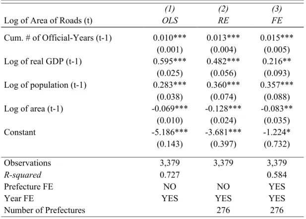
I determine the effect of each explanatory variable described in Equation 1 on the area of paved roads in China from 1993 and 2009 using pooled OLS estimation. I then treat the data as a panel dataset and conducted the regressions using fixed effects and random effects to observe the differences in the coefficients estimated by each model. The results for different methods are reported in Table 4 in the Appendix. The RE and FE models do not reveal many discrepancies in the coefficient estimates. Unsurprisingly, the Hausman test fails to reject the hypothesis that the coefficient estimates are equal, suggesting that the two estimates are sufficiently close and either model could be used in my study. I choose to use the FE model in this study, as it is highly likely that the time invariant error term 𝑢! is not independent from my independent explanatory
variables, thereby yielding more conservative estimates.
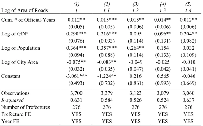
the area of paved roads in each city is most significant when I take a one-year lag or a two-year lag. The magnitude and significance of coefficients are lower in all other periods. Since the one-year lag and two-one-year lag yield similar results, I choose to use a one-one-year lag as my baseline model because lagging the explanatory variables by two years reduces the number of
observations2.
VII. Findings and Discussion
The main results for this study are presented in Table 2. The coefficient of interest in Model (1) is positive but not statistically significant. This suggests that the change from having no level government official who was born in prefecture-level city i to at least one high-level official who was born in city i does not have a significant impact on the area of paved roads in city i. Model (2), however, shows that the area of paved roads increases by 1.5 percent as the cumulative number of official-years increases, all else equals.
While Model (1) and (2)’s results may seem contradictory at first glance, they suggest there is a heterogeneity in how the cumulative number of official-years affect the area of paved roads. To test this, I break the officials variable down into five different count categories. Column (3) in Table 2 reports the results of the regression. The coefficients of interest are the ones corresponding to the various categories, with “No Official” omitted as the baseline category. The coefficients reported on the categories are compared to the baseline cities where no official was born. While the first three categories, “One or Two,” “Three or Four,” and “Five to Nine” do not show significant results, the category “Ten to Thirty-Six” produces a coefficient that is positive and statistically significant at the 95 percentage confidence level. Compared to cities that are not the hometowns of high-level government officials, cities with more than ten
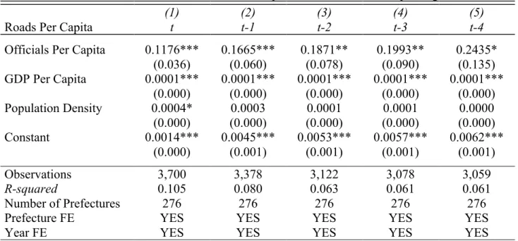
2 Table 6 in the Appendix reports the same regression testing different time periods but with per capita measures.
cumulative officials on average report a 22.3 percent increase in the area of paved roads, all else equals. This seems to suggest that the onset of corruptive practices experience a delay or the presence of multiple leaders have colluding effects.
Table 2: Dynamics of Hometown Favoritism
(1) (2) (3) (4) (5)
Log of Area of Roads lgroad lgroad lgroad lgroad lgroad
Official Dummy 0.059
(0.049)
Cum. # of Official-Years (t-1) 0.015*** 0.011*** 0.005***
(0.005) (0.004) (0.002)
One or Two 0.070
(0.043)
Three or Four 0.031
(0.063)
Five to Nine 0.088
(0.067)
Ten to Thirty-Six 0.223**
(0.093)
Log of GDP (t-1) 0.237** 0.216** 0.228** 0.133** 0.219***
(0.095) (0.093) (0.094) (0.065) (0.053) Log of Population (t-1) 0.351*** 0.357*** 0.357*** 0.223** 0.116**
(0.091) (0.088) (0.089) (0.097) (0.054) Log of Area of City (t-1) -0.083** -0.083** -0.086** -0.053* -0.034**
(0.036) (0.035) (0.035) (0.030) (0.014)
Log of Area of Roads (t-1) 0.287** 0.619***
(0.128) (0.103)
Constant -1.389* -1.224* -1.325* -0.552 -1.743***
(0.752) (0.732) (0.741) (0.518) (0.477)
Observations 3,379 3,379 3,379 3,174 3,174
R-squared 0.581 0.584 0.583 0.611 0.571
Number of prefectures 276 276 276 276 276
Prefecture FE YES YES YES YES NO
Year FE YES YES YES YES YES
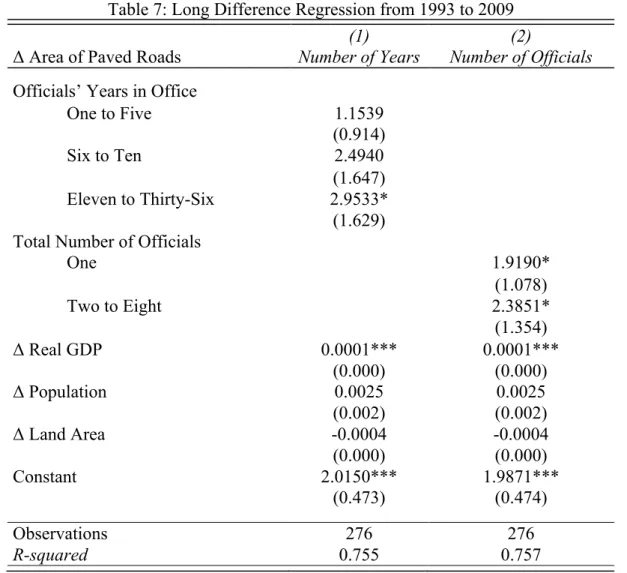
To better understand which is a more important factor in the increase in the area of paved roads, the number of years an official is in office or the number of officials, I analyze the official variable in greater detail. The value given by the official variable in the last year of observation, 2009, gives the total number of years in which a city has had high-level officials in office. I create a separate variable that counts the total number of officials in office in each city from 1993 to 2009. I then regress the two variables, one that accounts for the total number of years in office the other that accounts of the total number of officials, on the total area of paved roads in each city. Taking the long difference in each variable between 1993 and 2009 essentially reduces the panel into a cross-sectional dataset, so I conducted my analysis using the OLS multiple regression method. The results are reported in Table 7 in the Appendix and they suggest that both the number of years a high-level official is in office and the number of high-level officials contribute to the positive difference in the area of paved roads. The effect on paved roads is greater as both the number of years increases and the number of high-level officials increases.
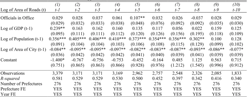
How many years after a high-level official is in office will his or her hometown observe an increased area of paved roads? To explore this question, I tested several lags on the dummy variable that indicates when one or more officials from city i are currently in office in time t. The results are reported in Table 8, where all indicators for the periods that I tested were insignificant except for the indicator during time t-5. This can be interpreted as the presence of one or more high-level official five years ago has a significant positive impact on the amount of paved roads in his or her hometown today. This finding is consistent with Hodler and Raschky’s study where they found that political leaders “take a few years before they successfully engage in regional
I strengthen the robustness of my findings by taking the lag of the dependent variable, log of area of roads, as an independent variable on the right hand side in order to reduce the
existence of autocorrelation in my baseline model. The results are reported in Column (4) in Table 2. While “Log of Area of Roads” in time t-1 is positive and statistically significant, the coefficient for “Cum. # of Officials” also remained positive and statistically significant, though it dropped down from the original baseline model estimate of 0.015 to 0.009. As Hodler and
Raschky (2014) did in addressing the Nickell (1981) bias in their study, I follow Angrist and Pishke (2009)’s recommended method of estimating a specification with fixed effects (but no lagged dependent variable) and one with the lagged dependent variable (but no fixed effects). The true effect should lie between the estimates of the two specifications (Hodler & Raschky 2014, 1011). Column 5 in Table 2 reports the results of the specification that estimates the lagged dependent variable (but does not include fixed effects). The coefficient estimate has decreased in magnitude but remains positive and significant. This suggests that the true effect of a unit
increase in cumulative number of official-years on the area of paved roads lies in the positive range and is statistically significant.
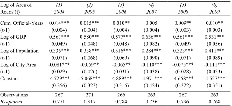
official variable is significant from 1993 to 2003, and all but one of the coefficient estimates become significant beginning in 2004 when the reforms took effect.
The sudden change in the impact of high-level officials on roads construction may be because engaging in corruptive behaviors in the form of regional favoritism had become easier and less costly. Infrastructure projects no longer needed to undergo long process of approvals from the Central government – they can now be decided on the end of local officials. As a result of greater autonomy, corruption grows rampant. The findings for yearly cross-sectional analysis support the theoretical framework laid out in the previous sections. When local officials are given greater amount of autonomy, the results show that they build more roads in the birthplaces of high-level officials. The results support this paper’s argument that local officials build more roads in the hometowns of national-level officials in order to obtain favor from their superiors and increase their chances of promotion.
VIII. Conclusion
Where do the roads go in China? This study has shown that on average, more roads are
built in cities that are the hometowns of high-level officials, suggesting corruption in the form of
regional favoritism. While the national-level officials themselves may not have direct budgetary
powers to control where roads are built, the top-down selection of government officials create
incentives for lower-level officials to build roads in the hometowns of their superiors in order to
increase their chances of promotion. I demonstrate empirically the positive difference in the area
of roads in cities that are also birthplaces of national-level officials by using a panel on Chinese
prefecture-level cities from 1993 to 2009. The findings are subjected an interesting nuance: not
only does it take time before officials engage in regional favoritism, the effect increases as the
This paper also shows that the 2004 reform in public investment management
exacerbated the impact high-levels officials could have on roads construction. It created
incentives for officials to engage in corruptive behaviors by reducing oversight and hence, the
risk of getting caught. Thus, while decentralization of the fiscal process is evidence of a more
efficient government, the tradeoff is the economic efficiency that was given up as a result of
corruptive behaviors. Creating new policies to increase oversight and not bureaucracy is much
needed if China were to strive for an efficient government.
While the focus of this study is China, the same empirical results would likely be present
in other autocratic countries and in other forms of public investments, such as electricity
coverage, Internet coverage, and water infrastructure. Corruption can sometimes be not at all
obvious when it relies on channels of informal influences and social networks, and regional
favoritism, as a form of corruption, may not necessarily yield negative results. Thus, a greater
body of research should be dedicated to uncovering these disguised forms of corruption in order
to gain a better understanding of the problem. While the findings of this study reveal the effect of
high-level officials on roads construction, they do not show if the allocation of roads to officials’
hometowns is truly inefficient. This is a topic that requires further research as it will help
References
Ackerman, Susan. Corruption and Government: Causes, Consequences, and Reform. New York:
Cambridge University Press, 1999.
Albouy, David. "Partisan Representation in Congress and the Geographic Distribution of Federal
Funds." National Bureau of Economic Research, 2012.
Alder, Simon, Lin Shao, and Fabrizio Zilibotti. "Economic Reforms and Industrial Policy in a Panel of Chinese Cities." SSRN Electronic Journal SSRN Journal, May 2015.
https://sites.google.com/site/simonalderch/research.
Angrist, Joshua David, and Jörn-Steffen Pischke. Mostly Harmless Econometrics: An Empiricist's Companion. Princeton: Princeton University Press, 2009.
Bai, Chong-En, and Yingyi Qian. "Infrastructure Development in China: The Cases of
Electricity, Highways, and Railways." Journal of Comparative Economics, 2009, 34-51.
Berry, Christopher R., Barry C. Burden, and William G. Howell. "The President and the
Distribution of Federal Spending." American Political Science Review, 2010, 783-99.
Bó, Ernesto Dal, and Martín A. Rossi. "Corruption and Inefficiency: Theory and Evidence from Electric Utilities." Journal of Public Economics 91, no. 5-6 (2007): 939-62.
Bo, Zhiyue. "Economic Performance and Political Mobility: Chinese Provincial Leaders." Journal of Contemporary China 5, no. 12 (1996): 135-54.
Castells, Antoni, and Albert Solé-Ollé. "The Regional Allocation of Infrastructure Investment:
The Role of Equity, Efficiency and Political Factors." European Economic Review, 2003,
1165-205.
Cole, Matthew A., Robert J.r. Elliott, and Jing Zhang. "Corruption, Governance and FDI
Location in China: A Province-Level Analysis." Journal of Development Studies, 2008,
1494-512.
Dobbs, Richard et al., “Infrastructure Productivity: How to Save $1 Trillion a Year.” McKinsey
Global Institute, 2013.
Démurger, Sylvie. "Infrastructure Development and Economic Growth: An Explanation for
Regional Disparities in China?" Journal of Comparative Economics, 2000, 95-117.
Devarajan, Shantayanan, Vitaya Swaroop, and Heng-fu Zou. "The Composition of Public
Expenditure and Economic Growth." Journal of Monetary Economics 37, no. 2-3 (1996): 313-44.
Do, Quoc-Anh, Kieu-Trang Nguyen, and Anh Tran. "One Mandarin Benefits the Whole Clan:
Hometown Infrastructure and Nepotism in an Autocracy." SSRN Electronic Journal
SSRN Journal, 2013. Working Paper.
Franck, Raphaël, and Ilia Rainer. "Does the Leader's Ethnicity Matter? Ethnic Favoritism, Education, and Health in Sub-Saharan Africa." American Political Science Review 106, no. 02 (2012): 294-325.
Golden, Miriam, and Brian Min. "Distributive Politics Around the World." Annual Review of
Political Science. 2013, 73-99.
Golden, Miriam A., and Lucio Picci. "Proposal For A New Measure Of Corruption, Illustrated
With Italian Data." Economics & Politics Economics and Politics, 2005, 37-75.
Guo, Gang. "China's Local Political Budget Cycles." American Journal of Political Science,
Guo, Yong. "Corruption in Transitional China: An Empirical Analysis." The China Quarterly
CQY, no. 194 (2008): 349-64.
Hodler, Roland, and Paul A. Raschky. "Regional Favoritism." The Quarterly Journal of Economics 129, no. 2 (2014): 995-1033.
Jia, Ruixue, Masayuki Kudamatsu, and David Seim. "Political Selection In China: The
Complementary Roles Of Connections And Performance." Journal of the European
Economic Association, 2015, 631-68.
Kramon, Eric, and Daniel N. Posner. "Who Benefits from Distributive Politics? How the
Outcome One Studies Affects the Answer One Gets." Perspectives on Politics 11, no. 02 (2013): 461-74.
Li, Hongbin, and Li-An Zhou. "Political Turnover and Economic Performance: The Incentive
Role of Personnel Control in China." Journal of Public Economics, 2004, 1743-762.
Lieberthal, Kenneth. Governing China: From Revolution through Reform. New York: W.W. Norton, 1995.
Maskin, Eric, Yingyi Qian, and Chenggang Xu. “Incentives, Information, and Organizational
Form.” Review of Economic Studies, 2000, 67(2): 359–378.
Mauro, P. "Corruption and Growth." The Quarterly Journal of Economics, 1995, 681-712.
——— "Corruption and the Composition of Government Expenditure." Journal of Public
Economics, 1998, 263-79.
Nickell, Stephen. "Biases in Dynamic Models with Fixed Effects." Econometrica 49, no. 6
(1981): 1417-426.
Rose-Ackerman, Susan. “Corruption, Inefficiency, and Economic Growth” Nordic Journal of Political Economy, 1997, 3-20.
——— “When is Corruption Harmful?” 1997 World Development Report, 1996. Background
paper.
Su, Fubing, and Dali L. Yang. "Political Institutions, Provincial Interests, and Resource
Allocation in Reformist China." Journal of Contemporary China, 2000, 215-30
Tanzi, Vito, and Hamid Davoodi. "Corruption, Public Investment, and Growth." The Welfare State, Public Investment, and Growth, 1998, 41-60.
Treisman, Daniel. "The Causes of Corruption: A Cross-National Study." Journal of Public
Economics, 1998, 399-457.
Wong, Christine. "China: Public Investment Management under Reform and Decentralization."
World Bank: The Power of Public Investment Management: Transforming Resources into
Appendix
Table 3: Change in area of paved roads in prefecture-level cities in China
Presence of Officials
1993 2009
Obs. Mean Std. Dev. Obs. Mean Std. Dev.
City has no official 221 2.363 2.727 162 7.961 8.867
One or more officials 40 3.286 3.520 113 16.215 17.133
Total 261 2.505 2.974 275 11.353 13.518
Table 4: Different Methods of Analysis
(1) (2) (3)
Log of Area of Roads (t) OLS RE FE
Cum. # of Official-Years (t-1) 0.010*** 0.013*** 0.015*** (0.001) (0.004) (0.005)
Log of real GDP (t-1) 0.595*** 0.482*** 0.216**
(0.025) (0.056) (0.093) Log of population (t-1) 0.283*** 0.360*** 0.357***
(0.038) (0.074) (0.088)
Log of area (t-1) -0.069*** -0.128*** -0.083**
(0.010) (0.024) (0.035)
Constant -5.186*** -3.681*** -1.224*
(0.143) (0.397) (0.732)
Observations 3,379 3,379 3,379
R-squared 0.727 0.584
Prefecture FE NO NO YES
Year FE YES YES YES
Number of Prefectures 276 276
Note: I test my data with different models, namely pooled OLS regression in Column 1, the random effects model in Column 2, and the fixed effects model in Column 3. The dependent variable Log of Area of Roads is held at period T. Robust standard errors in parentheses, clustering at the prefecture-level.
Table 5: Fixed Effect Model Testing Multiple Lags
(1) (2) (3) (4) (5)
Log of Area of Roads t t-1 t-2 t-3 t-4
Cum. # of Official-Years 0.012** 0.015*** 0.015** 0.014** 0.012** (0.005) (0.005) (0.006) (0.006) (0.006)
Log of GDP 0.290*** 0.216*** 0.095 0.096** 0.204**
(0.076) (0.093) (0.114) (0.131) (0.082) Log of Population 0.364*** 0.357*** 0.264** 0.154 0.032
(0.094) (0.088) (0.114) (0.133) (0.109) Log of City Area -0.075** -0.083** -0.049 -0.025 -0.010
(0.032) (0.035) (0.047) (0.042) (0.041)
Constant -3.061*** -1.224** 0.216 0.565 -0.046
(0.493) (0.732) (0.861) (0.993) (0.669)
Observations 3,700 3,379 3,123 3,079 3,060
R-squared 0.631 0.584 0.526 0.524 0.637
Number of Prefectures 276 276 276 276 276
Prefecture FE YES YES YES YES YES
Year FE YES YES YES YES YES
Note: Independent variables are tested with different amounts of lags as indicated at the top of each column. The dependent variable Log of Area of Roads is held at period T. Robust standard errors in parentheses, clustering at the prefecture-level.
Table 6: Fixed Effect Model for Per Capita Measures with Multiple Lags
(1) (2) (3) (4) (5)
Roads Per Capita t t-1 t-2 t-3 t-4
Officials Per Capita 0.1176*** 0.1665*** 0.1871** 0.1993** 0.2435*
(0.036) (0.060) (0.078) (0.090) (0.135)
GDP Per Capita 0.0001*** 0.0001*** 0.0001*** 0.0001*** 0.0001***
(0.000) (0.000) (0.000) (0.000) (0.000)
Population Density 0.0004* 0.0003 0.0001 0.0001 0.0000
(0.000) (0.000) (0.000) (0.000) (0.000)
Constant 0.0014*** 0.0045*** 0.0053*** 0.0057*** 0.0062***
(0.000) (0.001) (0.001) (0.001) (0.001)
Observations 3,700 3,378 3,122 3,078 3,059
R-squared 0.105 0.080 0.063 0.061 0.061
Number of Prefectures 276 276 276 276 276
Prefecture FE YES YES YES YES YES
Year FE YES YES YES YES YES
Note: Independent variables are tested with different amounts of lags as indicated at the top of each column. The dependent variable Roads per Capita is held at period T. Robust standard errors in parentheses, clustering at the prefecture-level.
Table 7: Long Difference Regression from 1993 to 2009
(1) (2)
Δ Area of Paved Roads Number of Years Number of Officials Officials’ Years in Office
One to Five 1.1539
(0.914)
Six to Ten 2.4940
(1.647) Eleven to Thirty-Six 2.9533*
(1.629) Total Number of Officials
One 1.9190*
(1.078)
Two to Eight 2.3851*
(1.354)
Δ Real GDP 0.0001*** 0.0001***
(0.000) (0.000)
Δ Population 0.0025 0.0025
(0.002) (0.002)
Δ Land Area -0.0004 -0.0004
(0.000) (0.000)
Constant 2.0150*** 1.9871***
(0.473) (0.474)
Observations 276 276
R-squared 0.755 0.757
Note: Column (1) examines the total number of years a city has had an official in office from 1993 to 2009. Column (2) examines the total number of officials from each city who took office from 1993 to 2009. Categories for both the Years in Office variable and the Total Number of Officials variable are created as groups of relatively equal sizes. Δ Real GDP, Δ Land Area, and
Δ Population are the net changes in those variables from 1993 to 2009. Robust standard errors in parentheses.
Table 8: Lagged Indicator for One or More Officials in Office
(1) (2) (3) (4) (5) (6) (7) (8) (9) (10) Log of Area of Roads (t) t-1 t-2 t-3 t-4 t-5 t-6 t-7 t-8 t-9 t-10 Officials in Office 0.029 0.028 0.037 0.061 0.107** 0.032 0.026 -0.037 0.028 0.029
(0.029) (0.032) (0.033) (0.038) (0.048) (0.076) (0.092) (0.092) (0.035) (0.030) Log of GDP (t-1) 0.239** 0.163 0.162 0.160 0.135 0.117 0.056 0.022 0.159 0.125
(0.095) (0.111) (0.111) (0.112) (0.120) (0.126) (0.156) (0.195) (0.118) (0.109) Log of Population (t-1) 0.356*** 0.405*** 0.406*** 0.410*** 0.373*** 0.354*** 0.356*** 0.302** 0.100 0.128
(0.091) (0.104) (0.104) (0.103) (0.106) (0.108) (0.115) (0.129) (0.099) (0.102) Log of Area of City (t-1) -0.084** -0.095** -0.095** -0.097** -0.082** -0.083** -0.087** -0.093** -0.086** -0.077* (0.036) (0.042) (0.042) (0.042) (0.041) (0.040) (0.039) (0.041) (0.039) (0.039) Constant -1.400* -0.767 -0.756 -0.753 -0.452 -0.164 0.485 1.125 0.563 0.715
(0.751) (0.865) (0.863) (0.866) (0.928) (0.976) (1.212) (1.545) (0.996) (0.912) Observations 3,379 3,171 3,171 3,169 2,962 2,757 2,548 2,326 2,085 1,833 R-squared 0.581 0.529 0.529 0.530 0.500 0.452 0.397 0.342 0.416 0.340 Number of Prefectures 276 276 276 276 276 276 276 276 276 276 Prefecture FE YES YES YES YES YES YES YES YES YES YES
Year FE YES YES YES YES YES YES YES YES YES YES
Note: All independent variables except for Officials in Office are held at period t-1. Officials in Office is the only variable that changes in its time dimension, and it is tested as different amounts of lags as indicated at the top of each column. The dependent variable Log of Area of Roads is held at period t. Robust standard errors in parentheses, clustering at the prefecture-level.
Table 9: Cross Section Regression in Individual Years (1994-2003) Log of Area of
Roads (t) (1) 1994 (2) 1998 (3) 1999 (4) 2000 (5) 2001 (6) 2002 (7) 2003 Cum. Official-Years (t-1) -0.001 (0.051) 0.013 (0.014) 0.011 (0.009) 0.014 (0.009) 0.009 (0.007) 0.008 (0.006) 0.009** (0.004) Log of GDP
(t-1) 0.700*** (0.063) 0.743*** (0.082) 0.591*** (0.067) 0.591*** (0.088) 0.401 (0.054) 0.619*** (0.052) 0.571*** (0.052) Log of Population
(t-1) 0.119 (0.083) 0.011 (0.092) 0.056 (0.098) 0.170** (0.080) 0.669 (0.464) 0.316*** (0.076) 0.329*** (0.076) Log of City Area
(t-1) 0.001 (0.032) 0.044 (0.036) -0.014 (0.028) -0.039 (0.038) -0.193* (0.112) -0.125*** (0.038) -0.103*** (0.032)
Constant -6.004*** -6.148*** -5.489*** -4.815*** -4.084*** -4.944*** -4.648***
(0.447) (0.647) (0.386) (0.749) (1.273) (0.331) (0.363)
Observations 208 204 205 220 239 248 255
R-squared 0.661 0.622 0.733 0.601 0.694 0.747 0.747 Note: Independent variables are in the years as indicated at the top of each column. The dependent variable Log of Area of Roads is held at period t. Robust standard errors in parentheses, clustering at the prefecture-level. *** p<0.01, ** p<0.05, * p<0.1
Table 10: Cross Section Regression in Individual Years (2004-2009) Log of Area of
Roads (t) (1) 2004 (2) 2005 (3) 2006 (4) 2007 (5) 2008 (6) 2009 Cum. Official-Years (t-1) 0.014*** (0.004) 0.015*** (0.004) 0.010** (0.004) 0.005 (0.004) 0.009** (0.003) 0.010** (0.003)
Log of GDP 0.561*** 0.580*** 0.577*** 0.636*** 0.561*** 0.531***
(t-1) (0.049) (0.048) (0.048) (0.082) (0.049) (0.056)
Log of Population (t-1) 0.335*** (0.071) 0.338*** (0.068) 0.316*** (0.069) 0.284*** (0.090) 0.323*** (0.071) 0.411*** (0.089) Log of City Area
(t-1) -0.081*** (0.029) -0.059** (0.026) -0.065** (0.031) -0.110*** (0.038) -0.075*** (0.028) -0.111*** (0.033)
Constant -4.729*** -5.068*** -4.889*** -4.971*** -4.658*** -4.527***
(0.356) (0.323) (0.316) (0.424) (0.322) (0.351)
Observations 267 271 266 263 267 263