Explaining Intraday Momentum With Information Asymmetry
By: Matthew Parr
Honors Thesis Economics Department
The University of North Carolina at Chapel Hill
April 2015
Approved
Acknowledgements
First and foremost, I would like to thank my advisor, Dr. Mike Aguilar, for his guidance
and support throughout this entire process, from finding a topic to completing the paper itself. In
addition to his role as my advisor, it was his ECON 423 class that sparked my interest in the
financial markets. I would also like to thank Dr. Klara Peter for her direction throughout the
proposal and thesis process. Finally, I would like to thank my peer-reviewers, Michael Basse and
Patrick McCann, for their helpful comments on both my proposal and my thesis.
Abstract
Return momentum, a temporal persistence in returns, is a heavily studied topic in the
financial markets. Gao et al. find that this momentum exists on an intraday level (2014). The first
half-hour return predicts the last half-hour return to a statistically significant degree, and trading
on this prediction results in a return above the market return. One proposed explanation for this
predictive power is the timing of informed traders’ entry into the market at the beginning and end
of the day. This study evaluates that explanation using an empirical metric to measure the
amount of informed trading. This measure of informed trading is found to not have a statistical
impact on the relationship between the first and last half-hour returns. Furthermore, probit
regression finds that informed trading does not have a statistical impact on predicting just the
sign of the last half-hour return from the sign first half-hour return. Therefore, the explanation
that the intraday momentum discovered by Gao, et al. (2014) is due to the market timing of
informed traders is not supported. Additional study is needed to identify the true cause of this
1. Introduction
Return momentum, a temporal persistence in asset returns, has been heavily studied in
financial markets since the work of Jegadeesh and Titman (1993). It is established that
momentum exists in different markets and across asset classes (Asness, Moskowitz, Pedersen,
2013). However, most studies of momentum focus on monthly frequencies, with only a few
focusing on weekly data (Gao, et al., 2014). At these frequencies, momentum is most often
explained in a behavioral finance context (Bodie, Kane, Marcus, 2011). These explanations
assume an investor who is subject to cognitive biases that impact his estimations of expected
returns. Lower frequency momentum is also explained with the assumption of perfectly rational
investors in the context of price bubbles (Crombez, 2001). While momentum is studied at higher
frequencies, such as within one day, for the purposes of determining profitable trading strategies,
to the best of my knowledge, no theoretical framework explaining the existence of momentum at
this frequency has been investigated.
Gao, et al. empirically confirm the observation of intraday momentum (2014). They find
that the first half-hour return predicts the last half-hour return on the SPDR S&P 500 Index ETF
(SPY). That is, if the first half-hour return is positive (negative) on a given day, then with a
significant predictive power, the last (thirteenth) half-hour return is also positive (negative).
Furthermore, when the sign of the next-to-last half-hour return matches the first, the predictive
power on the sign of the last half-hour return becomes even greater.
Gao, et al. (2014) give an explanation for the observed trend1. The explanation has to do
with the timing of informed traders’ entry into the market. Gao, et al. (2014) explain that
!!!!!!!!!!!!!!!!!!!!!!!!!!!!!!!!!!!!!!!!!!!!!!!!!!!!!!!!
1 This explanation is actually the second of two explanations given. The first explanation will not be considered in
informed traders maximize profits by entering the market at the beginning and end of the trading
day, generally with same good or bad information at both times of a given day. This means they
open long or short positions (depending on the “sign” of the news) at both times of the day,
which results in the same sign of returns at both time points.
The contribution of this study is to employ microstructure tools to explain the type of
higher frequency persistence that Gao, et al. find, between the first and last half-hour of a trading
day. While Gao, et al. identify the momentum between the first and last half-hour returns, the
authors directly state that their explanation is “limited in scope” and that “future research for
understanding the economic forces is called for” (Gao, et al., 2014). This study makes its specific
contribution by empirically evaluating the given explanation. Gao, et al. model last-half hour
returns as a function of first half-hour returns, while this study explains last half-hour returns
with both the first-half hour returns and the degree of information asymmetry (which can proxy
the number of informed traders in the market at a given time), among other controlling factors.
Information asymmetry is a branch of study into market microstructure, which is how
exchange occurs in the market between buyers and sellers. To my knowledge, information
asymmetry has never been applied to momentum studies (the current uses of information
asymmetry will be discussed in Section 2). This novel application adds to the growing body of
literature concerned with how market conditions can impact returns on an intraday scale.
!!!!!!!!!!!!!!!!!!!!!!!!!!!!!!!!!!!!!!!!!!!!!!!!!!!!!!!!!!!!!!!!!!!!!!!!!!!!!!!!!!!!!!!!!!!!!!!!!!!!!!!!!!!!!!!!!!!!!!!!!!!!!!!!!!!!!!!!!!!!!!!!!!!!!!!!!!!!!!!!!!!!!!!!!!!!!!!!!!!
The rest of the paper is organized as follows. Section 2 details previous research related
to both momentum and the information asymmetry branch of market microstructures. Section 3
describes, in detail, the theoretical explanation given by Gao, et al. for the observed intraday
momentum between the first and last half-hour returns. Sections 4 and 5 describe the empirical
methodologies that are used to test that explanation. In Section 4, the methods for measuring
information asymmetry are explained, and in Section 5 the regression models are defined and
motivated. Section 6 describes the data. Section 7 gives the results of the estimation of the
models, and describes tests of the robustness of these models. Finally, Section 8 concludes.
2. Literature Review
The literature review is broken down into two sections. First, prior research concerning
financial market momentum is discussed, followed by a discussion of prior research regarding
informed trading and information asymmetry.
2.1 Momentum
Gao, et al. observe that positive (negative) returns early in the day are predictive of
additional positive (negative) returns later in the day (2014). They cast this predictive trend as
empirical evidence of a type of intraday return momentum. Jegadeesh and Titman (1993) first
established that momentum exists in financial market returns. Winners of the past six months
tend to continue gaining positive returns, while losers tend to continue taking losses.
Asness, Moskowitz, and Pedersen (2013) find that time-series momentum exists, where
returns can be positively predicted by previous periods returns. At a monthly frequency, they
Great Britain, Eurozone, and Japan equity markets; country equity index futures; government
bonds; currencies; and commodity futures). They create dollar neutral portfolios of all assets in a
particular class, weighted by total raw asset returns from the previous year. The best past
performers have positive weights (long positions) and the worst past performers have negative
weights (short positions). These portfolios have positive returns across asset classes, indicating
momentum across these asset classes.
The momentum effect is often explained with psychological explanations (Bodie, Kane,
and Marcus, 2011). In fact, Jegadeesh and Titman’s original work is motivated by investors’
overreactions to information (1993). When making forecasts, people tend to give more weight to
recent events, called a memory bias (Kahneman and Tversky, 1972; 1973). When determining
expectations for asset performance, forecasters are biased by most recent returns. Expectations
for recent winners are biased to be overly optimistic, and those for recent losers are biased to be
pessimistic. These expectations drive investor decisions to take long or short positions on these
assets. The long positions will continue to push the price up on recent winners, and shorts will
have the opposite effect for recent losers. This generates return momentum (Bodie, Kane, and
Marcus, 2011). This explanation for the momentum effect can be validated by the observation of
longer-term reversals following shorter-term momentum.
After periods of momentum, there is often a price reversal. This may be due to the fact
that momentum is due to forecasting biases, and not the actual asset value. Once the bias is
revealed (for example, through the release of a lower than expected earnings report for an asset
that had been experiencing positive momentum) trading in the opposite direction (such as selling
assets with previously positive momentum) will correct the price to match the true asset value
The extreme of this effect is observed in market bubbles (Bodie, Kane, and Marcus,
2011). The dot-com bubble of the late 1990’s grew as investors saw positive returns in
technology and were biased to expect further positive returns in the future. During this bubble,
the technology-heavy NASDAQ index increased by more than a factor of 6. However, when the
reversal came, it sunk the index to less than one-fourth of its peak by October 2002 (Bodie,
Kane, and Marcus, 2011).
As Gao, et al. observe (2014), nearly all studies of momentum are done at a monthly (or
occasionally weekly) frequency. There has not been a study that has designed a theoretical
framework to explain momentum at such a frequency. However, technical trading strategies to
profit off of intraday momentum and reversals are commonly used by high-frequency traders
(Schulmeister, 2009).
2.2 Informed Trading and Information Asymmetry
Research into market microstructures is the study of how buyers and sellers interact in the
market. One important aspect of microstructures is information dissemination into the market
and information asymmetry between investors (Easley, et al 1996; Tannous, Wang and Wilson,
2013). Information dissemination is the process by which market participants learn the correct
value of an asset. Information asymmetry is the difference in the knowledge of the true value of a
given asset between market participants. Research shows that information discovery can lead to
movements in prices and investment opportunities (Tannous, Wang, and Wilson, 2013). The
theoretically optimal market entry time for an investor is also dependent on the amount of private
information they possess (Admati and Pfleiderer, 1988). This is fundamental to Gao, et al.’s
The degree of informed trading (and by extension, the degree of information asymmetry)
can be measured empirically. The most widely researched measure of informed trading is the
PIN (Probability of Informed Trading), developed by Easley, et al. (1996). This model assumes
that traders enter the market for one of two reasons. First, investors may have better information
than the market. These informed traders have private information, and are motivated by a profit
opportunity to enter the market. They will enter the market asymmetrically as buyers and sellers,
corresponding to the type of information that they have acquired. The other reason for market
entry is that the investors are trading for liquidity. Their motive for entering the market is not
directly tied to asset returns, but instead may have to do with liquidity needs or to balance a
portfolio, for example (Admati and Pfleiderer, 1988). Those trading for liquidity will enter the
market randomly. This stochastic process, on average, produces equal numbers of buyers and
sellers, spread evenly throughout the trading day. In essence, the PIN measure (to be
mathematically defined later) captures asymmetry in the number of buys and sells, which can be
considered the result of informed traders. This model has since been expanded on to account for
higher frequency trading (Karyampas and Paiardini, 2011).
3. Theoretical Explanation for Intraday Momentum
In this section, the theoretical explanation that Gao, et al. present as an explanation for
the predictive power of the first half-hour return on the last half-hour return is presented. A
series of claims are offered and justified by either intuition or prior research. These are the
logical steps that Gao, et al. present in their theoretical explanation of the observed intraday
momentum. From these claims, it can be concluded that first hour returns predict last
Claim 1: Investors are profit maximizing.
The first claim that investors are profit maximizing is intuitive. They make investments to
maximize returns now and in the future.
Claim 2: Informed traders maximize profits by entering the market when the volume is highest.
Admati and Pfleiderer (1988) create a theoretical framework for the timing of trades for
both informed and liquidity traders. From this model, they conclude that it is optimal for
informed traders to time their trades to when volume is highest. By doing so, informed traders
are able to “hide” their private information from the market, so that the trader can retain their
information advantage.
Claim 3: Trading volume is highest at the beginning and end of the trading day.
Gao, et al. indicate that the validity of this claim is demonstrated in several studies, which
show that the intraday volume distribution is U-shaped (Jain and Joh, 1988).
Claim 4: Informed traders will enter the market at the beginning and end of the trading day.
By combining the first three claims, Gao, et al. conclude Claim 4 to be true. Informed investors, who are profit maximizing, can achieve greatest profits by trading when volume is
highest, which occurs at the beginning and end of the day. Therefore, informed investors will
enter the market at these times. Gao, et al. also mention that under a slightly different trader
preference specification than Admati and Pfleiderer, Hora (2006) shows, in a theoretical
framework, that an optimal trading strategy for informed traders is to trade heavily at the
beginning of the day, with less trading during the middle part of the day, and heavy trading again
There is the possibility that empirical studies of trading volume and theoretical
frameworks relating the market entry of informed traders to the trading volume are subject to
potential endogeneity. First, informed traders may be entering the market due to high volume at
the beginning and end of the day, and second, volume may be highest at the beginning and end
of the day due to the market entry of informed traders. Gao, et al. do not resolve this endogeneity
effect, but it is not troublesome for this study, as informed trading is being studied in relation to
returns, not to volume.
Claim 5: Private information does not become fully priced into the market in less than one day
Gao, et al. make this assumption implicitly in their theoretical explanation. It is justified
by MacKinlay (1997), who demonstrates that the effect of a release of information is often
observed over several days. This indicates that the information takes longer than one day to be
fully priced into the market, or else the effect of an information release would only be observed
over a short period of time, until the market reflected the information’s full effect.
Claim 6: Informed traders will have an advantage of the same “sign” at the beginning and end of the day.
The “sign” of private information is whether the information is positive about the asset or
negative. Claim 6 is a simple extension of Claim 5. If investors have private information at the beginning of the day, their information will likely not disseminate into the market during that
day, so they will still have an information advantage at the end of the day, from the same
information (with the same “sign”).
From claims 4 (informed traders enter the market at the beginning and end of the day)
points), Gao, et al. conclude that informed traders will enter the market at the beginning and end
of the day either long or short at both times (depending on the “sign” of the private information).
Informed traders with positive information would buy the given asset at both times that they
enter the market (or the sell the asset, if the information is negative), since their information will
be of the same “sign” at both times. The aggregate of this action from many informed traders
with similar information pushes the asset price up (down) at both the beginning and end of the
day. This would result in the observed intraday momentum between the first half-hour return and
the last half-hour return.
4. Empirically Measuring Informed Trading
In this section, the models that are commonly used to empirically measure information
asymmetry (including the one that this study utilizes) are described. The seminal probability of
informed trading (PIN) model as defined by Easley, et al. (1996) is as follows:
PIN=!∙!!+∙!! !+!!
where a is the probability of private information, µ is the arrival rate of orders from informed
traders, εs is the arrival rate of sell orders from uninformed traders, and εBis the arrival rate of
buy orders from uninformed traders. The motivation for this model is to estimate the probability
of making a trade with someone who has better information than you do. Effectively, the
numerator is the rate of arrival of “informed trades” and the denominator is the arrival rate of all
trades. The share of informed trades among all trades gives the probability of informed trading.
This model is estimated by a maximum-likelihood method using multiple initial values for each
This model is simplified by Karyampas and Paiardini (2011). They observe that the
arrival rates relative to clock time become less important as trading frequency becomes higher
and higher. Instead, the arrival rates relative to a “trade clock” are important. Their model does
not require maximum likelihood estimation, and can be estimated directly from the buy and sell
orders. This model is called the Volume-synchronized Probability of INformed trading (VPIN),
and is estimated as follows:
!"#$ = !!!! !!!−!!!
!"
where there are n volume buckets of volume V, indexed by τ. In each bucket, there is a volume of
VτS sell orders and a volume of VτB buy orders. The logic of this model is the same as the previous PIN model. The numerator is the asymmetry between buyer and seller driven trades,
which is indicative of the amount of informed trading, and the denominator is the total number of
trades. The quotient of these two gives the probability of informed trading. This model, the
VPIN, is used in this study as the empirical measure of informed trading.
In this sample, the buckets each have a volume of 250,000 shares traded. This gives an
average of 50 buckets per day throughout the sample, consistent with the methodology initially
employed by Karyampas and Paiardini (2011). The mean VPIN in this sample is 0.329, with a
standard deviation of 0.136 (additional sample statistics in Section 6).
Buy and sell designations for trades can be assigned using several different methods. The
simplest, which is used in this study, is the tick test. If the execution price of a trade is greater
than that of the previous trade, then it is signed a buy, and if it is lower than that of the previous
trade, it is signed a sell (Karyampas and Paiardini, 2011). A buyer driven trade would have a
driven trade would have a lower price by the opposite logic. The seller would be willing to
accept a lower price for the sake of the trade being executed.
5. Empirical Methodology
In the following section, the empirical models that are used to evaluate the theoretical
explanation given by Gao, et al. are motivated and developed from the original model created by
Gao, et al. The model that is tested by Gao et al. (2014) is a simple OLS regression of the last
half-hour return upon the first half-hour return, using the following model:
!!",! =!+!!!,!+!!
where !!",! and !!,! are the thirteenth (last) and first half-hour returns on day t.
In further investigation of the observed predictive trend, Gao et al. find that other factors
impact the rate of success of the prediction of the last half-hour return with the first half-hour
return in the context of a trading strategy during the last half-hour based on the first half-hour
(2014). However, Gao, et al. do not formally test the statistical significance of these factors.
Therefore, these factors are added first to the model. Among these factors are the first half-hour
price volatility, business cycle timing (expansion or recession), and whether or not there is an
economic news release (GDP, CPI, Federal Open Markets Committee (FOMC) meeting minutes)
on that day. An additional relevant factor for this model is the effect of asymmetries: a difference
in effect when returns are positive compared to when returns are negative. With the addition of
these factors, the model expands to:
In this model, the term !!,! ! is the square of the first half-hour return on day t to capture
the first half-hour price volatility.!!"#! is a dummy variable that equals 1 if there is currently a
recession on day t, and equals 0 if that day is during a period of expansion and !"!"! is categorical dummy variable that equals 1 if the given news release (GDP, CPI, FOMC meeting
minutes) occurs on day t, and equals 0 otherwise. Finally !"#!,! is a dummy variable that equals
1 if the first half-hour return is positive, and equals 0 otherwise, to capture the effect of
asymmetries. The News and Pos terms are crossed to account for the difference in the effect of having a news release on a positive market day and on a negative market day.
Gao, et al. identify informed trading and the market timing of informed trading as a
source for the explanatory power. However, they do not explore this explicitly. Our contribution
is to empirically assess this claim. To do so, we also begin with OLS estimation, but we add an
information asymmetry term and an interaction term between the VPIN term and the first half hour return. The motivation for this interaction term is to measure how much the effect of the
first half-hour return on the last half-hour return is impacted by the degree of informed trading.
Given these additional factors, the model to estimate expands to:
!!",! = !!+!!!!,!+!!!"#$!,!+!!!!,!∙!"#$!,!+!! !!,! !+!! !!,! !∙!"#$!,!+!!!"#!
+!!!"#$!+!!!"#$!∙!"#!,!+!!!"#!,!+!!
In this model, !"#$!,! is the first half-hour volume-synchronized probability of informed
trading. For completeness, the squared returns term is crossed with the VPIN term as well, to
measure the full effect of informed trading on the relationship between the first and last half hour
returns. See Section 7 for sources, summary statistics and further explanations for each of these
In ordinary least squares models such as these, the disturbance terms (!!) are assumed to
be independently distributed according to a standard Gaussian distribution. Violations to this
assumption are investigated later in Section 8.
In this model, the key coefficient of interest is the crossed returns/VPIN term (!!). If the
theoretical explanation offered by Gao, et al. (2014) is correct, this coefficient ought to be
significant and positive. This would indicate a positive impact of VPIN on the relationship
between the first and last half-hour returns. Essentially, testing the significance of this coefficient
amounts to testing the explanation provided by Gao, et al.
6. Data
The intraday price data is gathered from the New York Stock Exchange (NYSE)
Trade-and-Quote (TAQ) database. This database is accessed via the Wharton Research Data Services
(WRDS). The trade prices are used to calculate first and last half hour returns, as well as to
assign buyer- or seller-driven designations to each trade. With those designations, the trade data
will be used to calculate the first half hour VPIN, to be used in the empirical model. The dates
for news releases will be gathered from the releasing agency (Bureau of Economic Analysis
(BEA), Bureau of Labor Statistics (BLS), and Federal Reserve, for GDP, CPI, and FOMC
meeting minutes release dates, respectively).
Following the precedent of Gao, et al. (2014), the SPDR S&P 500 ETF (SPY) will be the
asset analyzed. The time period to be studied is January 4, 1999, through December 31, 2012,
presented in Table 1 (appendix). In addition, return time series and distributions are presented in
Figures 1-5 (appendix).
The first and last half-hour returns are approximately normally distributed around a mean
of approximately 0%. There is one large outlier in the first half-hour returns, when the SPY lost
over 8% during the first half-hour of trading of September 17, 2001, which was the first day of
trading following the September 11 terrorist attacks. The distribution of VPIN is also
approximately normally distributed, but with a slight skew to the right. These variables do not
exhibit high correlations among each other (Table 2).
The news releases occur on fairly regular schedules. The GDP is released quarterly, with
updates each month that there is not a quarterly release. Therefore, there is a monthly release
schedule from the BEA. The CPI releases also occur monthly. Finally, there are approximately
eight releases of FOMC meeting minutes per year, following each meeting.
7. Results
Gao, et al. (2014) report that their model explains approximately 2% of variation in the
last half-hour return, which is statistically significant at the 5% significance level. These results
are confirmed with the current data (Table 3, appendix). This is a confirmation, with the current
study dataset, of the observed predictive power of the first half-hour return on the last by Gao, et
al.
By including the control factors that are mentioned by Gao, et al., but were not tested
empirically, the explanatory power of the model is increased (R2 increased from 0.0193 to
factors having individually significant coefficients (the squared returns term and the asymmetries
term). The coefficient on the first half hour return is increased slightly in this model, which
means that the additional factors enhance the predictive power of the first half-hour return on the
last (Table 3, appendix).
The inclusion of VPIN factors again increase the explanatory power of the model (R2
increased from 0.0247 to 0.0278). This increase is statistically significant (F(3, 3458) = 3.72, p = 0.0110). However, in this model, the crossed VPIN and returns term (!!,!∙!"#$!,!) is statistically
significant, but with a negative coefficient (Table 3, appendix). This is in contrast to the
expectation of a positive, significant coefficient if the theoretical explanation by Gao, et al. is
correct. However, the robustness of this result must be confirmed before a definitive conclusion
can be made regarding the accuracy of that explanation. The robustness is checked, below, on the
dimensions of heteroscedasticity, autocorrelation, breakpoints in the sample, collinearity, and
different functional forms.
The above models assume independent, Gaussian disturbance terms, but this assumption
does not always hold for financial data. The potential issues with these assumptions are
heteroscedasticity and autocorrelation. Specifically, autoregressive conditional heteroscedasticity
(ARCH) is a common attribute of daily asset returns (Bollerslev, 1987). The presence of ARCH
in this sample is confirmed by an LM test (χ2(df=1) = 602.529, p = 0.0000). To control for these
violations of the standard Gauss Markov assumptions, a generalized autoregressive conditional
heteroscedasticity (GARCH) model is utilized. To determine how many ARCH and GARCH
lags are optimal, we calculate Akaike and Bayesian information criteria (AIC and BIC) for all
combinations of lags less than 5, and select the model with the lowest AIC and BIC values. This
ARCH and GARCH coefficients at the 5% significance level2. In the GARCH model, some of
the coefficients did change (Table 3, appendix). The coefficient on the crossed return/VPIN term is positive in the GARCH model, but is not statistically significant.
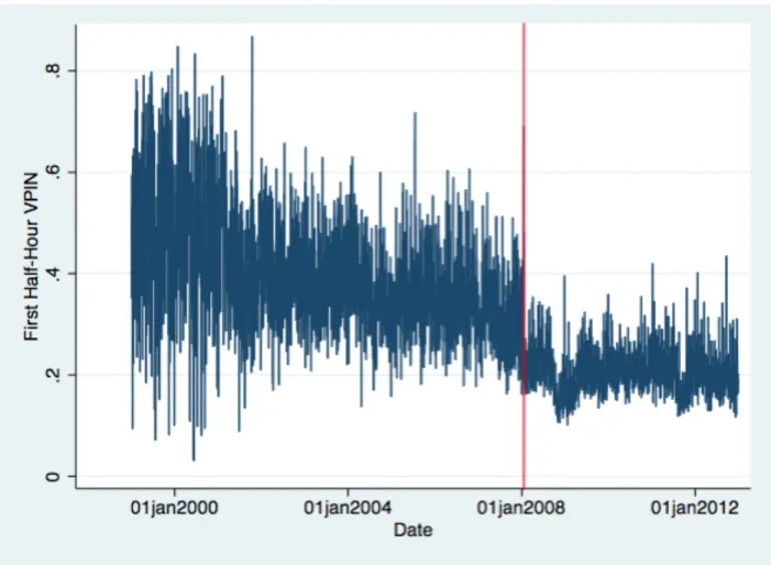
Another concern regarding the robustness of the results is that the distribution of VPIN
appears to change around the beginning of the year 2008 (Figure 7, appendix). Particularly, the
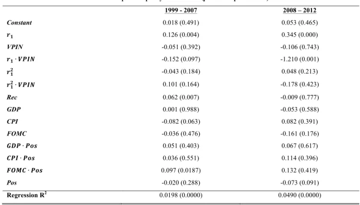
mean VPIN of the sample before this point is 0.397, while the mean VPIN after is 0.207. The sample is split at this point and the regression is estimated again for each subsample. In the first
subsample, the only major change is that the crossed return/VPIN term does not have a
significant coefficient. In the second subsample, the significance of each coefficient estimate is
approximately the same as the entire sample (Table 4, appendix). The explanatory power of the
second subsample is much greater, and the actual coefficient estimates are quite different. This is
likely due to the Great Recession, which takes up a large portion of this period.
Gao, et al also develop a trading strategy in their paper to take advantage of their
predictions (2014). The strategy is to buy or sell short during the last half hour based on the
return of the first half hour (long if the first hour returned positive, and short if the first
half-hour returned negative). For an investor using this trading strategy, a prediction of the exact
magnitude of the last half hour return may be of less interest than a prediction of a probability
that the sign of the last half-hour will match the sign of the first (and thus providing a positive
return to their investment during the last half-hour).
The probability of a successful prediction of the sign of the last half-hour return, given
the sign of the first half-hour return can be estimated by probit regression. This model could
!!!!!!!!!!!!!!!!!!!!!!!!!!!!!!!!!!!!!!!!!!!!!!!!!!!!!!!!
include each of the factors mediating the prediction of the last half-hour return. Such an
unrestricted model would be:
Pr !"! =!!+!!!!,!+!!!"#$!,!+!!!!,!∙!"#$!,!+!! !!,! !+!! !!,! !∙!"#$!,!+!!!"#!
+!!!"#$!+!!!"#!,!+!!
where !"! is a binary variable that equals 1 if the sign of the first half hour return is the same as
the sign of the last half hour return, and equals 0 otherwise. This model has a significant
explanatory power, as the !! statistic has a significant p-value (p = 0.0433). In the estimation of
this model, the crossed return/VPIN term has negative marginal effects, and is not statistically significant (Table 3, appendix). This is further evidence against the theoretical explanation by
Gao, et al. that the intraday momentum is due to the market timing of informed traders.
Another possible violation to Gauss-Markov assumptions in the above regressions that
must be considered is the potential multicollinearity among the regressors. Analysis of
correlations among regressors indicates that there are none with strong correlations besides the
correlation between Pos and the first half-hour return (Table 2, appendix). Removal of this factor does not drastically change the coefficient estimates, so it is deemed not a concern. Furthermore,
analysis of variance inflation factors (VIF) indicate that there is not much risk for collinearity
among regressors as the greatest VIF was 6.22, with a mean VIF of 3.05.
Finally, the OLS regressions only consider a linear functional form. Since Gao, et al.
found that the variability of the first half-hour return was significant for their prediction, we
hypothesize that a form with threshold effects might fit the data better. Such a model would
exhibit an increase in the predictive power of the first half-hour return on the last half-hour above
a given threshold in the first half-hour probability of informed trading or the magnitude of the
thresholds above which the predictive power is any stronger. Since no obvious threshold is
observed, the model was estimated by quintile of VPIN. First, only observations in the second quintile or above were considered, then the third or above, etc. In this methodology, the quintiles
are each used as the thresholds. The estimation coefficients differ in each regression, but in none
of these five regressions were any of the VPIN term coefficients significant and positive. The
VPIN and returns crossed term (!!) is positive but not significant in the regression including only
the observations in or above the second quartile of VPIN (Table 5, appendix). Given these results, thresholds are not considered further.
8. Conclusions
Gao, et al. hypothesize that the first half-hour return predicts the last half-hour return due
to the timing of the market entry of informed traders. Specifically, these traders enter in the first
and last half-hours. If this hypothesis is true, then increasing the probability of informed trading
during the first half-hour should increase the predictive power of the first half-hour return on the
last half-hour return. The estimation of empirical models explaining the last half-hour return with
the first half-hour return, the first half-hour probability of informed trading (as measured by
VPIN), and other factors do not indicate that a greater degree of first half-hour informed trading significantly increases the predictive power of the first half-hour return on the last half-hour
return.
In the OLS estimation, the effect of VPIN on the predictive power of the first half-hour return is in fact significant and negative. This directly violates the theoretical explanation given
return is positive in both models, but much greater in the current study model. The negative
coefficient on the crossed return and VPIN term may “cancel out” the effect of the increase in the return coefficient. This would mean that the VPIN actually does not have a significant impact on
the relationship between the first and last half-hour returns.
The inclusion of the ARCH and GARCH lags to control for autocorrelation change the
value of the !! coefficient on the crossed return/VPIN term from negative to positive. However,
this coefficient is not statistically significant (in contrast to the expected positive, significant
coefficient). In addition, the return/VPIN interaction coefficient is negative and statistically insignificant in a model only predicting the sign of the last half-hour return.
According to the theoretical explanation given by Gao, et al. (2014), the predictive power
of the first half-hour return on the last half-hour return should be positively correlated with the
first half-hour VPIN. However, in the OLS model to predict the last half-hour return, the GARCH(3,3) model to correct for autocorrelation, and the probability model estimating the
predictive power of the sign of the first half-hour return on just the sign of the last half-hour
return, this is not the case. Therefore, it can be concluded that probability of informed trading
does not positively impact the predictive power of the first half-hour return on the last half-hour
return, and the explanation provided by Gao, et al. (2014) is not supported.
There are a few limitations to this study that should be noted. The VPIN metric is an extension of the PIN model created by Easley, et al. in 1996. Duarte and Young (2009) have
found that the PIN measure is biased by positive order flow shocks to the number of both buyers and sellers, and have created an adjusted PIN measure that corrects these effects. It decomposes
component is correlated with asset returns, but Duarte and Young observe no correlation
between the corrected PIN component and asset returns (2009). Duarte and Young do not test the
VPIN model, only the PIN, so it is unknown if the VPIN model is biased by the same effect. It is
reasonable to be concerned that VPIN is a biased estimate of the probability of informed trading.
In the future, replication of this study using the Duarte and Young adjusted PIN measure
in the place of VPIN may help to provide a more complete evaluation of the explanation given by Gao, et al. for the predictive power of the first half-hour return on the last half-hour return. In
addition, the Lee-Ready algorithm could be used to assign buy and sell designation to trades
(Lee, Ready, 1991). Finally, future evaluation of the other untested explanation (see footnote,
Section 2) is necessary to find a complete explanation for the intraday momentum observed by
9. References
Admati, A. R., Pfleiderer, P., 1988. A Theory of Intraday Patterns: Volume and Price
Variability. Review of Financial Studies 1, 3-40.
Asness, C. S., Moskowitz, T. J., Pedersen, L. H., 2013. Value and Momentum Everywhere.
Journal of Finance 68, 929-985.
Bodie, Z., Kane, A., Marcus, A. J., 2011. Investments. New York, NY: McGraw-Hill Irwin.
Bollerslev, T., 1987. A Conditionally Heteroskedastic Time Series Model for Speculative
Prices and Rates of Return. The Review of Economics and Statistics, 69, 542-547.
Crombez, J., 2001. Momentum, Rational Agents and Efficient Markets. The Journal of
Psychology and Financial Markets 2, 190-200.
Duarte, J., Young, L., 2009. Why is PIN priced? Journal of Financial Economics 91, 119- 138.
Easley, D., Kiefer, N. M., O’Hara, M., Paperman, J. B., 1996. Liquidity, Information, and
Infrequently Traded Stocks. Journal of Finance 51, 1405-1436.
Gao, L., Han, Y., Li S. Z., Zhao, G., 2014. Intraday Momentum: The First Half-Hour Return
Predicts the Last Half-Hour Return. Working Paper, Washington University in St. Louis.
Hora, M., 2006. Tactical Liquidity Trading and Intraday Volume. Working Paper, Credit Suisse
Group.
Jain, P. C., Joh, G.-H., 1988. The Dependence between Hourly Prices and Trading Volume.
Journal of Financial and Quantitative Analysis 23, 269-283.
Jegadeesh, N., Titman, S., 1993. Returns to Buying Winners and Selling Losers: Implications for
Karyampas, D., Paiardini, P., 2011. Probability of Informed Trading and Volatility for an ETF.
Working Paper, Credit Suisse Group.
Kahneman, D., Tversky, A., 1972. Subjective Probability: A Judgment of Representativeness.
Cognitive Psychology 3, 430-454.
Kahneman, D., Tversky, A., 1973. On the Psychology of Prediction. Psychology Review 80,
237-251.
Lee, C. M. C., Ready, M. J., 1991. Inferring Trade Direction from Intraday Data. Journal of
Finance 46, 733-746.
MacKinlay, C., 1997, Event Studies in Economics and Finance. Journal of Economic
Literature 35, 13-39.
Schulmeister, S., 2009. Profitability of Technical Stock Trading: Has it Moved from Daily to
Intraday Data? Review of Financial Economics 18, 190-201.
Tannous, G., Wang, J., Wilson, C., 2013. The Intraday Pattern of Information Asymmetry,
Spread, and Depth: Evidence from the NYSE. International Review of Finance 13,
10. Appendix
Table 1. Summary Statistics
Sample Size Mean Standard Deviation Minimum Maximum
!! (%) 3497 0.011 0.740 -8.015 4.430
!!" (%) 3495 -0.003 0.395 -4.134 3.131
VPIN 3520 0.329 0.136 0.031 0.868
PS 3521 0.525 0.499 0.000 1.000
!!! 3497 0.547 1.745 0.000 64.233
Notes: In this table, summary statistics are presented for the continuous variables utilized in this study. The variables and their sources are defined in Table 6.
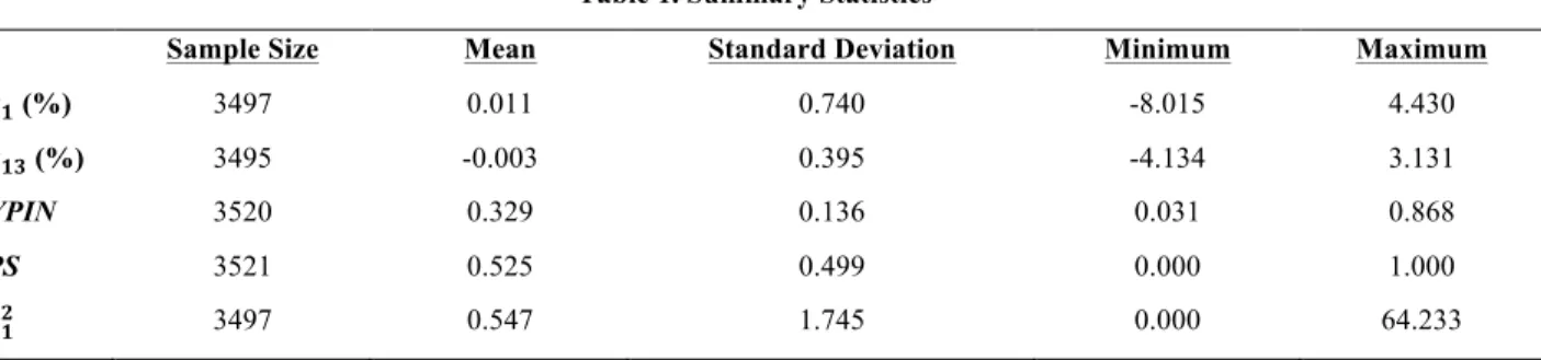
Figure 1. First and Last Half-Hour Returns, over time
!
Notes: This graph shows the return of the SPY during the first half hour of each trading day (blue), and the last half-hour of each trading day (red). The two processes appear to mirror each other, besides the outlier in the first half-hour return (due to the terrorist attacks of 9/11/2001).
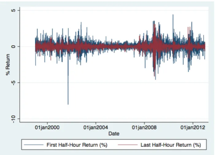
Figure 2. First Half-Hour Return, Squared, over time
!
Notes: This graph shows the squared return of SPY during the first half-hour throughout the sample period. As above, there is a spike on 9/17/2001, due to the negative trading on this day,
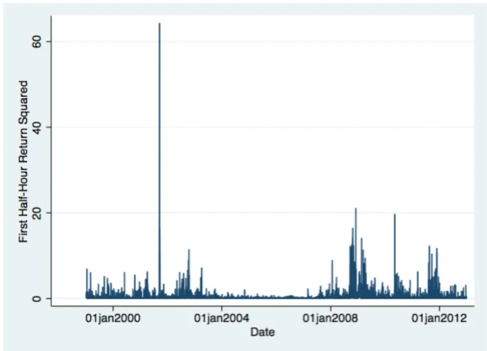
Figure 3. First Half-Hour Return Distribution
! !
Notes: The distribution of the first half-hour return is approximately Gaussian, with the mean of approximately 0%.
Figure 4. Last Half-Hour Return Distribution
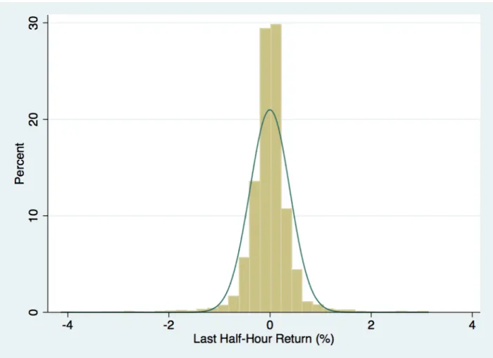
! !
Notes: The distribution of the last half-hour return of the SPY is approximately Gaussian, with a
Figure 5. First Half-Hour Return, Squared, Distribution
! !
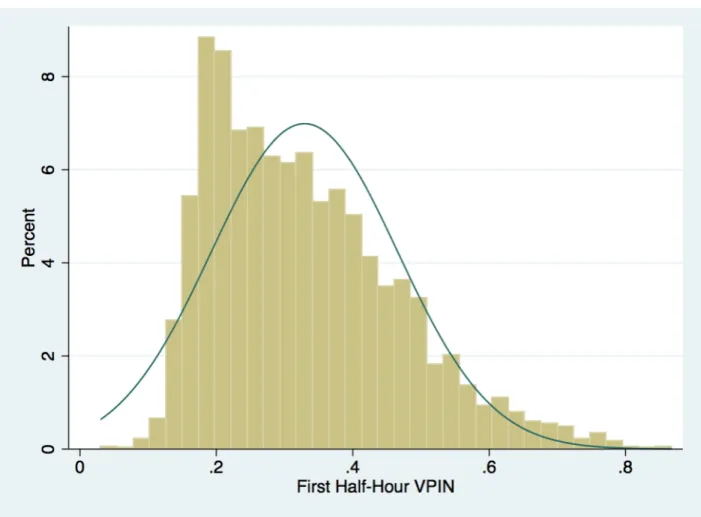
Figure 6. First Half-Hour VPIN Distribution
! !
Notes: The distribution of the first half-hour VPIN is approximately normally distributed, but with a slight skew to the right.
! ! ! !
Table 2. Correlations
!! !!" !"#$ !!! !"# !"# !"# !"#$ !"# !! 1.000 - - - - !!" 0.139 1.000 - - - -
!"#$ 0.035 -0.014 1.000 - - - -
!!! -0.166 0.016 -0.084 1.000 - - - - -
!"# -0.071 0.022 -0.179 0.188 1.000 - - - -
!"#! 0.022 0.012 0.009 -0.010 -0.004 1.000 - - - !"#! -0.012 0.002 -0.003 -0.005 -0.002 -0.051 1.000 - -
!"#$! 0.012 -0.010 0.004 -0.020 -0.002 0.035 0.028 1.000 -
!"#! 0.679 0.066 0.025 -0.028 -0.057 0.010 -0.002 -0.010 1.000
!
Notes: This table lists the correlations between each of the regressors in this study. The variables are all defined in Table 6. There are no regressors whose correlations indicate a degree of
collinearity that is troublesome for the estimation in this study.
!
Table 3. Regression Results (p-values in parenthesis)
Gao, et al. (2014) Gao Extended OLS with VPIN GARCH(3,3) Pr(PS)
Constant -0.004 (0.597) 0.016 (0.198) 0.016 (0.459) 0.026 (0.047) 0.534
!! 0.074 (0.000) 0.101 (0.000) 0.152 (0.000) 0.054 (0.002) 0.047 (0.089)
VPIN - - 0.009 (0.857) -0.059 (0.063) -0.107 (0.117)
!!∙!"#$ - - -0.189 (0.002) 0.034 (0.496) -0.093 (0.249)
!!! - 0.009 (0.022) 0.020 (0.038) 0.014 (0.150) 0.023 (0.094) !!!∙!"#$ - - -0.036 (0.192) -0.044 (0.060) -0.005 (0.907)
Rec - 0.025 (0.172) 0.021 (0.251) 0.013 (0.331) -0.010 (0.671)
GDP - -0.014 (0.753) -0.015 (0.751) -0.002 (0.947) 0.022 (0.584)
CPI - -0.017 (0.706) -0.019 (0.678) -0.022 (0.361) 0.007 (0.858)
FOMC - -0.079 (0.135) -0.079 (0.133) 0.008 (0.794) 0.040 (0.395) !"#∙!"# - 0.061 (0.33) 0.060 (0.332) -0.013 (0.719) -
!"#∙!"# - 0.053 (0.391) 0.057 (0.356) 0.023 (0.501) -
!"#$∙!"# - 0.110 (0.145) 0.111 (0.141) 0.027 (0.550) -
Pos - -0.057 (0.003) -0.049 (0.011) -0.028 (0.016) -0.009 (0.710)
ARCH CONS. - - - 0.003 (0.000) -
ARCH L1 - - - 0.148 (0.000) -
ARCH L2 - - - 0.073 (0.000) -
ARCH L3 - - - 0.121 (0.000) -
GARCH L1 - - - 0.342 (0.000) -
GARCH L2 - - - -0.424 (0.000) -
GARCH L3 - - - 0.727 (0.000) -
Regression R2 0.0193 (0.0000) 0.0247 (0.0000) 0.0278 (0.0000) (0.0000) 0.0039 (0.0424)
Notes: This table lists regression results from the empirical estimation. The first column is the model estimated by Gao, et al. (2014). The next is the model containing the untested control factors mentioned by Gao, et al. The third column is the unrestricted OLS model that includes
VPIN terms. The fourth is the GARCH(3, 3) model, and the last is the model in which just the sign of the last half hour return is predicted. The p-values for the significance of the t-statistics associated with each coefficient are in parentheses. The ARCH χ2p-value is reported in place of R2, and the Marginal Effects (means and sample sizes in Table 1) and Pseudo R2 are reported for
Figure 7. First Half-Hour VPIN over Time
! !
Notes: This figure gives the distribution of VPIN over time. There is a clear structural break at the beginning of 2008 (denoted by the red line), after which the mean value of VPIN is clearly different.
Table 4. Split Sample by VPIN Trend (p-value in parenthesis)
1999 - 2007 2008 – 2012
Constant 0.018 (0.491) 0.053 (0.465)
!! 0.126 (0.004) 0.345 (0.000)
VPIN -0.051 (0.392) -0.106 (0.743)
!!∙!"#$ -0.152 (0.097) -1.210 (0.001)
!!! -0.043 (0.184) 0.048 (0.213)
!!!∙!"#$ 0.101 (0.164) -0.178 (0.423) Rec 0.062 (0.007) -0.009 (0.777)
GDP 0.001 (0.988) -0.053 (0.588)
CPI -0.082 (0.063) 0.082 (0.391)
FOMC -0.036 (0.476) -0.161 (0.176)
!"#∙!"# 0.051 (0.403) 0.067 (0.617)
!"#∙!"# 0.036 (0.551) 0.114 (0.396)
!"#$∙!"# 0.097 (0.0187) 0.132 (0.419)
Pos -0.020 (0.288) -0.073 (0.091)
Regression R2 0.0198 (0.0000) 0.0490 (0.0000)
Notes: This table contains the regression results from the split-sample regression. The sample is split at the beginning of 2008, when there is a structural break in the distribution of VPIN. The regression before the split is in the left column, and after the split on the right. The p-values for the significance of the t-statistics associated with each coefficient are in parentheses.
Table 5. Regression by VPIN Quintile (p-value in parenthesis)
VPIN≥ 0.2039811 VPIN≥ 0.2691757 VPIN ≥ 0.345115 VPIN≥ 0.4426617
Constant -0.003 (0.894) 0.045 (0.146) 0.029 (0.554) -0.034 (0.721)
!! 0.047 (0.140) 0.125 (0.008) 0.060 (0.383) 0.277 (0.031)
VPIN 0.030 (0.198) -0.042 (0.194) -0.055 (0.177) -0.015 (0.863)
!!∙!"#$ 0.004 (0.940) -0.098 (0.144) -0.057 (0.566) 0.055 (0.747) !!! 0.019 (0.792) -0.151 (0.127) -0.019 (0.888) -0.398 (0.082)
!!!∙!"#$ -0.061 (0.26) 0.102 (0.168) 0.127 (0.165) 0.065 (0.686)
Rec 0.024 (0.196) 0.039 (0.079) 0.049 (0.093) 0.061 (0.158)
GDP -0.040 (0.344) -0.037 (0.448) -0.023 (0.720) 0.008 (0.938)
CPI -0.044 (0.279) -0.089 (0.045) -0.144 (0.017) -0.258 (0.015)
FOMC -0.014 (0.774) -0.045 (0.387) -0.051 (0.433) -0.149 (0.139)
!"#∙!"# 0.067 (0.243) 0.083 (0.192) 0.097 (0.242) 0.171 (0.186) !"#∙!"# 0.015 (0.791) 0.016 (0.798) 0.066 (0.419) 0.109 (0.440)
!"#$∙!"# 0.072 (0.303) 0.103 (0.173) 0.169 (0.081) 0.342 (0.017)
Pos -0.019 (0.297) -0.020 (0.304) -0.038 (0.145) -0.039 (0.306)
R2 0.0113 (0.0030) 0.0197 (0.0001) 0.0208 (0.0068) 0.0524 (0.0004)
Notes: This table gives the regression results of the tests for threshold effects. Each regression uses the given value of VPIN at the top of the column as the threshold, as no threshold is immediately apparent. The p-values for the significance of the t-statistics associated with each coefficient are in parentheses.
Table 6. Variable Definitions and Sources
Short Variable Name Full Variable Name Definition Source
!! First Half-Hour Return The percent return of the SPY during the first half-hour of the trading day
Wharton Research Data Services (WRDS) NYSE Trade and Quote (TAQ) Database
!!" Last Half-Hour Return The percent return of the SPY during the last (13th) half-hour of the trading day
WRDS NYSE TAQ Database
VPIN First half-hour Volume-Synchronized Probability of Informed Trading
The VPIN of the SPY during the
first half-hour of the trading day WRDS NYSE TAQ Database
!!! First half-hour return, squared The percent return of the SPY during the first half-hour of the trading day, squared
WRDS NYSE TAQ Database
Rec Recession Dummy variable that equals 1 if in a recession, 0 otherwise
National Bureau of Economic Research (NBER)
GDP GDP Release Date Dummy variable that equals 1 if there is a GDP release on that day, 0 otherwise
US Bureau of Economic Analysis (US BEA)
CPI CPI Release Date Dummy variable that equals 1 if there is a CPI release on that day, 0 otherwise
US Bureau of Labor Statistics (US BLS)
FOMC FOMC Minutes Release Date Dummy variable that equals 1 if there is a FOMC meeting minutes release on that day, 0 otherwise
US Federal Reserve
Pos Positive First Half-Hour Return Dummy variable that equals 1 if the first half-hour return of the SPY is positive on that day, 0 otherwise
WRDS NYSE TAQ Database
PS Predicted Successfully Dummy variable that equals 1 if the sign of the last half-hour return is predicted successfully from the sign of the first half-hour return on that day, 0 otherwise.
WRDS NYSE TAQ Database