2017_Carter.pdf

(1)

Phonological Activeness Bias Effects in Language Acquisition and

Language Structuring

By William Carter

Honors Thesis Linguistics

University of North Carolina – Chapel Hill

2017

Approved:

(2)

Abstract

The task of language acquisition constitutes an inductive problem in which learners must generalize numerous productive linguistic patterns with only a small subset of all potential inputs as the learning data (Chomsky, 1980; Pinker, 1979). Faced with this “poverty of the stimulus” (Chomsky, 1980), the need for inductive generalization is apparent, and previous work shows that a set of biases that reduce the set of viable generalizations to consider and facilitate choosing certain generalizations over others are required to extrapolate patterns beyond the initial learning data (Mitchell, 1990; Wilson, 2006). Therefore, the identification of domain-general and

language-specific inductive biases pertaining to language acquisition is fundamental in constructing an accurate model of human language learning and has been the focus of many studies (Becker et al., 2011; Moreton, 2008; Pater & Moreton, 2012; Wilson, 2006 among others).

The current project proposes the existence of one such inductive bias in the phonological domain towards acquiring pattern generalizations which make use of features that are already more phonologically active in a learner’s grammar(s). Here, phonological activeness is defined as the relative degree to which a certain feature (e.g. [voice]) is referenced in the denotations of natural classes in the phonological component of a learner’s grammar (acquired phonological patterns and phonotactic distributions). The proposed bias, which favors reimplementing features proportional to their activeness, constitutes an example of a preferential attachment process (also called a cumulative advantage or Yule process) (Price, 1976).

Evidence for this phonological activeness bias is found by observing its predicted effects in language acquisition via an artificial language learning task in which 100 English

monolinguals learned sound alternations triggered either by an active feature of English, [+/- front], or an inactive feature, [+/- high]. Trends suggest that English speakers were able to better learn the pattern triggered by [+/- front], supporting a bias towards acquiring patterns involving active features. This indicates that learners aren’t simply biased towards acquiring/implementing patterns motivated by L1 rules in another language as suggested in Pater & Tessier (2006), but rather that they are more primed to “notice” and then acquire novel patterns implementing features used frequently in their L1 phonology (English in this case). In addition, intra-language distributions of feature frequencies for a sample of phonological rules/phonotactic distributions closely fit the predicted frequency distributions generated by a well-known preferential

(3)

Acknowledgments

Although this project bears my name, there are so many wonderful people without whom it would have never been possible, and I would like to give them their due credit here. Firstly, I would like to thank my advisor, Dr. Elliott Moreton, for his invaluable expertise and guidance which were central in molding my raw ideas into cohesive and testable hypotheses, and also his general enthusiasm for research which made this project a joyful undertaking. Out of our collaboration, I have been endowed with a clearer understanding of the path I hope to pursue in the coming years, and a role model to guide me along the way. Secondly, I would like to thank Drs. Katya Pertsova and Jennifer Smith, members of my committee, for their incredibly

insightful comments and critique.

In addition, I would also like to thank Chris Wiesen of the UNC Odum Institute for his huge help with statistic interpretation and analysis of experiment results. I am grateful to members of the UNC P-Side group (Jennifer Boehm, Haley Boone, Emily Moeng, Yuka

Muratani, Amy Reynolds, and Mika Wang) and the whole Linguistics department for creating a stimulating environment for research and discussion.

Crucially, this project would never have been feasible were it not for the generous support of the Tom and Elizabeth Long Excellence Fund for Honors administered by Honors Carolina. Thank you not just for providing me this opportunity, but for your engagement in inspiring and promoting a new generation of researchers and scholars.

(4)

1. Introduction

In the aim of better understanding the learning mechanism(s) which underlie the processes of language acquisition, a body of research has emerged that is concerned with

identifying a set of domain-general and/or language-specific inductive biases that push language learners to favor the formulation of certain generalizations from their language exposure (Becker et al, 2011; Hayes & White, 2013; Pater & Moreton, 2012; Pater & Tessier, 2006; Prickett, 2014; Moreton, 2008; Seinhorst, 2016; Wilson, 2006). Given the relatively limited amount of language input from which language learners must and do consistently identify and internalize numerous patterns, such biases must exist which restrict consideration to a small set of viable

generalizations (Chomsky, 1980; Mitchell, 1980). The need for these biases in a robust system of linguistic induction is covered in further detail in §2.1. Subsequently, examples of some

inductive biases relevant in phonological learning will be briefly reviewed in §2.2, and evidence that inductive biases may play a sizeable role in phonological typology is considered in §2.3.

The current project aims to test the existence of one such inductive bias which favors the acquisition of patterns utilizing phonologically active features. Here, I assume the definition of phonological activeness given in (1):

(1) Phonological Activeness: For a particular feature, its phonological activeness is directly proportional to the absolute count frequency (either type or token) with which said feature is used to define the natural classes of segments involved in phonological rules and phonotactic distributions in a speaker’s grammar1_.

Therefore, features that appear more frequently are considered that much more phonologically active in a speaker’s grammar.

Since the proposed bias favors the reimplementation of already phonologically active features when acquiring a new rule or distribution, this bias exemplifies preferential attachment, or a “rich-get-richer” effect, through which a few features should become especially active in a single language while most features remain relatively inactive. A background on preferential attachment effects and some examples language are covered in §2.4. In §2.4.1, I introduce a specific model of preferential attachment, the Indian Buffet Process (IBP) (Griffiths & Ghahramani, 2005, 2011), which can generate a family of feature frequency distributions associated with preferential attachment processes.

Given that the step-by-step order in which learners identify and acquire patterns is entirely opaque and almost certainly idiosyncratic for every learner, directly observing the proposed phonological activeness bias in action in natural language is improbable to say the least. Therefore, this project considers two means of testing for the presence of the bias by looking for its predicted effects:

1_{Mielke (2008) defines phonologically active classes as groups of sounds that trigger or undergo a common}

(6)

(2) Tests for the Presence of a Phonological Activeness Bias

1. Do natural languages exhibit a feature activeness distribution in their

phonological components (rules and distributions) consistent with a preferential attachment process?

2. In an artificial learning task, will language learners learn a sound pattern triggered by a feature that is active in their native grammar more easily than a pattern triggered by an inactive feature?

For both of the questions posed in (2), the simple answer should be “yes” if the proposed bias towards phonologically active features exists and exhibits preferential attachment properties. Towards answering the first question, the first component of this project is a corpus study using PBase (Mielke, 2008), a collection of phonological rules and phonotactic distributions for numerous languages. By retrieving the features used to denote the natural classes involved in these rules and distributions, a feature activeness distribution for each language is constructed and compared with the best-fitting IBP model in order to test for similarity. This study finds that natural language feature activeness distributions closely fit preferential attachment distributions. The design and results of the corpus study are covered in detail in §3.

As for the second question posed in (2), an artificial language learning study based heavily on another study appearing in Pater & Tessier (2006) was conducted in which 100 native English-speaking participants learned a pattern of word-initial “t” epenthesis. The participants were divided into two groups; the first group learned “t” epenthesis triggered by word-initial front vowels while the second group learned a pattern of “t” epenthesis triggered by word-initial high vowels. In English, [+/- front] is more phonologically active than [+/- high], and so it is predicted that the pattern triggered by vowel frontness should be learned more successfully, and findings corroborate this prediction, for the frontness group was more accurate in applying “t” epenthesis after the learning task. The design and results of the artificial learning task are

covered in detail in §4 (also, see §2.5. for evidence regarding the suitability of artificial language tasks to studying natural language).

In §5, I have briefly summarized the findings of the two component studies of this project and discuss the overarching implications and potential avenues of further study on this topic. The complete stimuli set for the artificial learning task (in IPA) as well as feature frequency

distributions are included in the appendix, §6.

2. Background

2.1. The Need for Inductive Biases

The task of language acquisition is a massive undertaking on account of the numerous patterns a learner must recognize and internalize from a relatively limited subset of all possible inputs of the language system being acquired. In other words, language acquisition cannot simply be a process of memorizing all possible sentences or every word form, because (1)

(7)

finite, incredibly small collection of potential forms. In order to overcome this “poverty of the stimulus” (Chomsky, 1980), a robust system of induction which facilitates the identification of patterns in the input stream and the productive application of these patterns to novel inputs is necessary (Pater & Moreton, 2012; Pinker, 1979, 2004). Not only must such a system be innate in order to account for the shared ability of all unimpaired language learners to successfully complete the task, but the need for a language-specific cognitive module, often referred to as Universal Grammar (Chomsky, 1980; Cook & Newson, 2014), is also widely accepted since humans are not as consistently successful in pattern learning across all cognitive domains.

To somewhat complicate matters, more recent work observes the existence of surplus patterns in the input which learners seem to overlook or disregard, leading to the positing of a “surfeit of the stimulus”, the existence of too many potentially learnable patterns (Becker et al., 2011; Hayes & White, 2013; Prickett, 2014). Therefore, a viable system of induction must be capable of simultaneously parsing language data for a set of linguistically valid patterns and filtering the set so as to dismiss unintended purely coincidental patterns. By utilizing a series of biases or constraints on viable linguistic patterns, such a feat is possible.

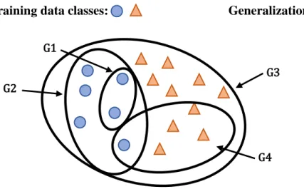
The need for such a set of biases to feasibly limit and identify viable generalizations becomes apparent when one considers the futility of an unbiased system as considered in Mitchell (1980). Firstly, one can see that a remarkably large number of generalizations can possibly be made from a finite training data set as illustrated in Figure 2.1:

Fig. 2.1. For any learning data set, a large number of generalizations are possible for an

unbiased learner

training data classes: , Generalization:

In Figure 2.1, we see a scenario in which an unbiased learner is given a training dataset of circles and triangles. Four example generalizations are illustrated. However, every possible subset (the power set) of the entire training set is a viable generalization for the unbiased learner. For an unbiased learner, the only goal of learning is to be able to correctly capture the training data, and so no concern for the external implications of a generalization for classifying novel inputs is given. That is, since G4 is just as valid in capturing a subset of the learning data as G2, the learner has no reason to disregard such a generalization. However, this should seem

especially egregious, since weintuit that the data should be grouped together by their shape G4

G3 G1

(8)

characteristics. The result that an unbiased learner cannot differentiate or rule out possible generalizations from a training data set clearly indicates the need for inductive biases to guide learning, Mitchell (1980) concludes. The idea that generalizations should encompass a set of instances with common features would be one example of a bias. This would effectively eliminate generalizations G3 and G4, leaving G1 and G2, and the preference for G2 could be explained with a bias towards maximum generalization.

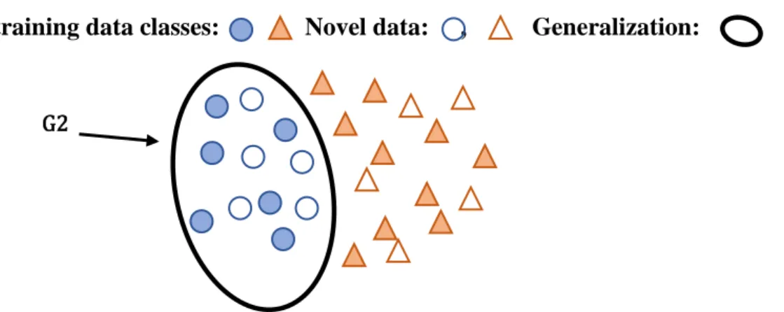
Fig 2.2. By implementing biases, the learner can decide on a likely generalization and

make accurate predictions when classifying novel instances

training data classes: , Novel data: , Generalization:

Given these suggested biases, the learner is now capable of choosing a best generalization from all of the theoretical possibilities, G2. As a result, the learner is able to make classification predictions beyond the training data as demonstrated in Figure 2.2, correctly classifying novel instances of circles as members of the same class generalization as the training circles.

In summary, the need for an innate inductive system of language acquisition is clear given the widely-accepted existence of a “poverty of the stimulus”, the fact that only a small set of possible forms are encountered in language exposure (Chomsky, 1980). With the added existence of a “surfeit of the stimulus”, the presence of coincidental patterns/generalizations, learners must implement a series of inductive biases in order to rule out linguistically unviable patterns given the failings of an unbiased learning process. (Becker et al., 2011; Hayes & White, 2013; Mitchell, 1980).

2.2. Inductive Biases in Phonological Learning

Since biases are so crucial for any robust system of generalization, linguists stand to make significant progress towards an accurate model of language acquisition by identifying the domain-general and language-specific biases relevant to acquisition. In light of this, a sizeable body of research has emerged with exactly this aim (Becker et al., 2011; Hayes & White, 2013; Moreton & Pater, 2012; Pater & Tessier, 2006; Pater & Moreton, 2012; Prickett, 2014; Saffran, 2003; Seinhorst, 2016; Wilson, 2006 to name a few). In this section, some well-attested inductive biases are highlighted and briefly discussed.

(9)

Pattern Complexity

To the scholar faithfully applying Ockham’s Razor, structural parsimony of a model is a merit and the comparative simplicity of two otherwise identically data-consistent models for some phenomenon is a strong basis for favoring one (the simpler) over the other. The goal here is to minimize the necessary assumptions for the model to hold true, thereby maximizing its

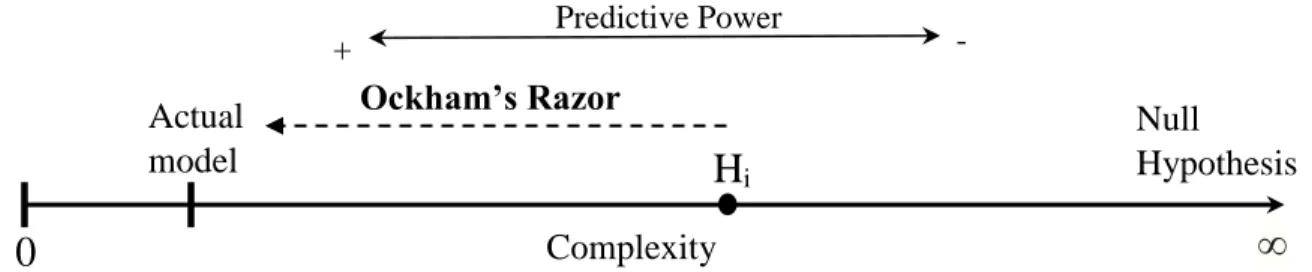
falsifiability and predictive power. One can see that the maximization of simplicity is a fruitful guide in hypothesis construction on account of the fact that it tends towards a definite endpoint, finding the actual necessary and set of factors that explain an effect. In stark contrast, the null hypothesis claims that no patterns exist and therefore can never make any predictions for novel data from the prior experience. Hypothesis complexity and the need for Ockham’s razor in guiding the pursuit of the best model from infinite possibilities is illustrated in Figure 2.3:

Fig. 2.3. On a hypothesis complexity continuum, aiming towards simplicity has the result

of maximizing predictive power and has a definite limit.

In Figure 2.3, the learner begins with the initial hypothesis, Hi, which accurately captures

all current data. The learner has three options: (1) keep the model until new evidence invalidates it, (2) throw out any model and accept the Null Hypothesis, and (3) try to simplify the model. The third option is most preferable since it has the potential to eliminate unnecessary

assumptions, maximize predictive power, and approach the actual model.

Methodological proselytization aside, such a bias towards simplicity is not restricted to high level reasoning and plays a strong role in guiding machine learners towards the production of highly-predictive generalizations from a learning data set as seen in a proof by Blumer et al. (1987) who demonstrate that the existence of an Ockham’s Razor learning algorithm for any learning task facilitates the formation of an accurate generalization hypothesis in polynomial (efficient) time. Therefore, the existence of such an algorithm with a bias towards simplicity could be one possible explanation for the efficiency and across-the-board success with which humans acquire a (first) language.

Experimental linguistic data supports the existence of a complexity bias in language acquisition. For example, Saffran & Thiessen (2003) tested the ability of infants to recognize and internalize artificial language patterns of varying complexity across two experiments (the second and third experiments in the paper). In the first experiment (experiment two), infants were

divided into two groups. The first group was exposed to artificial language training data in which only /p, t, k/ could appear word-initially, and the second group learned that only /b, d, g/ could

H

i

0 ∞

Actual model

Predictive Power

+ -

Complexity

(10)

appear word-initially. In both conditions, the pattern could be abstracted to “classes” of segments linked by their value for [+/-voice]. That is, only one distinction was necessary to describe the target pattern. Both patterns were learned equally successfully by infants with no regard to whether the word-initial class consisted of [+voice] or [-voice] stops. In a second experiment (experiment three), Saffran & Thiessen tested the ability of infants to learn a pattern where viable word-initial segments were /p, d, k/ or /b, t, g/. These “inconsistent” patterns as they call them were not learned as consistently or as successfully by infants as the [+/- voice] patterns

considered in the previous experiment. The important observation to make is that more than one distinction is necessary to describe the class of viable word-initial segments.

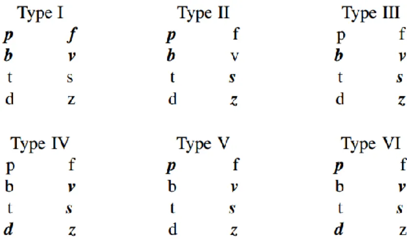
These results are strongly indicative of a complexity bias in the language acquisition toolset available to infants, where complexity is tied to the number of distinctions necessary to capture a pattern. Such a conceptualization of complexity has been proposed and demonstrated by Shepard et al. (1961) who found that the number of features/distinctions needed to describe generalizations influenced learning success in the visual domain, and that patterns with fewer distinctions were more learnable. Linguistic-domain examples of Shepard et al.’s pattern complexity classes are given in Figure 2.4 (taken from Pater & Moreton, 2012).

Fig. 2.4. The more distinctions needed to capture a class of segments in a pattern, the

more complex the pattern. For example, Type I requires one feature to capture bolded segments, [+labial]. In comparison, Type II requires two features and two classes, [+labial, -cont] OR [-labial, +cont]. Types III – VI require three features. Taken from Pater & Moreton (2012) (see source, pp. 26-28 for more in-depth discussion of pattern types and complexity).

(11)

Phonological Naturalness

A second proposed inductive bias is pattern “naturalness” which refers to the typological attestedness or presence of phonetic motivation for a certain pattern (Becker et al., 2008; Hayes & White, 2013; Prickett, 2014). That is, natural patterns are those which are attested in at least one known natural language and/or have phonetic motivations. In a study of Turkish root-final laryngeal alternations in nouns, Becker et al. (2008) find that lexical statistics indicate three factors (patterns) associated with the laryngeal alternations: final stop place of articulation (PoA), noun size, and preceding vowel quality. Of those three, native Turkish speakers showed awareness of only the PoA and noun size patterns when applying them to nonce words in a forced choice task, and showed no effects of preceding vowel quality. The existence of

patterns/generalizations in the lexical statistics that language learners seem to ignore or dismiss led Becker et al. to posit a “surfeit of the stimulus” (too many patterns), and the need for biases accounting for the acquisition of some patterns which are phonologically natural/viable, and not others.

Work by Hayes & White (2013) corroborates Becker et al.’s (2008) findings. Using the Hayes/Wilson Phonotactic Learner (Hayes & Wilson, 2008), they generated a set of 160 phonotactic constraints of varying weights from a training data set of American English. Like Becker et al., not all of the found constraints were apparently phonetically motivated and/or typologically well-represented. Taking ten examples of “natural” constraints and ten examples of “unnatural constraints”, they then tested English speakers’ grammaticality (goodness) judgments for nonce words violating each of the constraints. They found that natural constraint violations resulted in a larger decrease in goodness judgments than unnatural constraint violations

compared with control judgments for non-violating nonce words. This suggests that unnatural constraints and patterns are not acquired by native speakers of a language.

Teasing apart phonological naturalness from phonological complexity under the proposed definition does not seem like a purely straight forward task, for it is imaginable that complexity (or any other array of inductive biases) could be a determiner of naturalness. As Saffran & Thiessen (2003) point out in their discussion, the fact that infants more successfully acquire the simpler /p, t, k/ pattern over the more complex /p, d, k/ pattern might suggest that few languages (if any) should ever exhibit a /p, d, k/ class. In this way, naturalness as defined on typological grounds would be an emergent quality of complexity-biased acquisition with no direct

relationship to the language acquisition procedure itself.

A study by Prickett and Moreton (2014) tackles exactly this issue by performing a two-dimensional analysis of complexity and naturalness, breaking down phonotactic constraints into natural simple, natural complex, unnatural simple, and unnatural complex categories. Sampling representative members of each category from the 160 constraints identified by the

(12)

by comparison. Prickett point out that this seems to contradict artificial language studies finding strong effects of pattern complexity, and posit that this indicates a difference in natural and artificial language acquisition, or native and second language acquisition more broadly.

Transitional Probability

The last proposed bias to be considered in this review, transitional probability, is representative of a larger body of work investigating statistical learning and its application in language acquisition and more general learning procedures (Saffran, 2003; Bonatti et al., 2005; Moeng, 2016). As its name suggests, transitional probability denotes the probability of

transitioning to one state from a given current state. In the domain of language, Saffran (2003) proposes syllabic transitional probability as a tool for word segmentation, one of the qualities of language which infants must learn without pauses in fluent speech. In terms of syllables, words represent immutable bundles of syllables, meaning that every instance of the word “linguist” would increase the probability of the transition “lin”“guist”. By comparison, transitions across word boundaries are almost completely unpredictable (ignoring syntax/semantics), so numerous cross-word-boundary transitions will be attested, each with a very low probability given the huge number of possibilities across which the probability must be distributed. In summary, word-internal transitional probabilities are consistently higher than transitional probabilities across word-boundaries, so a statistical learner with a bias for segmenting words according to transitional probabilities would likely search for local minima in the probabilities and hypothesize a word-boundary at the location of each minimum.

2.3. Inductive (Analytic) Biases and Phonological Typology

Having considered strong evidence for the necessity of inductive biases in making successful generalizations in language acquisition (§2.1) followed by several examples of proposed biases (§2.2), it would be beneficial to discuss evidence for connections between acquisition biases and phonological typology since such a connection is necessary for the corpus study component of this project (§3) to be meaningful. As mentioned in the previous section concerning known examples of inductive biases, one can imagine cases where biases affecting the learnability of certain patterns (like a complexity bias) could affect language typology. For example, Saffran & Thiessen (2003) take the observation that infants were more successful in acquiring the simpler pattern and pair it with the observation that simple classes like /p, t, k/ ([-voice]) are more cross-linguistically common than classes like /p, d, k/, offering the explanation that differences in ease of acquisition could explain the higher representation of simple patterns in phonological typology.

(13)

consistent with natural languages. As Moreton describes, channel biases can be thought of misinterpretation of coincidental phonetic patterns, “precursors”, as phonological. Stronger precursors are more likely to result in phonologization (Blevins, 2004; Moreton, 2008; Ohala, 1994a). For example, the phonologization of vowel height agreement might occur as a result of the strong phonetic precursor of coarticulation effects (Blevins, 2004; Moreton, 2008; Ohala, 1994b). Moreton points out that, as the existence of a precursor predicts, height-height patterns are typologically widespread. However, he also notes that height-voice patterns are not nearly as typologically represented despite also possessing an equally strong phonetic precursor. This leaves only analytic biases remaining to explain typology when channel biases are insufficient to account for asymmetries like that between height-height and height-voice patterns. In Moreton & Pater (2012), the role of inductive biases in language acquisition and the emergence of

phonological typology asymmetries is summarized as a force pushing learners towards simple patterns and the rejection of complex patterns while channel biases fuel the formulation of new patterns by providing systematic phonetic precursors with the potential for phonologization (Bach & Harms, 1972).

2.4. Preferential Attachment Processes

Having shown that inductive biases can and often do play a role in generating language typology asymmetries, we can now consider the predicted typological effects of a phonological activeness bias as proposed in §1. The definition of phonological activeness assumed in this study is copied below for ease of reference:

(3) Phonological Activeness: For a particular feature, its phonological activeness is directly proportional to the absolute count frequency (either type or token) with which said feature is used to define the natural classes of segments involved in phonological rules and phonotactic distributions in a speaker’s grammar. Therefore, features that appear more frequently are considered more phonologically active in a speaker’s grammar.

e.g. In Maltese phonology, [+/- voice] is included in the definitions of 28 natural classes involved in phonological patterns documented on PBase. Therefore its phonological activeness is c*28u (“u” denotes some arbitrary unit measure of activeness; c is some positive constant2). By contrast, [+/- strident] only occurs in 6 natural classes involved in phonological patterns, so its phonological activeness is c*6u. [+/- round] is completely inactive in Maltese phonology since it occurs in no phonologically active classes.

As noted in §1, my definition of phonological activeness is inspired by that of Mielke (2008) who defines phonologically active classes as groups of sounds that trigger or undergo a

2_{Since we only care about relative phonological activeness of a language’s features and the activeness for all}

(14)

common phonological rule. My definition of phonologically active features is related to Mielke’s definition insofar as phonologically active features are the features that denote

phonologically active classes. One thing to note, is that I extend the definition of active features to also include the set of altered features (the change) in a phonological rule since this must also be learned in order for a language user to apply the rule correctly. Another important distinction is that I assume phonological activeness to be a property of features within a single grammar, and is not a measure of the frequency with which features are implemented across languages.

The goal of this project is to provide evidence for the existence of a bias favoring the acquisition of phonological patterns utilizing highly phonologically active features. Translating degree of activeness to the frequency with which a feature has already been used to capture phonologically active classes, one can see that a cyclical pattern emerges in which the likelihood of reusing a feature again increases for every time it has been used before, and this in turn increases its activeness further. This is known as a “rich-get-richer” effect.

This effect is an attested product of preferential attachment processes, also called cumulative advantage or Yule processes (Price, 1976), which assign probabilities towards selecting each feature from a list of finite possible choices in proportion to the number of times each feature has been selected prior to the current trial (Griffiths & Ghahramani, 2005, 2011). Beginning with Price (1976), preferential attachment processes have been used with success in capturing some properties of growing networks such as citation networks (like Google Scholar), the World Wide Web (Barabási et al., 2000), Wikipedia (Capocci et al., 2006), and developing semantic networks (Steyvers & Tenenbaum, 2005), all of which are considered scale-free networks exhibiting a power-law distribution. In particular, preferential attachment processes have the ability to account for the emergence of power-law (heavy-tailed) distributions in these networks resulting in the existence of a few highly-connected hubs with more numerous less-connected offshoots. For example, Figure 2.5 shows connectivity distributions from the work of Faloutsos et al. (1999) studying preferential attachment effects in the topology of the World Wide Web where each point represents a web domain plotted by degree, the number of

(15)

Fig. 2.5. A log-log plot of web domains in 1997 by their degree (number of connections)

on the x-axis and their degree-rank (place in the list of domains ranked greatest-to-least by degree) on the y-axis. The strong linear relationship that emerges is indicative of a power-law relationship between degree and degree-rank, and implies a preferential attachment effect in growth of the WWW network. Taken from Faloutsos et al. (1999).

2.4.1. Indian Buffet Process (IBP)

It is beneficial in justifying the proposal of a preferential attachment process to draw a connection between network growth as discussed above and the process of phonological pattern acquisition. Specifically, one can consider the relationship between phonological patterns (rules and distributions) and the features used to capture the relevant natural classes through the lens of an Indian buffet restaurant. This explanation is adapted to from the work of Griffiths &

Ghahramani (2005, 2011). In this scenario, the restaurant represents a language offering a fixed set of dishes from which customers can choose to form their meal. The set of dishes corresponds to the set of distinctive features present in the grammars of its speakers (Chomsky & Halle, 1968; Jakobson et al., 1952). If we imagine that every customer coming into the restaurant is a phonological pattern, then pattern acquisition becomes the drawing of links (networks) between each customer (pattern) and some number of dishes (features) which they select for their meal. In order to add preferential attachment to the mix, we simply add the ability of each customer to observe how many times each dish has been used and to infer that the most sampled dishes must be delicious, resulting in the effect that customers favor eating already popular dishes to

experimenting with untouched dishes. The process is illustrated in Figure 2.6:

Domain degree (# of connections)

D

om

ai

n deg

ree

-r

(16)

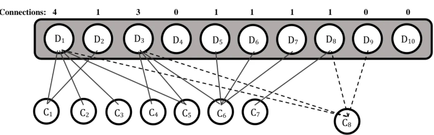
Fig. 2.6. An illustration of a pattern-feature network emerging from customers

selecting dishes at an Indian buffet restaurant. Customer 8 is now considering her

choices. Dk=dish (feature), Cn = nth customer (phonological pattern).

Connections: 4 1 3 0 1 1 1 1 0 0

As seen in Figure 2.6, customer eight comes into the restaurant and is presented with a finite selection of dishes, and can choose any combination for her meal. Some of the possible choices that customer eight can make are illustrated by the dotted lines. Under a model of preferential attachment, each pattern will be more likely to make a connection to a feature the more connections that feature already has. Therefore, one would assign customer eight choosing dish one the highest probability.

Now that we have a sense of how phonological pattern acquisition can be translated into pattern-feature network formation terms, we can pursue a more formal definition of a preferential attachment algorithm, the Indian Buffet Process (Griffiths & Ghahramani, 2005, 2011),

henceforth abbreviated as IBP. The IBP is a stochastic algorithm simulating the process illustrated above for some defined number of customers under the following assumptions:

(4) IBP Assumptions

1. The buffet is potentially infinitely long3 (i.e. There is no prior assumption as to the number of features in the data).

2. Customers come in one by one and proceed down the buffet line in the same order, taking dishes until they are satisfied.

3_{A notable difference between the proposed scenario of phonological network building and the IBP is that the IBP} was designed for use in nonparametric latent feature inference (the detection of directly unobservable features in data without prior knowledge of how many features there actually are). Therefore, it makes no prior assumptions about the number of relevant features unlike in the phonological case where the set of features is defined and finite. However, new features are only added to the mix when customers come in, and the IBP only has the possibility of finding infinitely many latent features. Therefore, every IBP has a finite end given a finite number of customers, so it will always end with a finite number of features, meaning that comparison with the phonological case is valid. This is especially true if we imagine giving an IBP every possible rule, for even if it only discovered features one at a time, it would still approximate the complete set of proposed phonological features.

D1 D2 D3 D₄ D₅ D₆ D₇ D8 D9 D10

C1 C2 C3 C4 C5 C6 C7

(17)

The IBP allows for one free parameter, α, which affects the rate at which customers incorporate new features into the mix and can be thought of as how hungry each customer is. The IBP algorithm can then be summed up as follows:

(5) IBP Algorithm

1. The first customer samples the first Poisson(α) dishes from the buffet.

(Repeat steps 2 and 3 for every remaining customer):

2. Each subsequent nth_{customer passes through the line of previously sampled dishes}

and has probability 𝑃(𝑘) =𝑚𝑘

𝑛 of choosing each dish k. (m=number of times previously sampled).

3. When the customer reaches the end of the previously sampled dishes, they sample the next Poisson(α/n) number of dishes down the buffet line.

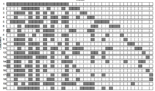
Using this algorithm, we can then apply this to the question of phonological processes and how they implement features, specifically with a rich-get-richer bias for reusing common features. The source of preferential attachment effects in the algorithm is in step 2 where the probability of choosing a previously selected dish is proportional to the number of times it has been previously selected. An example of the customer-dish matrix resulting from an IBP is provided in Figure 2.7. Shaded squares indicate that the customer selected the dish.

Fig. 2.7. The resultant customer-dish matrix of an IBP simulation. Taken from

(18)

Despite a good conceptualization of how phonological pattern acquisition could be a network building process and the existence of the IBP which provides a convincing step-by-step algorithm, the fact that we cannot observe or confidently postulate the order in which language learners acquire patterns (the order of customers) means that the predictions of the IBP are uninterpretable in their current form. What is needed is a predicted distribution of the relative probabilities/frequencies of all of the feature after completion of an IBP with n customers without regard to order.

To do this, we can implement the stick-breaking construction of the IBP (Teh et al., 2007) which has the characteristic of deriving the relative probabilities/frequencies for each feature from greatest to least by thinking of it as breaking off segments of a unit length stick. The remaining stick after each iteration of breaking the stick represents the relative probability of the next feature, and you keep breaking until you have the desired number of features. This method is incredibly useful since it allows us to directly derive expected feature frequencies for an IBP without being concerned about the order in which customers entered the restaurant. The stick-breaking process is discussed in the next section.

Stick-Breaking Construction

Teh et al. (2007) provide a proof of a stochastic stick-breaking construction which generates the expected probabilities for a customer to sample each dish from greatest to least given only the number of features and the α-parameter with no regard to the individual customers or dishes themselves. The algorithm is as follows:

(6) IBP Stick-Breaking Algorithm (Teh et al., 2007)

1. Begin with a stick of length 1.

(Repeat steps 2 and 4 for every feature from k=1 to k=K):

2. Take a random sample 𝜇_𝑘 from Beta(α, 1)

3. Break off proportion 𝜇𝑘 from the current stick. This is 𝜋𝑘.

4. Discard the remainder of the stick and then repeat with the 𝜋_𝑘length stick.

(19)

Fig. 2.8. Stick-breaking algorithm for deriving the feature probability distributions

resulting from an IBP (𝜋_𝑘= relative probability of feature k)

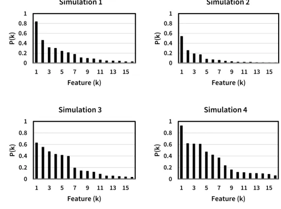
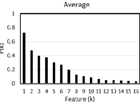
Since this stick-breaking process is stochastic, each application of the process will be random and unique, and so it is necessary to repeatedly simulate the process and average out across simulations in order to arrive at a reliable estimate of relative feature probabilities. Four generated simulations and their average are given in Figure 2.9.

Fig. 2.9. Four sample feature probability distributions generated by the

Stick-breaking construction (Teh et al., 2007) and their average given α=5.01, K=16.

0 0.2 0.4 0.6 0.8 1

1 3 5 7 9 11 13 15

P(k) Feature (k) Simulation 1 0 0.2 0.4 0.6 0.8 1

1 3 5 7 9 11 13 15

P(k)

Feature (k) Simulation 4 𝜋1=

(20)

As hoped, we can see that applying the stick-breaking process generates an interpretable expected feature probability distribution without worrying about customer or feature order. However, this does not fit the heavy-tailed power-law distributions associated with preferential attachment effects since plotting the distribution on a log-log scale does not produce a linear result (see Figure 2.10).

Fig. 2.10. The IBP generates a stretched-tail exponential distribution associated with

sublinear preferential attachment processes as represented by the noticeable curve in the log-log plot.

Instead, this distribution constitutes an example of a stretched-tail exponential distribution which have been shown to be generated by sublinear (weaker than power-law) preferential attachment effects which are importantly also attested in network formation and other processes (de Blasio et al., 2007; Gabel & Redner, 2013; Jeong et al., 2003; Rocha et al., 2010; Newman et al., 2002; Tomassini & Luthi, 2007). Therefore, the lack of a power-law distribution (as is most frequently associated with preferential attachment) does not invalidate the IBP algorithm, but rather raises a future question of whether power-law generating rich-get-richer algorithms or stretched-tail exponential algorithms like the IBP better fit language feature data. However, current analysis only considers the latter since the IBP algorithm is readily

(21)

available, efficient, and operates in the framework of connecting classes (phon. patterns) to one or more features.

In the coming sections, the stick-breaking algorithm (Teh et al., 2007) given in (6) will be used to generate expected IBP feature frequency distributions to test whether feature

implementation in phonological patterns is indicative of an IBP-like model for generating new phonological patterns.

3. Language Structuring Effects – A Corpus Study

The first test posited for determining whether language exhibits the effects of a phonological activeness bias is whether frequency activeness distributions within natural languages are indicative of a preferential attachment process like those discussed in §2.4. Such an effect could reasonably be expected given evidence in §2.3 that inductive biases in acquisition can shape the typology and structure of languages (Moreton, 2008; Moreton & Pater, 2012; Pater & Moreton, 2012) and the demonstration that an algorithm for acquiring phonological patterns with preferential attachment effects, the IBP, predicts a consistent, observable end-state feature probability distribution as discussed in §2.4 and illustrated in Figure 2.9.

Therefore, this section details a corpus study conducted using P-Base (Mielke, 2008), a collection of 7318 documented phonological rules and phonotactic distributions across 629 languages, in which feature activeness distributions for 21 languages were tested for goodness of fit with an IBP model. As an alternative hypothesis, goodness of fit with a Uniform Distribution model will also be tested. The Uniform Distribution assumes that every feature has equal chance of being chosen by a new class regardless of how many times a given feature has been selected up to that point. Therefore, the Uniform Distribution assumes no preferential attachment effects. As will be demonstrated, the stretched exponential distributions generated by preferential attachment processes like the IBP consistently fit observed language distributions better than distributions associated with equal preference for features (no preferential attachment) like the Uniform Distribution.

3.1. Procedure and Methodology

3.1.1. Feature Extraction

The first step in the analysis was to gather a large sample of phonological rules and phonotactic distributions for as many and as diverse languages as possible so as to derive

(22)

PBase

Both of the aforementioned requirements were satisfied by the PBase corpus (Mielke, 2008) which is a large collection of 7318 documented sound patterns (phonological rules and phonotactic distinctions) distributed across 629 languages represented in the corpus. In addition to sound patterns, sound inventories are also documented for each of the 629 languages.

Additionally, all of the patterns in P-Base have been encoded by features representing the classes involved in the patterns.

The P-Base web interface4 allows the user to specify a feature system for the database to use when displaying the classes involved in a rule or distribution. Given widespread agreement regarding many of its features and its relatively high performance in Mielke’s (2008) comparison of feature systems (SPE can characterize 70.97% of observed classes), the SPE feature set

(Chomsky & Halle, 1968) was used in this analysis.

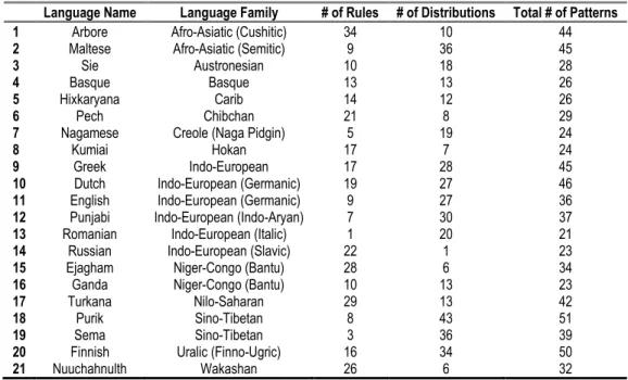
For the current study, the rules and distributions for 21 languages were parsed for phonologically active features. An attempt was made to include diverse representation of languages (13 distinct language families) and to avoid languages with few patterns to avoid confounds of a small sample size. To this end, a rule was established that only languages with 20 or more total patterns were considered. The languages are listed below alongside their family and the number of documented rules and distributions for each language (in P-Base):

Table 1. Languages Analyzed in the Corpus Study

Language Name Language Family # of Rules # of Distributions Total # of Patterns

1 Arbore Afro-Asiatic (Cushitic) 34 10 44

2 Maltese Afro-Asiatic (Semitic) 9 36 45

3 Sie Austronesian 10 18 28

4 Basque Basque 13 13 26

5 Hixkaryana Carib 14 12 26

6 Pech Chibchan 21 8 29

7 Nagamese Creole (Naga Pidgin) 5 19 24

8 Kumiai Hokan 17 7 24

9 Greek Indo-European 17 28 45

10 Dutch Indo-European (Germanic) 19 27 46

11 English Indo-European (Germanic) 9 27 36

12 Punjabi Indo-European (Indo-Aryan) 7 30 37

13 Romanian Indo-European (Italic) 1 20 21

14 Russian Indo-European (Slavic) 22 1 23

15 Ejagham Niger-Congo (Bantu) 28 6 34

16 Ganda Niger-Congo (Bantu) 10 13 23

17 Turkana Nilo-Saharan 29 13 42

18 Purik Sino-Tibetan 8 43 51

19 Sema Sino-Tibetan 3 36 39

20 Finnish Uralic (Finno-Ugric) 16 34 50

21 Nuuchahnulth Wakashan 26 6 32

(23)

Crucial Features

For each of the patterns in the languages above, the features used to denote the classes involved in each pattern were recorded. As mentioned in §1 and §2.4, features denoting rule inputs, environments, changes, and the classes involved in phonotactic distributions were recorded. Features denoting the output of a rule were not recorded since this is entirely predictable from all other information in the rule.

One caveat in the extraction of feature frequency data has to do with the algorithm P-Base uses to capture phonologically active classes as a set of features. Specifically, P-P-Base finds the minimum number of features needed to describe a class and then provides a list of all feature sets of that size which can capture the segments. Figure 3.1 is an example from a rule entry for Punjabi:

Fig. 3.1. Notice that there are two possible 3-feature descriptions of the class in the

environment 1 position. Both capture the class equally well without further data or some form of bias towards one class or the other. There are two crucial features, [back] and [high] which appear in both possible feature descriptions. Taken from P-Base (Mielke,

2008) Pattern 70265.

Assuming that language users restrict themselves to the simplest possible generalization of a class (see §2.2 for a discussion of complexity biases), learners must therefore use one of the feature sets utilizing the fewest features, but there is no obvious way to know which

characterizations speakers choose or whether all speakers consistently choose just one. To get around this issue, features were only counted when they were observed to be crucial to a class characterization, appearing in every possible feature set denoting a class. For example, [high] and [back] are crucial features for the environment 1 class in Figure 3.1.

This kind of analysis does drastically reduce the amount of data to be gained from the patterns in P-Base, but until some means of capturing which class characterization a language

(24)

user chooses is found, this is the safest form of analysis. In Table 2, the total number of crucial features found for each language in rules and distributions is listed.

Table 2. Number of Crucial Features per Language

Language Name in Rules in Distributions Total Crucial Features

1 Arbore 209 6 215

2 Maltese 26 118 144

3 Sie 62 23 85

4 Basque 76 12 88

5 Hixkaryana 93 12 105

6 Pech 141 21 162

7 Nagamese 16 13 29

8 Kumiai 80 5 85

9 Greek 84 21 105

10 Dutch 51 30 81

11 English 32 44 76

12 Punjabi NA NA 23

13 Romanian 0 25 25

14 Russian NA NA 14

15 Ejagham 57 19 76

16 Ganda 37 17 54

17 Turkana 106 18 124

18 Purik NA NA 49

19 Sema 12 42 54

20 Finnish 119 30 149

21 Nuuchahnulth 57 7 64

In Table 2, one can see that only counting crucial features still results in a large sample from which to estimate feature activeness distributions for each language with the possible exception of Russian which exhibited only 14 cases of crucial features across all rules and distributions. Nevertheless, Russian is not excluded from analysis since each language is tested separately for preferential attachment, and its inclusion has no danger of tampering with results for any other languages.

(25)

Fig. 3.2. The top plot shows English features ordered from most active (most frequent) to

least active and broken down by pattern type (rule or distribution) to show makeup of the total frequency. The bottom plot removes the “rule” and “distribution” bars to ease visualization of the distribution.

3.1.2. Model Fitting

With an observed feature activeness distribution constructed for all 21 languages, the next step was to find the IBP distribution (§2.4.1) and Uniform Distribution that most closely fitted each observed language distribution. In order to do this, a normalizing transformation was first applied to every language distribution and every candidate, IBP Distribution, and Uniform Distribution so that the summed bar height across all features added up to 1, now representing proportions rather than frequency. Then, for the IBP a brute force method of finding the best-fit IBP by generating every predicted IBP distribution from α=0.01 to α=10 with Δα=0.01 was used. The predicted IBP distribution for each α setting was the average of 1000 normalized sample simulations of Teh et al.’s (2007) stick-breaking process.

0 2 4 6 8 10 12 14 16 A c ti v en es s ( F req ue nc y ) Feature

English Feature Activeness Distribution

Total Count 0 2 4 6 8 10 12 14 16 A c ti v e n e s s ( Fr e q u e n c y ) Feature

English Feature Activeness Distribution

(26)

The predicted Uniform Distribution was derived by running 1000 simulations where each simulation involved randomly sampling one feature from the set of features until the number of total feature-uses in the language distribution was matched, and then ordering features from greatest to least number of times sampled. Then, like with the IBP, averaging across these 1000 sample simulations yielded the prototypical Uniform Distribution against which the language data was compared. Running this analysis results in a distribution as pictured in Figure 3.3. on the next page:

Fig. 3.3. (Left) Normalized Uniform Distribution generated from 1000 simulations with

100 samples across 15 features. For each simulation, features are ranked by number of times sampled from greatest to least, and averaging across the 1000 resulting

simulations gives the distribution seen below. (Right) Normalized IBP with 1000 simulations across 15 features with α=5.01.

In order to quantify the closeness of fit between each candidate model distribution (IBP and Uniform) and the observed language distribution, the sum of squared differences across all features was calculated and a smaller sum indicated a closer fit (Wellek, 2010).

(7) Sum of Squared Differences (d2₎

d2 = ∑𝐾_𝑘=1[𝐸(𝑘) − 𝑂(𝑘)]2

Therefore, the minimum sum of squared differences between the observed language distribution and each of all of the candidate IBP distributions indicates the best fitting IBP candidate. The d2 value for this IBP Distribution could then be compared to that of the generated Uniform

(27)

Fig. 3.4. The fit between the expected and observed distributions is equal to the sum of

the squared differences in proportion (height of the red lines) for each feature. Maximizing the fit means reducing differences between the expected and observed distribution, reducing the length of the red lines towards 0.

3.1.3. Calculating Likelihood of Affiliation

As mentioned previously, the goal of this corpus study is to show that languages exhibit distributions in their use of features in phonological patterns indicative of a phonological activeness bias with preferential attachment effects. This means, we need some way of

calculating the likelihood of that distribution actually being generated by an IBP-like process or a Uniform Distribution model, and the d2 value offered above is insufficient alone. This is because the IBP and Uniform Distribution models are stochastic processes which will return different results for each simulation even with the same parameters, hence the need to average out across 1000 simulations in generating best-fit candidate IBPs in the previous section.

These 1000 simulations not only coalesce to provide an estimate of the prototypical form of the IBP or Uniform model, but also provide an estimate of the range of variability in the manifestations of the process by calculating the d2 value between every simulation and the average and then constructing an empirical cumulative probability distribution for the d2 variable as shown in Figure 3.5.

Fig. 3.5. (Left) Empirical Cumulative Probability Chart for d2 variable for 1000 IBP simulations. As might be expected, there is a high-density interval of simulations with

small d2_{values which thins out as d}2_{increases and they differ more strongly from the}

mean. This distribution was generated for α=5.01 and K=16. (Right) ECPF for d2

variable for 1000 Uniform simulations with 100 samples each from 16 features (K=16).

0 0.05 0.1 0.15 0.2 0.25 0.3 0.35

1 2 3 4 5 6

P

(k

)

Feature (k)

Expected-Observed Fit Example

Expected

Observed

(28)

The distribution of d2_{values as seen in Figure 3.5 indicates that the simulations cluster}

around the mean and thin out as d2 increases. Given this knowledge, it is possible to put the hypothesis that languages implement an IBP process in other terms: The lower in the cumulative probability distribution that a language falls for the best-fitting IBP, the more likely it is that the language was a simulation of that process. Comparing this with its place in the d2 distribution for the Uniform model, we can see which provides a better fit of the language. Therefore, we are treating each observed language distribution as another simulation for the best-fitting IBP and the Uniform model, then finding its percentile in the cumulative probability distribution for each model as an indication of the likelihood of affiliation.

Fig. 3.6. (Left) The best-fit IBP (solid line) and Observed feature distribution (dotted

line) for English. (Right) Cumulative Probability Distribution for d2 for Best-Fit

simulations with red dot denoting the place of the observed language data in the

distribution. The same charts would be generated for the Uniform model and are shown in Figure 3.7.

Fig. 3.7.(Left) The Uniform (solid line) and Observed feature distribution (dotted line)

for English. (Right) Cumulative Probability Distribution for d2 for Uniform simulations

with red dot denoting the place of the observed language data in the distribution.

English Best-Fit IBP

(29)

3.2. Results and Interpretation

In Table 3, d2 values and percentile-scores for each candidate model (IBP or Uniform) are provided for each of the 21 languages considered in this study. Again, the lower the percentile-score, the better the candidate model in question fit the observed language data.

Table 3. Comparison of d2_{Percentile Scores for IBP and Uniform Distributions}

Language Name IBP d2_{Uniform d}2_{IBP percentile (%) Uniform percentile (%)}

1 Arbore 0.0004 0.0076 4.667 100

2 Maltese 0.0032 0.0244 37.167 100

3 Sie 0.0005 0.0086 0.833 99.967

4 Basque 0.0002 0.0016 0.833 86.433

5 Hixkaryana 0.0008 0.0038 17.667 99.633

6 Pech 0.0020 0.0468 6.9 100

7 Nagamese 0.0083 0.0690 11.467 100

8 Kumiai 0.003 0.024 33.467 100

9 Greek 0.0201 0.0917 53.767 100

10 Dutch 0.0175 0.0358 81.967 100

11 English 0.0006 0.0082 2.4 99.97

12 Punjabi 0.0078 0.0383 16.333 99.4

13 Romanian 0.0147 0.0475 41.033 99.999

14 Russian 0.0128 0.0191 54.2 92.633

15 Ejagham 0.0083 0.0234 60.867 100

16 Ganda 0.0014 0.0034 24.133 91.6

17 Turkana 0.0008 0.0291 1.633 100

18 Purik 0.002 0.0087 18.5 99.133

19 Sema 0.0027 0.0149 19.033 99.9

20 Finnish 0.0017 0.0086 40.033 100

21 Nuuchahnulth 0.0101 0.0217 69.6 100

(30)

Fig. 3.8.Languages are plotted by their IBP Percentile (x) and Uniform Percentile (y). The diagonal line divides the space into two regions with the upper region indicating better performance of the IBP distribution and the lower indicating better performance of the Uniform distribution. All analyzed languages favored the IBP and clustering in the lower percentiles (indicating a tight fit) is observable.

These results indicate that observed language distributions of feature use are consistent with the expected distributions emerging from a learning model implementing preferential attachment biases. Not only this, but a model assuming equal likelihood of using features like the Uniform Distribution fails to capture the observed distributions any better than the IBP, the lowest fit percentile being 86.433 in Basque. Together, these observations support the existence of a phonological activeness acquisitional bias on the basis of having found the distributions of feature-use in language structures expected to emerge over time.

4. Language Acquisition Effects – Artificial Language Task

Having found that language structures (feature activeness distributions) show evidence for a preferential attachment acquisition bias, the second component of this project tests for the effects of the bias on the learnability of phonological patterns utilizing phonologically active or inactive features. In other words, language grammars show the diachronic effect of phonological activeness biases, and we want to know whether language-users show the synchronic effect of showing preferential attachment to phonologically active forms. If the proposed bias is present, it is predicted that language learners should be more successful in acquiring patterns implementing highly active features. Given the ability to strongly control user input and to eliminate

confounds, an artificial language task in which participants learn artificial patterns through exposure to nonce word stimuli was selected to test for this effect. The experiment design is heavily inspired by that of Pater & Tessier (2006) who compared the learnability of artificial language sound patterns with and without phonotactic motivations in English.

0 10 20 30 40 50 60 70 80 90 100

0 10 20 30 40 50 60 70 80 90100

U ni for m Per c enti le IBP Percentile IBP vs. Uniform Fit

Comparison

Favors IBP

(31)

Fig. 4.1. Feature Activeness in English

For this experiment, 100 English-speaking participants were divided into two groups of 50, and one group learned a sound alternation triggered by front vowels ([+/- back] is highly active in English) while the other learned the same alternation triggered by high vowels ([+/- high] is relatively inactive in English). These two features were chosen to allow for minimal differences between the two patterns acquired by participants other than the triggering features. Height and Backness are both properties associated with vowels. Participant success in learning and applying the alternations correctly was tested. The experiment design will be discussed in detail in §4.1 and task distribution covered in §4.2. Results are discussed in §4.3. As a brief preview, results from this experiment indicate that participants better learned a sound alternation triggered by the more phonologically active of the two tested triggering features ([+/- back]), although the difference was not significant. Nevertheless, the trends support the prediction that patterns using active features are more readily learned, thereby providing acquisitional evidence of phonological activeness bias effects.

4.1. Design and Methodology

4.1.1. Participants

For this experiment, 100 native-speakers of English were recruited anonymously through Amazon Mechanical Turk to participate. Before beginning the task, each potential participant was given a screening questionnaire to ensure that they were above the age of 18, had been born and were currently residing in the USA, and were not proficient in another language. This allowed for the reduction of potential confounds such as differing feature activeness rates in non-SAE accents/dialects and language transfer from other languages affecting participant

performance. Participants were assigned randomly into one of two experiment conditions, the Active or Inactive condition. In the end, 50 participants completed the task in each condition.

0 2 4 6 8 10 12 14 16 A c ti v en es s ( F req ue nc y ) Feature

English Feature Activeness Distribution

(32)

4.1.2. Task

The overall purpose of the experiment was to compare the learnability of sound patterns triggered by active phonological features versus those triggered by inactive features in a

speaker’s language. Therefore, like Pater & Tessier (2006) participants completed an artificial language learning task in which there were exposed to nonce word stimuli that carried evidence for a simple sound alternation, “t” epenthesis at the beginning of a word. The sound alternation for the two groups of participants was identical in every aspect except the class of sounds that triggered the application of the alternation.

The Active-condition group was given nonce words for which word-initial t-epenthesis was triggered by word-initial front vowels. The Inactive-condition group was given nonce words for which word-initial t-epenthesis was triggered by word-initial high vowels. Participants listened to these words while viewing pictures of objects, and were told to try and pair the words and pictures together. To assess acquisition of the patterns, participants were tested on their ability to apply the pattern correctly via a forced choice task in which they had to choose between applying t-epenthesis to a given word. Participants were tested on their ability to apply the pattern both to the training words and to the novel stimuli.

It should be noted that while the current experiment tested a phonological alternation of word-initial vowels triggering word-initial epenthesis, Pater & Tessier (2006) tested word-final alternations, specifically t-epenthesis triggered by either a word-final lax or front vowel (to test the effects of English L1 phonotactics). There were two reasons for choosing prefixed plurals and word-initial alternations: 1) eliminate the possibility that participants believe t-epenthesis with lax-vowels like /ɛ/ to be triggered by English phonotactics rather than the rule against front or high vowels, 2) create a distinct pattern that English speakers would have little precedent for other than the features involved, thereby reducing possible advantage given to either pattern morphological knowledge or analogy to a similar pattern on any basis other than the features involved.

4.1.3. Stimuli

(33)

Table 4. Experiment Stimuli

Frontness (Active) Height (Inactive)

V-t [-back] V-no t [+back] C V-t [+high] V-no t [-high] C

P S P S P S P S P S P S

[vɑsik] [tik] [vɑsup] [up] [vɑskip] [kip] [vɑsik] [tik] [vɑsæt] [æt] [vɑskip] [kip] [vɑsip] [tip] [vɑsunt] [unt] [vɑskor] [koɹ] [vɑsip] [tip] [vɑsæl] [æl] [vɑskoɹ] [koɹ] [vɑsifɑ] [tifɑ] [vɑsuki] [uki] [vɑsnɑs] [nɑs] [vɑsifɑ] [tifɑ] [vɑsædu] [ædoo] [vɑsnɑs] [nɑs] [vɑsilow] [tilow] [vɑsulow] [ulow] [vɑsnug] [nug] [vɑsilow] [tilow] [vɑsænow] [ænow] [vɑsnug] [nug] [vɑsæt] [tæt] [vɑsɑp] [ɑp] [vɑstɑl] [tɑl] [vɑsup] [tup] [vɑsɛn] [ɛn] [vɑstɑl] [tɑl] [vɑsæl] [tæl] [vɑsɑks] [ɑks] [vɑstimi] [timi] [vɑsunt] [tunt] [vɑsɛθ] [ɛθ] [vɑstimi] [timi] [vɑsædu] [tædu] [vɑsɑli] [ɑli] [vɑsmɑɹ] [mɑɹ] [vɑsuki] [tuki] [vɑsɛgi] [ɛgi] [vɑsmɑr] [mɑr] [vɑsænow] [tænow] [vɑsɑpɑk] [ɑpɑk] [vɑsmid] [mid] [vɑsulo] [tulo] [vɑsɛpɑ] [ɛpɑ] [vɑsmid] [mid] [vɑsɛn] [tɛn] [vɑsut] [ut] [vɑslɛk] [lɛk] [vɑsut] [tut] [vɑsɑp] [ɑp] [vɑslek] [lɛk] [vɑsɛθ] [tɛθ] [vɑsun] [un] [vɑslɑdu] [lɑdu] [vɑsun] [tun] [vɑsɑks] [ɑks] [vɑslɑdu] [lɑdu] [vɑsɛgi] [tɛgi] [vɑsugɹ] [ugɹ] [vɑspæk] [pæk] [vɑsugɹ] [tugɹ] [vɑsɑpɑk] [ɑpɑk] [vɑspæk] [pæk] [vɑsɛpɑ] [tɛpɑ] [vɑsuni] [uni] [vɑspoɹi] [poɹi] [vɑsuni] [tuni] [vɑsɑli] [ɑli] [vɑspoɹi] [poɹi]

All stimuli were recorded with Praat software (Boersma, 2002) by the experimenter, a trained linguist, and a volunteer pronouncing the stimuli under supervision of the experimenter in a closed closet with heavy blankets hung on the walls. Mono recordings were made with a

Logitech H390 microphone at 44100Hz sampling frequency. Intensity across recordings was normalized by scaling intensity to 70dB for all recordings. Experimenter recordings were used in learning blocks, and volunteer recordings were used in testing blocks to ensure that participants were not memorizing unintentional acoustic cues in the data. As a note, /u/ was pronounced non-centralized as in languages like French so as to ensure that participants mentally classified it as a high back vowel.

4.1.4. Experiment Flow

In this section, the layout and flow of the experiment is covered. Broadly, this experiment consisted of two types of blocks, learning blocks and test blocks:

Learning Blocks: Participants are told that plurals are created by prefixing /vas-/ to the root. For each noun, they learn the plural followed by the singular. In these blocks, participants are presented pictures showing the plural/singular concept while listening to the recorded pronunciation of the associated stimuli. Each plural/singular pair will appear 3 times in these blocks. Stimuli in learning blocks were those pronounced by the

(34)

Fig. 4.2. Learning Block trial example. /ik/ = “apple”

Test Blocks: In these blocks, participants are tested on words to see how well they have learned the pattern of [t]-epenthesis. Like the learning blocks, participants will be shown the plural form of a word with audio pronounced by the volunteer and its associated object. Then, the participant will be shown the picture for the corresponding singular form, and will be asked to choose the correct singular from two recorded audio choices given. One choice implements [t]-epenthesis and the other does not. For V-t and V-no t stimuli, this meant the presence of word-initial [t] or not. For C stimuli, [t] replacing the initial consonant was the [t]-epenthesis alternative since pure epenthesis would create invalid English onsets. Each word is tested twice.