1161.pdf

CHARLES W. KINSEY. Dosimetry of Custom Inserts for Electron

Beams Produced by a Varian Clinac 1800: Effect on Dose

Output and Mean Incident Energy.

Customizing of electron beam treatment dimensions is a

common clinical technique. The degree in which the measured

energy and dose output for a particular beam varies depends

on the degree of blocking and the nominal energy of that

beam. Published measurements for the Varian Clinac 1800 are

sparse and measurements for each custom insert manufactured

are time consuming.

Relative output and mean incident energy measurements

were performed for 160 nominal beam energy / cone / insert

combinations on a Varian 1800 at the Rock Hill Radiation

Therapy Center in Rock Hill, South Carolina.

Relative output measurements of the manufacturer sup¬

plied cones indicated no consistency in the data for all

nominal beam energies. For example, the variation in rela¬

tive output for increasing treatment field dimensions for

the 6 MeV beam is different than for the 20 MeV beam. For

custom square inserts within each cone, however, the data

presented consistent behavior for all beams. The "square

root" model for approximating relative output worked well

with the custom square inserts and rectangular inserts with

a relatively low length to width ratio. For rectangular

t.

inserts with a high length to width ratio, the model exhib¬

ited a positive bias for all nominal beam energies and

cones. It is theorized this bias may be due to the need to

extrapolate the measured data for very small dimensions. By

using some alternative measurement technique for these

smaller dimensions, the bias may be reduced to an acceptable

level.

The resulting energy measurements using the manufactur¬

er supplied cones and inserts were mimicked by the use of

custom inserts defining the same square dimensions for each

cone. These data showed no effect of the inserts / cones on

mean incident energy for the 6 MeV, 9 MeV, and 12 MeV nomi¬

nal beam energies. An effect on mean incident energy for

the 16 MeV and 20 MeV beams was noted only for the cases of

the 4x4 and 6x6 inserts and for cases of rectangular inserts

with a high length to width ratio. The "square root" model

for approximating mean incident energy appeared to be a

valid predictive tool for these measurements.

CONTENTS

List of Tables... vi

List of Figures...vili

1.0 INTRODUCTION ... 1

1.1 Clinical Use of Electron Beams ... 1

1.2 Varian Cllnac 1800 Electron Beam

Production ... 1

1.3 Custom Shaping o£ the Electron Beam... 4

1.4 Beam Characteritics Definitions ... 4

1.4.1 Dose Output and Relative Output .... 5

1.4.2 Mean Incident Energy... 7

1.5 Study Criteria Limits ... 8

1.5.1 Relative Output ... 9

1.5.2 Mean Incident Energy... 10

1.6 Study Objectives ... 10

2.0 MODEL DEVELOPMENT ... 12

2.1 AECL Therac 20 Electron Beam Production ... 12

2.2 Relative Output Model ... 12

2.3 Mean Incident Energy Model... 13

2.4 AECL Therac 20 and Varian Clinac 1800

Comparison... 14

3.0 MEASUREMENT METHODS ... 16

3.1 Study and Measurement Equipment ... 16

3.2 Relative Output Measurements ... 19

3.3 Mean Incident Energy Measurements ... 21

4.0 RESULTS... 23

4.1 Data Combinations... 23

4.2 Relative Output Measurements ... 23

4.3 Mean Incident Energy Measurements ... 32

4.4 Model Application ... 36

5.0 DISCUSSION... 67

5.1 Relative Output... 67

5.2 Mean Incident Energy... 71

5.3 Current Model Developments ... 72

6.0 SUMMARY...75

7.0 CONCLUSION...77

Appendix A...79

Appendix B...89

LIST OP TABLES

Table

1 Comparison between the Therac 20 and

the Clinac 1800...15

2 Applicators supplied by Varian ... 17

3 Custom Inserts manufactured ... 18

4 Varian Cones: Relative output ... .24

5 Custom square inserts: Relative output ... 26

6 Custom rectangular inserts: Relative

output...33

7 Varian cones: 50% of maximum ionization

depth...34

8 Custom square inserts: 50% of maximum

ionization depth ... 37

9 Custom rectangular inserts: 50% of

maximum ionization ... 43

10a 6 MeV: Relative output - A comparison .... 46

10b 9 MeV: Relative output - A comparison .... 48

10c 12 MeV: Relative output - A comparison .... 50

lOd 16 MeV: Relative output - A comparison .... 52

lOe 20 MeV: Relative output - A comparison .... 54

11a 6 MeV: 50% Maximum Ionization - A

comparison...56

lib 9 MeV: 50% Maximum Ionization - A

comparison...58

lie 12 MeV: 50% Maximum Ionization - A

comparison...60

lid 16 MeV: 50% Maximum Ionization - A

comparison...62

12 Rbo to R«B (or Rbs) Difference...66

13 Relative Output Prediction Summary ... 68

14 Mean Incident Energy Prediction Summary .... 73

Figure

1 Varian Clinac 1800: A simplified diagram ... 3

2 Varian Cones: Relative output ... 25

3 6x6 Cone: Relative output ... 27

4 10x10 Cone: Relative output ... 28

5 15x15 Cone: Relative output ... 29

6 20x20 Cone: Relative output ... 30

7 25x25 Cone: Relative output ... 31

8 Varian Cones: 50% of maximum ionization

depth...35

9 6x6 Cone: 50% of maximum ionization

depth...38

10 10x10 Cone: 50% of maximum ionization

depth...39

11 15x15 Cone: 50% of maximum ionization

depth...40

12 20x20 Cone: 50% of maximum ionization

depth...41

13 25x25 Cone: 50% of maximum ionization

depth...42

14 Comparison of % Pass vs. increasing

criteria limits ... 70

1.0 INTRODUCTION

1.1 Clinical Use of Electron Beams

Microwave-powered electron linear accelerators have

become a popular tool for the treatment of cancer in the

practice of radiation therapy. One class of these accelera¬

tors, known as high energy medical linacs, can deliver x-ray

beam(s) of either single or dual energy and electron beams

of multiple energies over a relatively broad surface area.

Electron beams with their high surface dose delivery

and characteristically sharp dose fall-off with depth are

ideal for the treatment of relatively superficial tumors

such as skin lesions, cancers of the head and neck area, and

postoperative breasts and chestwalls.(10) It has been

estimated that electron beam therapy is indicated as either

the primary mode or as an adjunct to x-ray treatment for

approximately 10% of the patients treated in a radiation

therapy clinic.(10)

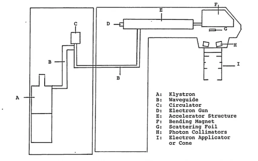
1.2 Varian Clinac 1800 Electron Beam Production

One model of linear accelerator that generates dual

x-ray energies and five electron energies and is the subject

Asso-acceptable electron beam by the following (see Figure 1):

First, a stream of electrons is introduced by an

"electron gun" into a klystron powered accelerator

guide which will generate a current of an average

specified energy.

Second, this current enters a bending magnet which

produces a coarse steering of the electron current

and behaves as a discreet energy window for the

electrons.

Third, the steering of the electron current exit¬

ing the bending magnet is more finely adjusted by

electromagnetic steering coils so the electrons

will impinge onto a scattering foil. The interac¬

tion of the electron current with the scattering

foil generates a broad electron beam.

Fourth, this broad beam is first collimated or

shaped by interleaved x-ray collimators. Second¬

ary collimation is then performed by an attachment

made of a fiberglass frame with aluminum baffles

at varying distances from the source and a steel

insert located at the exit end of the attachment.

This insert defines the actual dimensions of the

electron beam produced for clinical use.

The manufacturer supplies a group of these attachments,

called applicators or cones. Each cone in combination with

B

L

B

Q O-h-E

Klystron

Waveguide

Circulator

Electron Gun

Accelerator Structure

Bending Magnet

Scattering Foil

Photon Collimators

Electron Applicator

or Cone

.'

ͣ

fV-^Y ;!

Figure 1. Varian Clinac 1800: A simplified schematic diagreun indicating

the major components discussed in the text.

One difficulty with attempting clinical use with only

these square dimension inserts is that cancerous tumors very

rarely are shaped as squares. A mechanism is available for

the user to manufacture custom shaped inserts using a high-Z

metal alloy and attach them to the supplied cones to custom¬

ize the treatment field to the individual's case. This

allows the clinician greater flexibility in sparing non¬

cancerous regions on / in the patient.

A possible uncertainty in treatment is introduced by

using these custom inserts. The placing of a custom shaped

slab of high-Z material into the electron beam's path to

modify the treatment field dimensions may measurably affect,

within the effective treatment field, the characteristics

used as criteria for clinically acceptable use. The possi¬

ble modification of beam characteristics by the use of

custom inserts is the subject of this study.

1.4 Beam Characterictics Definitions

Two of the characteristics used to indicate the accept¬

able clinical use of an electron beam are a measured ab¬

sorbed dose delivered or dose output and a measured mean

C 5

1.4.1 Dose Output and Relative Output

Dose output is defined as the absorbed dose (usually in

units of gray (Gy) or centigray (cGy)) delivered at a depth

of maximum dose build-up (D«««) within a measurement phan¬

tom. In practice, this measurement is taken at the central

axis of the beam with a National Bureau of Standards (NBS)

traceable calibrated ionization chamber and electrometer

combination. The collected ionization data is then convert¬

ed to absorbed dose by the application of an accepted cali¬

bration protocol. For this study, the AAPM TG-21 (American

Association of Physicist in Medicine Task Group 21) calibra¬

tion protocol is used.(11) With this protocol the ioniza¬

tion readings, corrected for atmospheric conditions, are

converted to absorbed dose in the phantom material or medium

by the expression

D^-MxN^x(L/p):!^xP,^xP^^j_ (1)

where Dm.<9 = the absorbed dose at Dm«j. in the phantom

medium,

M = the ionization reading,

Ng*. = the ion chamber's calibration factor,

(L/p)«ic"'"** = the restricted stopping power ratio,

Pion = the chamber ionization recombination cor¬

rection factor,

and PjT-px = the chamber replacement (electron fluence)

correction factor.(11)

If the phantom material is water, as is true in the present

study, Dm.ei = Dw«i=-B. If the phantom is not water, then the

(S/p)m«ca'"'*=•*' = the unrestricted stopping power

ratio,

and Om«<a"

ͣ

*=•'' = the electron fluence phantom correc¬

tion factor

is needed.(11)

Parallel plate ionization chambers in the accelerator

are used to continuously monitor the generated radiation.

The units of measurement for these chambers are designated

monitor units (MU). During accelerator calibration, the

electronics for these chambers are adjusted such that for a

designated defined field size (in this case 10 cm x 10 cm

dimensions) a dose output of 1.00 cGy/MU is measured in a

phantom at Dm««. For other field sizes or cones, the dose

output must be measured and is reported relative to the

designated field size. These dose outputs are called rela¬

tive outputs. TG-21 protocol does not specifically address

how these relative outputs should be measured which has

resulted in two basic techniques as to how these measure¬

ments are performed. One technique is that for each field

size the ionization measurements are performed at the depth

of maximum dose (i.e. Dm«>c} and the dose outputs are calcu¬

lated using equations 1 and 2. The other is to take ioniza¬

tion measurements at the depth of maximum ionization for

each field size and calculate ratios to the ionization

measurements obtained at the depth of maximum ionization for

the 1.00 cGy/MU designated field size discussed previously.

For this study, the measurement at maximum ionization depth

1.4.2 Mean Incident Energy

We have been using terms such as Dm.x without precisely

defining how it is found. Dm*x is found by initially ac¬

quiring an ionization intensity versus depth below surface

data set. This involves placing the probe at various depths

along the central axis of the beam and collecting ionization

data at each depth. These ionization data are then convert¬

ed to absorbed dose by the use of equations 1 and 2. The

resulting data set is called a percent depth dose (%DD)

curve. The depth at which the maximum absorbed dose occurs

is designated Dm«M. There is also a depth at which maximum

Ionization is measured. This depth is labeled Rxoo. It

should be noted by the reader that Rioo may or may not be

equal to Dm«„.

The depth at which the ionization intensity is reduced

to one-half of the maximum value is labeled Rso. The TG-21

protocol uses this value, when expressed in centimeters, to

calculate the mean incident energy (Eo) by the expression.

(11)

^-2.33-^X/25p. (3)

This mean incident energy value is used to acquire from

tables supplied with the protocol the restricted stopping

power ratios used in equation 1 and the unrestricted stop¬

ping ratios and the electron fluence correction values used

The constant 2.33 MeV/cm for equation 3 was obtained by

assunning plane-parallel, infinitely vide monoenergetic

electrons incident upon a seni-infinite water phantom.(11)

Some commercial software packages include table look-up

values for this *'constant** that is dependent upon the field

size of the beam. Using this table look-up method, two

electron beans of different field sizes with the exact sane

Rbo value could have different Be values. Since both calcu¬

lation techniques (i.e. 2.33 MeV/cm for all beans vs. a

seperate constant for each field size) are currently being

used by the medical physics community, it is felt that

reporting Ee values for each beam / insert combination in

this study could be a source of confusion that could either

mask or accentuate the effect of the insert. Therefore, the

Rbo value in units of centimeters for a specified nominal

beam energy with its selected insert will be used as the

energy measurement criteria for this study.

The term nominal beam energy will be used to identify

each beam by the labeled beam energy specified by the manu¬

facturer. An example of this would be that for the beam

with a nominal beam energy o£ 6 MeV (i.e. labeled by the

manufacturer) the mean incident energy is 4.9 MeV (i.e.

calculated by equation 3).

1.5 Study Criteria Limits

^ 9

with a custom Insert is to measure the mean incident energy

and relative output of the specified beam in a phantom with

the custom insert in place. This is a time consuming pro¬

cess and is difficult to schedule in a busy clinic before

patient treatment is started. The ability to predict both

when and by how much a custom insert affects a beam's rela¬

tive output and mean incident energy prospectively would be

of use clinically in the realm of increased quality of pa¬

tient care and increased task scheduling efficiency of

dosimetry personnel.

3,,$,1 PQlqtttvQ QqtPMt

It has been estimated that the uncertainty inherent in

measuring electron beam dose output is approximately one

percent.(6) A criterion previously used as to a clinically

acceptable predictive model for dose output relative to

actual measurements is that predicted value should be within

one percent of actual measured value.(7) This amount of

accepted uncertainty falls well within the recommended upper

limit of uncertainty for total dose delivery to a target

volume, which is usually taken at five percent.(4) For

acceptable model prediction of relative outputs compared to

measured data, we will use a criterion of one percent varia¬

1.5.2 Mean Incident Energy fR»«)

The uncertainty in energy measurements by using the Rbo

value is dependent on the type and dimensions o£ the mea¬

surement probe and the precision of measurement probe place¬

ment within the phantom. This will be discussed in section

3.0.

For this study, the variation limit for acceptable

model prediction will be set by one of two options. One, the

limit will be set to equal the estimated uncertainty of Rbo

measurement. Two, the limit will be set to equal the dif¬

ference in depth between the measured Rbo value and either

the measured Rss (i.e. 55% of maximum ionization depth) or

the measured R^b (i.e. 45% of maximum ionization depth)

values for that specific nominal beam energy. The choice of

which variation limit is applicable will be based upon which

criterion is the least restrictive.

1.6 study Oblectives

The purpose of this paper is two-fold. First, measure¬

ments of relative output and mean incident energy (Rbo) for

custom inserts that define varying treatment field dimen¬

sions will be presented to add to the relatively sparse

database for this type of information pertaining to high

energy Varlan accelerators. Second, the possible application

s: 11

that estimates both the effect on dose output and mean

incident energy for non-standard rectangular fields will

2.0 MODEL DEVELOPMENT

2.1 AECL Therac 20 Electron Beam Production

A model was presented by Mills, et al. (8) to predict

the dose output for rectangular shaped electron beam fields

for a Therac 20 Saturne accelerator manufactured by Atomic

Energy of Canada Limited (AECL). For this accelerator, the

beam of electrons exiting the accelerator structure is

spread into a broad beam with a scanning guadrapole magnet.

The collimation system is composed of primary interleaved

photon collimators and secondary collimators, called trim¬

mers. These trimmers are physically attached to the primary

collimators, therefore both sets open and close in synchro¬

nization. The primary collimators define a field dimension

5 cm greater than the trimmers at 100 cm from the source.(8)

2.2 Relative Output Model

For model development, the electron beam is assumed to

be made up of a collection of pencil beams. By using the

theory of multiple coulomb scattering for electrons, an

expression was developed (8) that describes the spreading of

these pencil beams from the scattering in air which begins

at the location of primary collimators. Assuming no energy

£ 13

secondary collimators, the following expression was devel¬

oped that predicts the dose output for a rectangular shaped

field. This expression which came to be called the

"square-root model" is

where C*'* » the dose output of a rectangular field of

X^y dimensions,

0**'** » the dose output of a square field with

side dimension X,

and 0'''* = the dose output of a square field with

side dimension ¥.(8)

Appendix A is a reproduction of the original article which

contains this equation's derivation (equation number 15).

This expression will be used as the predictive model to

estimate relative outputs for non-standard rectangular in¬

serts.

2.3 Mean Incident: Bnerqy (Rbq) Model

The same group of researchers presented an expression

to predict the beam energy in the form of percent depth dose

(%DD) for rectangular shaped fields.(3) This expression has

the same mathematical form as equation 4 and is given by

where DD>*'^ » the %DD of a rectangular field of

X,y dimensions,

DD>*..>* = the %DD of a square field with side

dimension X,

and DD^'" » the %DD of a square field with side

dimension Y.(3)

contains this equation's derivation (equation number 17).

This expression will be used as the predictive model to

estimate Rso for non-standard rectangular inserts.

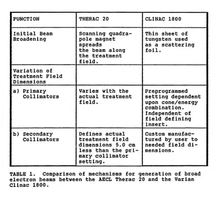
2.3 AECL Therac 20 and Varian Clinac 1800 Comparison

A possible difficulty with applying the previously

presented expressions to a Varian Clinac 1800 electron beam

is that its mechanism for the production of a broad electron

beam is different from the AECL Therac-20 Saturne for which

the model was developed. Table 1 compares some of differ¬

ences between the two accelerators. Even with these differ¬

ences noted, the present report focuses on the application

15

1 FUNCTION

THERAC 20

CLINAC 1800 1

ͣ

Initial Beam

Scanning quadra-

Thin sheet of 1

1 Broadening

pole magnet

tungsten used 1

spreads

as a scattering 1

the beam along

foil. 1

the treatment

field.

[variation of

1 Treatment Field

{Dimensions

la) Primary

Varies with the

Preprogrammed 1

1 Collimators

actual treatment

setting dependent 1

field.

upon cone/energy 1

combination. 1

Independent of 1

field defining 1

Insert. |

lb) Secondary

Defines actual

Custom manufac- 1

1 Collimators

treatment field

tured by user to 1

dimensions 5.0 cm

needed field dl- 1

less than the pri¬

mary collimator

setting.

menslons. 1

TABLE 1. Comparison of mechanisms for generation of broad

electron beams between the AECL Therac 20 and the Varian

3.0 MBASURBMEMT MBTHODS

3.1 Study and Measurement Equipment

The accelerator to which these measurements apply is a

Varian Associates' Clinac 1800 located at the Rock Hill

Radiation Therapy Center located in Rock Hill, South Caroli¬

na. This accelerator produces five electron beams with

nominal beam energies of 6, 9, 12, 16, and 20 MeV. Table 2

summarizes the field defining applicators or cones supplied

by the manufacturer with the nominal primary collimator

opening dimensions for each cone / energy combination.

A family of field shaping metal alloy inserts of square

and rectangular shape were made for each cone. The dimen¬

sions of the square inserts were chosen so that some would

mimic the defined field made by a smaller cone dimension.

One rectangular (i.e. length to width ratio greater than

one) insert with a small length to width ratio has side

dimensions that are bounded by the dimensions of the group

of custom square inserts for each specified cone. Another

rectangular insert with a large length to width ratio has

side dimensions that are larger and smaller respectively

than the dimensions of the group of custom square inserts

for each specified cone. Table 3 summarizes the actual

field defining inserts made for each cone.

manufac-17

1 APPLICATOR SIZE

COLLIMATOR SETTING |

6 AND 9 MeV

12, 16, and 20 1

MeV 1

4x4- 20x20

11x11 1

1 6x6-

20x20 11x11

10x10 20x20

14x14 1

1 15x15

20x20

19x19 1

1 20x20

25x25

25x25 1

1 25x25

30x30

30x30 1

Both inserts used with 6x6 cone.

TABLE 2. Applicator / cone sizes with Inserts supplied by

1 CONE

CUSTOM INSERT CONE

CUSTOM INSERT 1

1 6x6

4x4 20x20

4x4 1

5x5

6x6 1

4x5

8x8 1

3x6

10x10 1

15x15 1

1 10x10

4x4

10x17 1

6x6

3x23 1

8x8

6x8 25x25

4x4 1

3x11

6x6 1

8x8 1

1 15x15

4x4

10x10 1

6x6

15x15 1

8x8

20x20 1

10x10

10x23 1

8x11

3x28 1

3x17

TABLE 3. Custom inserts manufactured with a low melting

f 19

tured by MultiData Systems International Corp. was used.

This system consist of a 48 x 48 x 40 cm water phantom with

automated scanning mechanisms, two PTW model M2332 0.1 cc

ion chambers (cavity diameter = 0.35 cm), and a controller

which is an IBM AT-compatible desktop computer running

proprietary software with accompanying interface equipment.

Data acquisition is performed with this system by

first, through software manipulation, developing an "acqui¬

sition plan file" which will control the positioning within

the water phantom of one probe designated the "measurement

probe." The other probe is set in a fixed position in the

path of the beam and is designated the "reference probe."

All data collected are relative to readings of this refer¬

ence probe. This guards against dose output rate (i.e.

cGy/min.) fluctuations of the accelerator which could com¬

promise the data from measurement techniques involving the

continuous repositioning of the measurement probe in the

beam's path while radiation is being delivered. Collected

data are stored in a separate "study file" for mathematical

and / or graphical manipulation.

3.2 Relative Output Measurements

For each cone / insert / nominal beam energy combina¬

tion, relative output measurements were performed by col¬

lecting ionization data at Rxoo. This was accomplished by

First, manually set the center of the measurement

probe at both the center of the defined field and

at the water surface of the phantom which was

previously set at 100 cm from the "target** of the

accelerator.

Second, following the recommendation of Attix (l),

offset the probe 0.75 times the radius of the

probe's active volume (i.e. 0.1 cm) away for the

radiation beam "target" for all of the data mea¬

surement points. Set this position to be the

scanning origin of the water phantom.

Third, by computer keyboard control, move the

measurement probe to the previously determined

Rxoo depth (see Section 3.3) for a specified cone

/ insert / nominal beam energy combination.

Fourth, collect the signal from the measurement

probe with a PRM model SH-1 electrometer. This

will be the ionization data for that specific

combination.

Fifth, repeat the third and fouth steps until

ionization data for all cone / insert / nominal

beam energy combinations are acquired.

s: 21

values that were calculated by the following expression:

___ , lONIZATIOK READINGS) -^r ,^

icaazATim readings) ^qxio "'^

The 10x10 cone with Varian supplied insert combination

for each beam had been previously calibrated to a value of

1.00 cGy/MU at the depth of maximum dose (i.e. D»*m) with a

NBS traceable calibration dosimetry system. This system

consisted of the same PRM model SH-1 electrometer and a

Capintec model PR-06G Parmer-type probe.

3.3 Mgan Incident Energy (Rbq) MeasMcementg

For Rbo measurements, relative ionization versus depth

curves were acquired. This was performed for each cone /

insert / nominal beam energy by the following procedure:

First, manually set the center of the measurement

probe at both the center of the defined field and

at the water surface of the phantom which was

previously set at 100 cm from the "target" of the

accelerator.

Second, following the recommendation of Attix (1),

offset the probe 0.75 times the radius of the

probe's active volume (i.e. 0.1 cm) away for the

"target" for all of the data measurement points.

Set this position as the scanning orgin of the

water phantom.

the beam but not at a location that would inter¬

fere with the scanning mechanism.

Fourth, develop an acquisition plan that guides

the probe into the water phantom along the central

axis of the field at depth increments of 0.1 cm

and to an absolute depth past the effective range

of the electron beam's energy.

Fifth, with the system's electrometer time con¬

stant set at 0.2 seconds, have the probe pause 0.4

seconds at each depth increment or sampling point.

Sixth, enter the command to begin the acqusition

of the ionization intensity vs depth data.

The scanning system software will automatically display the

ionization intensity vs. depth scan normalized to the maxi¬

mum ionization value. A printout is then acquired which

contains depths of maximum ionization (Rioo), 50% of maximum

ionization (Rso), 55% of maximum ionization (Rss), and 45%

of maximum ionization (R419) values.

The combination of uncertainties in the previouly

described steps involved in probe positioning results in an

estimated uncertainty of 0.1 cm for the measured Rso value.

Therefore, one pass / fail criterion for Rso model predic¬

s." 23

4.0 RESULTS

4.1 Data Combinations

Relative output and ionization intensity versus depth

curves were measured for 180 nominal beam energy / cone /

insert combinations. Thirty combinations vere with Varlan

supplied Inserts, 100 combinations vere with custom square

inserts and 50 combinations vere vlth custom rectangular

Inserts.

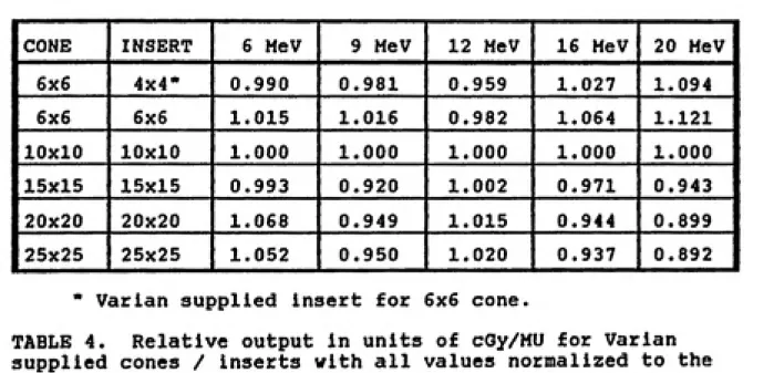
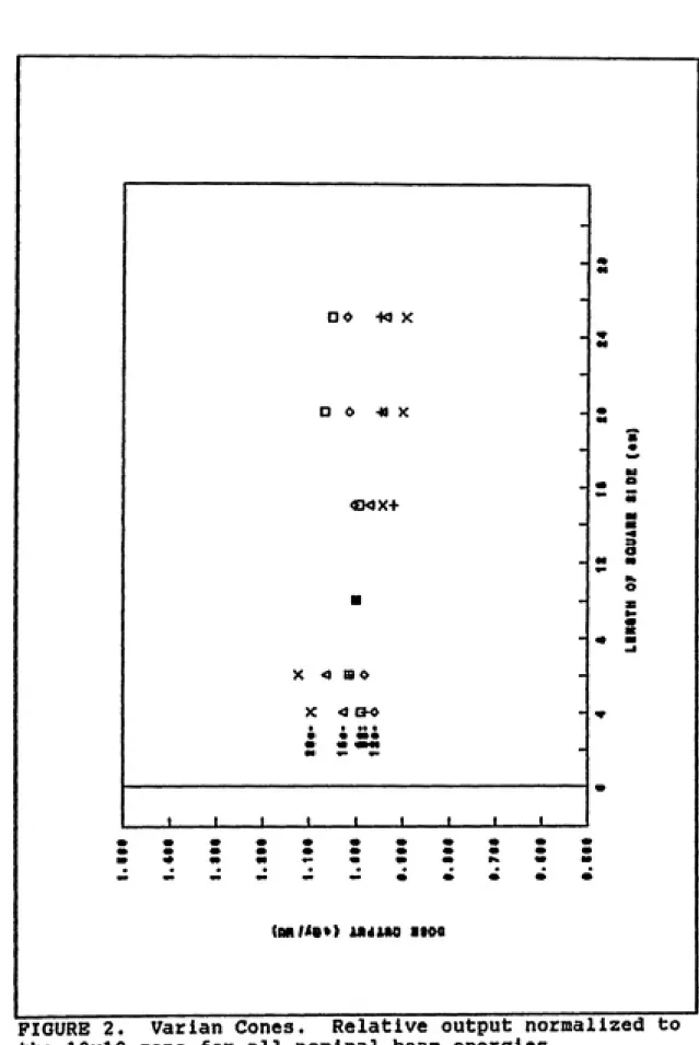
4.2 Relative Output Measurements

Table 4 presents the relative output measurements for

each nominal beam energy vith all cone / manufacturer sup¬

plied Inserts. Figure 2 presents these data graphically. A

reviev of this graph indicates no consistent shape of the

curves for all beams. This could be due to the different

primary collimators settings for different cone / beam

combinations and different construction dimensions for each

individual cone as indicated in table 2. Table 5 presents

the relative output measurements for all cone / square

insert / nominal beam energy combinations. Figures 3

through 7 graphically present these data for each beam. As

can be observed for these curves, there appears to be a

|cONB

INSERT 6 MeV 9 MeV 12 MeV 16 MeV

20 MeV 1

1 6x6

4x4* 0.990 0.981 0.959 1.027

1.094 1

16x6

6x6 1.015 1.016 0.982 1.064

1.121 1

110x10

10x10 1.000 1.000 1.000 1.000

1.000 1

115x15

15x15 0.993 0.920 1.002 0.971

0.943 1

120x20

20x20 1.068 0.949 1.015 0.944

0.899 1

125x25

25x25 1.052 0.950 1.020 0.937

0.892 1

* Varian supplied insert for 6x6 cone.

TABLE 4. Relative output in units of cGy/MU for Varian

supplied cones / Inserts with all values normalized to the

25

1

_

-

* 1

** 1

DO -W X

-s

DO -m X -

• 1

M 1

>> 1

• 1

CMX4

-•" S 1

M 1 MM 1 •• 1 Ik 1

e 1

ͣ

-s 1

^ 1

s

mm 1

^ 1

X O BO

-|

X < B-O J

V 1

ff t ffi i • • «•• • « «M«

« <• «-

-1

1 «

1 •

1 "

1 1 1 1 1 1 1 1 •

I « •» M «- • •» M

• • • • « •

» 1

» 1

> 1

1 m

', JiJitiJiml^m

•

•

•

•

ͣ

• 1

(Mlf««»> M4iM ItM

FIGURE 2. Varian Cones. Relative output normalized to

JCONE

INSERT 6 MeV 9 MeV 12 MeV 16 MeV

20 MeV 1

lexe

4x4V 0.990 0.981 0.959 1.027

1.094 1

4x4 0.982 0.980 0,948 1.016

1.064 1

5x5 1.012 1.013 0.960 1.036

1.082 1

6x6V 1.015 1.016 0.982 1.064

t ^-^21 1

110x10

4x4 0.962

_{^ 0.924}

0.956 0.968

0.966 1

6x6

; 1.001

0.990 0.992 0.992

0.990 1

8x8 0.996 0.998 0.995 0.995

0.991 1

lOxlOV 1.000 1.000 1.000 1.000

1.000 1

115x15

4x4 0.965 0.874 0.956 0.937

0.931 1

6x6 0.993 0.920 0.998 0.961

0.941 1

8x8 0.996 0.932 1.013 0.972

0.953 1

10x10 0.995 0.930 1.012 0.980

0.954 1

15xl5V 0.993 0.920 1.002 0.971

0.943 1

120x20

4x4 1.030 0.895 0.965 0.923

0.906 1

6x6 1.076 0.955 1.020 0.951

0.915 1

8x8 1.078 0.962 1.031 0.957

0.918 1

10x10 1.075 0.961 1.035 0.962

0.921 1

1 -.

_15x15 1.068 0.956 1.029 0.958

0.919 1

20x20V

1.068 0.949 1.020 0.944

0.899 1

125x25 1

4x4 1.017 0.904

0.979 1

0.934

0.913 1

6x6 1.067 0.966 1.037 0.966

0.940 1

8x8 1.072 0.974

1.047 1

0.973

0.939 1

1

10x10 1.071 0.974

1.049 '

0.969

0.932 1

15x15 1.064

0.964 J

1.040

0.966

0.924 1

20x20 1.059 0.954 1.028

0.951 !

0.907 1

25x25V

1.052 0.950 1.020 0.937

0.892 1

TABLE 5. Relative output

square inserts and Varian

10x10 cone.

27

X 4 BO

X *m o

XX 4)B<»

• • «ͣ •

I I I_____I_____I---1_____I_____L

• S •

* # *

UMfAl*) ia^JUM IIM

FIGURE 3. 6x6 Cone. Relative output normalized to the

<•«»<••) U4AM Itoa

FIGURE 4. 10x10 Cone. Relative output normalized to

29

CMX-I-<09X4 <04K4

+

Ha •

J_____\ \_____L J_____L

s

8

(Mlf4«t) M4iM IMA

1

M

M

a 0 •« X •«•

• 1

O 0 4 X

•

m

8

5 1

ͣ

1

* 1

o « « X

K 1

1

ͣͣ

1

i^ 1

O « -MX «

O O -MX

a o 4«- »

• • • t*

1 1 1 1 1 1 1 1 1

1 «

1 «

1 n

; s 8 s s s : :

•

•

:

1

• 4» •

\mit%%} AaiiM ͣ•»•

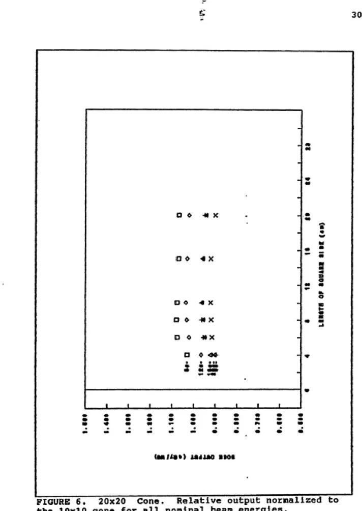
FIGURE 6. 20x20 Cone. Relative output normalized to

31

s

O* +« X

* 1

_{«ͣ 1}

o» -m X

4» 1

M 1

• 1

DO 4 X

4 1 ^ 1 OO « X

oo «x DO «X

D 9 4»«>

« 1

• • I M

1 «

1 4

1 ͣ

1 1 t t 1 1 1 I i

• •

• •

» 1

» 1

> 1

..»«ͣ•*• • •

• 1

(Mli«»> AII4AM BM«

each individual cone.

For the 15x15 cone and greater (figures 5 through 7),

this trend can be described as follows:

A maximum output is observed between the 8x8 and

10x10 inserts. With increasing square field di¬

mension, the relative output changes in a linear

fashion with a slight negative slope of approxi¬

mately -0.002 cGy/HU per cm of square side dimen¬

sion. With decreasing square dimensions, a much

sharper (3% to 6%) non-linear drop in output is

observed.

The non-linear trend for smaller square dimensions is mim¬

icked to a lesser degree in the 10x10 and 6x6 cone. One

abnormality for the 6x6 cone was an apparent difference

(especially for the higher energies) in output between the

Varian supplied 4x4 insert and a 4x4 custom made insert.

The data for the 4x4 and 5x5 custom inserts were used for

relative output model prediction with non-standard custom

rectangular inserts.

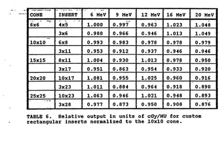
Table 6 presents the relative output measurements for

the two rectangular custom inserts used in the present study

for each cone / nominal beam energy combination.

4.3 Mean Incident Energy (RboI

Table 7 presents mean incident energy (Rbo) measure¬

33

|COME

INSERT

1 6 MeV

9 MeV 12 MeV 16 MeV

20 Mev|

Isxe

4x5 1.000 0.997 0.963 1.023

1.048 1

3x6 0.980 0.966 0.946 1.013

1.049 1

110x10

6x8 0.993 0.983 0.978 0.978

0.979 1

3x11 0.953 0.912 0.937 0.946

0.946 1

115x15

8x11 1.004 0.930 1.013 ͣ 0.978

0.950 1

3x17 0.951 0.863 0.954 0.933

0.920 1

120x20

10x17 1.061 0.955

1.025

0.960

0.916 1

3x23 1.011 0.884 0.964 0.918

0.890 1

125x25

10x23 1.063 0.946 1.021 0.948

0.893 1

3x28 0.977 0.873 0.950 0.908

0.876 1

1 COMB

INSERT 6 MeV 9 MeV 12 MeV 16 MeV

20 Mev|

1 6x6

4x4* 2.2 3.4 4.3 5.7

6.6 1

1 6x6

6x6 2.2 3.4 4.5 6.1

7.4 1

1 10x10

I 10x10

2.1 3.3 4.5 6.4

7.8 1

I 15x15

15x15 2.2 3.4

1 4.5

6.3

7.8 1

I 20x20

20x20 2.2 3.4 4.5 6.4

7.9 1

1 25x25

,25x25

2.1 3.4 4.5 6.4

7.9 1

* Varian supplied insert for 6x6 cone.

TABLE 7. 50% of the ttaximuA ionization depth in centiaeters

35

-1

H

X 4 ^ + O

-]

X 4 ^ + O

-1

X 4 « + D

-1

X 4 0 + O

A

X 4 « + D

J

X 4 o + ͤ J

ͣ

t • • • •

•

•

M

• 1

•

•

4

...i... ...In,,.. 1. ..,.,1...i...1 ____L- 1 i

i

. s

8

!

ͣ

•) HOIiVXMOl MMIIXVII %«t

FIGURE 6. Varian Cones. 50% of naximun ionization

combinations. Figure 8 presents thes data graphically. As

can be seen, for the 6 MeV, 9 MeV, and 12 MeV nominal beam

energies, the Rbo value remains constant for all combina¬

tions. For the 16 MeV and 20 MeV nominal beam energies,

these data indicate a Rao value decrease for the 6x6 cone

vith the 6x6 and 4x4 inserts.

Table 8 presents the mean incident energy (Rso) mea¬

surements for each cone vith their respective families of

custom inserts. Figures 9 through 13 graphically present

these data for each beam. A review of these graphs indicate

a Rso value decrease for the 16 MeV and 20 MeV nominal beam

energies with the 10x10 and greater dimension cones' 4x4 and

6x6 inserts. This Rso decrease for the smaller inserts is

qualitatively similar to that noted earlier with the cone /

manufacturer supplied inset combinations. The 6 MeV, 9 MeV,

and 12 MeV nominal beam energies' data are constant for all

inserts which is again comparable to data for the individual

cones.

Table 9 presents mean incident energy (Rbo) measure¬

ments for the two rectangular custom inserts used in the

present study for each cone / nominal beam energy combina¬

tion.

4.4 Model Application

For application of the square root model for both

predic-37

1 CONE

INSERT 6 MeV 9 MeV 12 MeV 16 MeV

20 Mev|

1 6x6

4x4V 2.2 3.4 4.3 5.7

6.6 1

4x4 2.2 3.3

1 4.4

5.8

1 6.8 1

5X5 2.1 3.3 4.4 6.2

7,3 1

1 6x6V

2.2 3.4 4.5

1 6.1

7.4 1

1 10x10

4x4

\ 2.1

3.3 4.3 5.9

6.8 1

1 6x6

I ^'^

3.3 4.5 6.3

7.6 1

8x8 2.1 3.3 4.5 6.4

i ^'^ i

1

1 lOxlOV

2.1 3.3 4.5 6.4

1 7.8 1

1 15x15

4x4 2.2 3.4 4.4 6.0

7.0 1

1

6x6 2.2 3.5 4.6 6.3

7.6 1

8x8 2.2 3.5 4.6 6.3

7.7 1

10x10 2.2 3.5 4.6 6.3

7.8 1

1

15x15V

2.2 3.4 4.5 6.3

7.8 1

1 20x20

4x4 2.1 3.3 4.3 5.9

6.9 1

6x6 2.1 3.4

4.5 1

6.3 1

7.6 1

8x8 2.1

3.4 i

4.5 6.4 i

7.8 1

10x10 2.1 3.4 4.5 6.5

7.8 1

15x15 2.2 3.5 4.5 6.4

7.8 1

20x20V 2.2 3.4 4.5 6.4

7.9 1

I 25x25

4x4 J

2.1 3.3 4.3

5.8 J

6.9 1

1

6x6 1

2.1 1

3.4

4.5 1

6.3

7.7 1

8x8 1

2.2

3.4 '

4.5 6.4

8.0 1

10x10 2.2 3.4 4.5 6.4

8.0 1

15x15

2.2 3.5 4.6 6.5

8.1 1

1 ͣ" ͣ !

20x20

2.1 3.4 4.5 6.3

7.9 1

25x25V

2.1 3.4 4.5 6.4

7.9 1

TABLE 8. 50% of aaxinum i

all square custom inserts

onization depth in centimeters for

Hit) iOliVXMOl RMtXVR »«t

PIGURB 9. 6x6 Cone. 50% o£ naxinum ionization depth

.39

X 4

X 4

X < X 4

O « «

+

+

+

o o D O

• •

J_____I_____1_____I_____I_____I_____I I I

s

m

- 6

8

(

ͣ

•> MIAVZIIiOl IMIIIXVa «M

FIGURE 10. 10x10 Cone. 50% o£ maxinua ionization depth

K <

X <

X 4

X 4

•

4 4

4

4 a o D O

J_____L J_____L

i

•• A

!

!

ͣ

•> lOUVIIIOI HMIXm KM

FIGURE 11. 15x15 Cone. 50% o£ naxi»un ionization depth

.41

»•> MOIAVIIiOl NMIKVR ««t

FIGURE 12. 20x20 Cone. 50% of maxiKua ionization depth

-]

X 4 ^ + o

-j

X < 6 + o

-1

X < 0 + o

-|

X 4 0 + o

-j

X 4 ' o 4 ͣ o

-1

X « + D

-1

X < 0 + O J

• • • •

t • «

I •

• 1

•

•

4

1 .. , L... 1 1 1 1 1 i

1 t

4

8

lit) MUVIIiOl RMixvn «u

FIGURE 13. 25x25 Cone. 50% o£ maxinlin ionization depth

43

|C0MB '

INSERT 6 MeV

_{i 9 MeV}

! 12 MeV

16 MeV

\ 20 Mev|

1 6x6

4x5 2.1 3.3 4.4 5.9

6.9 1

3x6 2.1 3.2 4.3

1 ^*^

6.7 1

1 10x10

1 6x8

2.2

1 3.3

4.5

1 ^'^

1 ^'^ 1

3x11 2 .^ : 3.3

i *'*

5.9

6.9 1

1 15x15

8x11 2.2 3.4

\ *'^

6.4

7.8 1

1

3x17 2.2 3.4 4.4 5.9

7.0 1

1 20x20

10x17 2.2 3.4 4.5 6.4

7.9 1

3x23 2.2 3.4 4.4 5.9

7.1 1

1 25x25

10x23 2.2 3.4 4.5 6.4

7.9 1

1

3x28 2.2 3.4

_{1 *'*}

6.0

7.1 1

TABLE 9. 50% o£ maximum ionization depth in centimeters for

tion, a simple table look up algorithm was developed with

linear interpolation for field defining dimensions between

table values and linear extrapolation for field defining

dimensions outside the table values. Examples of this

algorithm are:

Bxample 1 - Relative output prediction using linear

interpolation and equation 4.

Cone: 20 cm x 20 cm

Beam: 16 HeV

Table: lOd

Insert: 10 cm x 17 cm

Qxomxy (measured) = 0.960 cGy/MU

0»««»«-0.962 coy/IflJ

Qi7jrtT. 0.952 c^/|«7

pmar . qUjos^

(^^'''0.951 cay/MU

Example 2 - Energy (Rbo) prediction using linear ex¬

trapolation and equation 5.

Cone: 20 cm x 20 cm

Beam: 16 MeV

Table: lid

Insert: 3 cm x 23 cm

!* 45

SD^*'" S .f cm

i»»»*»*-6.4caB

Tables 10a through lOe present comparisons between the

measured and predicted values of the relative output for all

square and rectangular inserts for each cone and for each

nominal beam energy, 6 MeV through 20 MeV respectively.

Tables 11a through lie present comparisons between the

measured and predicted values of Roo for square and rectan¬

gular inserts for each cone and for each nominal beam ener¬

gy, 6 MeV through 20 MeV respectively.

Table 12 contains the variation in depth values between

measured Rbo and measured R^b (or Rbb) for each nominal beam

energy. These data are to be used as a possible pass / fail

1 Cone

Insert Cone Model Cone

Mode 1

Meas. Pred. Pred. %Diff.

%Diff. 1

1 6x6

4x4V 0.990 0.990 0.990 0.0%

0.0% 1

6x6V 1.015 1.015 1.015 0.0%

0.0% 1

4x4 0.982 0.990 0.982 0.8%

0.0% 1

5x5 1.012 1.015 1.012 0.3%

0.0% 1

4x5 0.997 1.015 0.997 1.8%

0.0% 1

3x6 0.980 1.015 0.997 3.6%

1.7% 1

10x10 4x4 0.962 1.000 0.962 3.9%

0.0% 1

6x6 1.001 1.000 1.001 -0.1%

_{0.0% 1}

8x8 0,996 1.000 0.996 0.4%

0.0% 1

lOxlOV 1.000 1.000 1.000 0.0%

0.0% 1

6x8 0.993 1.000 0.998 0.7%

0.5% 1

3x11 0.953 1.000 0.972 4.9%

2.0% 1

15x15 4x4 0.965 0.993 0.965 2.9%

0.0% 1

6x6 0.993 0.993 0.993 0.0%

0.0% 1

8x8 0.996 0.993 0.996 -0.3%

0.0% 1

10x10 0.995 0.993 0.995 -0.2%

0.0% 1

15xl5V 0.993 0.993 0.993 0.0%

0.0% 1

8x11 1.004 0.993 0.995 -1.1%

-0.9% 1

3x17 0.951 0.993 0.972 4.4%

2.2% j

TABLE 10a. 6 MeV: Relative Output. Comparison between

model prediction, assumption of no effect (cone), and actual

measurement for Varian and custom inserts. All absolute

values are in units of cGy/MU.

NOTE:

^Dlff

47

1 Cone

Insert Cone Model Cone

Mode 1

Meas. Pred. Pred. %Diff

%Diff 1

1 20x20

4x4 1.030 1.068 1.030 3.7%

0.0% 1

6x6 1.076 1.068 1.076 -0.7%

0.0% 1

8x8 1.078 1.068 1.078 -0.9%

0.0% 1

10x10 1.075 1.068 1.075 -0.6%

0.0% 1

15x15 1.068 1.068 1.068 0.0%

0.0% 1

20x20V 1.068 1.068 1.068 0.0%

0.0% 1

10x17 1.081 1.068 1.071 -1.2%

-0.9% 1

3x23 1.011 1.068 1.037 5.6%

2.6% 1

1 25x25

4x4 1.017 1.052 1.017 3.4%

0.0% 1

6x6 1.067 1.052 1.067 -1.4%

0.0% 1

8x8 1.072 1.052 1.072 -1.9%

0.0% 1

10x10 1.071 1.052 1.071 -1.8%

0.0% 1

15x15 1.064 1.052 1.064 -1.2%

0.0% 1

20x20 1.059 1.052 1.059 -0.6%

0.0 1

25x25V 1.052 1.052 1.052 0.0%

0.0% 1

10x23 1.063 1.052 1.063 -1.0%

0.0% 1

3x28 0.977 1.052 1.020 7.7%

4.4% 1

TABLE 10a (cont.). 6 MeV: Relative Output. Comparison

between model prediction, assumption of no effect (cone),

actual measurement for Varian and custom inserts. All

absolute values are in units of cGy/MU.

1 Cone

Insert Cone Model Cone

Mode 1

Meas . Pred. Pred. %Diff

%Diff 1

1 6x6

4x4V 0.981 0.981 0.981 0.0%

0.0% 1

6x6V 1.016 1.016 1.016 0.0%

0.0% 1

4x4 0.980 1.016 0.980 3.7%

0.0% 1

5x5 1.013 1.016 1.013 0.3%

_{0.0% 1}

4x5 0.997 1.016 0.996 1.9%

-0.1% 1

3x6 0.966 1.016 0.996 5.2%

3.1% 1

1 10x10

4x4 0.924 1.000 0.924 8.2%

0.0% 1

6x6 0.990 1.000 0.990 1.0%

0.0% 1

8x8 0.998 1.000 0.998 0.2%

0.0% 1

lOxlOV 1.000 1.000 l.OOO 0.0%

0.0% 1

6x8 0.983 1.000 0.994 1.7%

1.1% 1

3x11 0.912 1.000 0.944 9.6%

3.5% 1

1 15x15

4x4 0.874 0.920 0.874 5.3%

0.0% 1

6x6 0.920 0.920 0.920 0.0%

0.0% 1

8x8 0.932 0.920 0.932 -1.3%

0.0% 1

10x10 0.930 0.920 0.930 -1.0%

0.0% 1

15x15V 0.920 0.920 0.920 0.0%

0.0% 1

8x11 0.930 0.920 0.930 -1.1%

0.0% 1

3x17 0.863 0.920 0.883 6.6%

2.3% 1

TABLE 10b. 9 MeV: Relative Output. Comparison between

model prediction, assumption of no effect (cone), and actual

measurement for Varian and custom inserts. All absolute

.49

1 Cone

Insert Cone Model Cone

Mode 1

Meas. Pred. Pred. %Diff

%Diff 1

1 20x20

4x4 0.895 0.949 0.895 6.0%

0.0% 1

6x6 0.955 0.949 0.955 -0.6%

0.0% 1

8x8 0.962 0.949 0.962 -1.4%

0.0% 1

10x10 0.961 0.949 0.961 -1.3%

0.0% 1

15x15 0.956 0.949 0.956 -0.7%

0.0% 1

20x20V 0.949 0.949 0.949 0.0%

0.0% 1

10x17 0.955 0.949 0.957 -0.6%

0.2% 1

3x23 0.884 0.949 0.904 7.4%

2.3% 1

1 25x25

4x4 0.904 0.950 0.904 5.1%

0.0% 1

6x6 0.966 0.950 0.966 -1.6%

0.0% 1

8x8 0.974 0.950 0.974 -2.4%

0.0% 1

10x10 0.974 0.950 0.974 -2.5%

0.0% 1

15x15 0.964 0.950 0.964 -1.5%

0.0% 1

20x20 0.954 0.950 0.954 -0.4%

0.0% 1

25x25V 0.950 0.950 0.950 0,0%

0.0% 1

10x23 0.946 0.950 0.962 0.4%

1.7% 1

3x28 0.873 0.950 0.910 8.8%

4.2% 1

TABLE 10b (cont.). 9 MeV: Relative Output. Comparison

between model prediction, assumption of no effect (cone), and

actual measurement for Varian and custom inserts. All

1 Cone

Insert Cone Model Cone

Model 1

Meas. Pred. Pred. %Diff

%Diff 1

1 6x6

4x4V 0.959 0.959 0.959 0.0%

0.0% 1

5x6V 0.982 0.982 0.982 0.0%

0.0% 1

4x4 0.948 0.982 0.948 3.6%

0.0% 1

5x5 0.960 0.982 0.960 2.3%

0.0% 1

4x5 0.963 0.982 0.954 2.0%

-0.9% 1

3x6 0.946 0.982 0.954 3.8%

0.8% 1

1 10x10

4x4 0.956 1.000 0.956 4.6%

0.0% 1

6x6 0.992 1.000 0.992 0.8%

0.0% 1

8x8 0.995 1.000 0.995 0.5%

0.0% 1

lOxlOV 1.000 1.000 1.000 0.0%

0.0% 1

6x8 0.978 1.000 0.993 2.2%

1.5% 1

3x11 0.937 1.000 0.970 6.7%

3.5% 1

1 15x15

4x4 0.956 1.002 0.956 4.8%

0.0% 1

6x6 0.998 1.002 0.998 0.4%

0.0% 1

8x8 1.013 1.002 1.013 -1.1%

0.0% 1

10x10 1.012 1.002 1.012 -1.0%

0.0% 1

15xl5V 1.002 1.002 1.002 0.0%

0.0% 1

8x11 1.013 1.002 1.011 -1.1%

-0.2% 1

3x17 0.954 1.002 0.966 5.0%

1.3% 1

TABLE 10c, 12 MeV: Relative Output. Comparison between

model prediction, assumptiom of no effect (cone), and actual

measurement for Varian and custom inserts. All absolute

51

1 Cone

Insert Cone Model Cone

Model 1

Meas. Pred. Pred. %Diff

%Diff 1

1 20x20

4x4 0.965 1.015 0.965 5.2%

0.0% 1

6x6 1.020 1.015 1.020 -0.5%

0.0% 1

8x8 1.031 1.015 1.031 -1.5%

0.0% 1

10x10 1.035 1.015 1.035 -1.9%

0.0% 1

15x15 1.029 1.015 1.029 -1.3%

0.0% 1

20x20V 1.020 1.015 1.020 -0.5%

0.0% 1

10x17 1.025 1.015 1.030 -1.0%

0.5% 1

3x23 0.964 1.015 0.975 5.3%

1.1% 1

1 25x25

4x4 0.979 1.020 0.979 4.2%

0.0% 1

6x6 1.037 1.020 1.037 -1.6%

0.0% 1

8x8 1.047 1.020 1.047 -2.6%

0.0% 1

10x10 1.049 1.020 1.049 -2.8%

0.0% 1

15x15 1.040 1.020 1.040 -1.9%

0.0% 1

20x20 1.028 1.020 1.028 -0.8%

0.0% 1

25x25V 1.020 1.020 1.020 0.0%

0.0% 1

10x23 1.021 1.020 1.036 -0.1%

1.5% 1

3x28 0.950 1.020 0.982 7.4%

3.4% 1

TABLE 10c (cont.). 12 MeV: Relative Output. Comparison

between model prediction, assumption of no effect (cone), and

actual measurements for Varian and custom inserts. All

1 Cone

Insert Cone Model Cone

Mode 1

Meas . Pred. Pred. %Diff

%Diff 1

1 6x6

4x4V 1.027 1.027 1.027 0.0%

0.0% 1

6x6V 1.064 1.064 1.064 0.0%

0.0% 1

4x4 1.016 1.064 1.016 4.7%

0.0% 1

5x5 1.036 1.064 1.036 2.7%

0.0% 1

4x5 1.023 1.064 1.026 4.0%

0.3% 1

3x6 1.013 1.064 1.026 5.0%

1.3% 1

1 10x10

4x4 0.968 1.000 0.968 3.3%

0.0% 1

6x6 0.992 1.000 0.992 0.8%

0.0% 1

8x8 0.995 1.000 0.995 0.5%

0.0% 1

lOxlOV 1.000 1.000 1.000 0.0%

0.0% 1

6x8 0.978 1.000 0.993 2.2%

1.5% 1

3x11 0.946 1.000 0.979 5.7%

3.5% 1

1 15x15

4x4 0.937 0.971 0.937 3.6%

0.0% 1

6x6 0.961 0.971 0.961 1.1%

0.0% 1

8x8 0.972 0.971 0.972 -0.1%

0.0% 1

10x10 0.980 0.971 0.980 -1.0%

0.0% 1

15xl5V 0.971 0.971 0.971 0.1%

0.0% 1

8x11 0.978 0.971 0.975 -0.7%

-0.3% 1

3x17 0.933 0.971 0.946 4.1%

1.4 1

TABLE lOd. 16

model prediction,

measurement for

values are in uni

MeV: Relative Output. Comparison between

assumption of no effect (cone), and actual

Varian and custom inserts. All absolute

53

1 Cone

Insert Cone Model Cone

Mode 1

Meas. Pred. Pred. %Diff

%Diff 1

1 20x20

4x4 0.923 0.944 0.923 2.2%

0.0% 1

6x6 0.951 0.944 0.951 -0.7%

0.0% 1

8x8 0.957 0.944 0.957 -1.4%

0.0% 1

10x10 0.962 0.944 0.962 -1.9%

0,0% 1

15x15 0.958 0.944 0.958 -1.4%

0.0% J

20x20V 0.944 0.944 0.944 0.0%

0.0% 1

10x17 0.960 0.944 0.957 -1.7%

-0.3% 1

3x23 0.918 0.944 0.922 2.8%

0.4% 1

25x25 4x4 0.934 0.937 0,934 0.4%

0.0% 1

6x6 0.966 0.937 0.966 -3.0%

0.0% 1

8x8 0.973 0.937 0.973 -3.7%

0,0% j

10x10 0.969 0.937 0.969 -3.3%

0.0% 1

15x15 0.966 0.937 0.966 -3.0%

0.0% j

20x20 0.951 0.937 0.951 -1.5%

0.0% 1

25x25V 0.937 0.937 0.937 0.0%

0.0% j

10x23 0.948 0.937 0.956 -1.2%

0.8% 1

3x28 0.908 0.937 0.923 3.2%

1.7% 1

TABLE lOd (cont.). 16 MeV: Relative Output, Comparison

between model prediction, assumption of no effect (cone), and

actual measurement for Varian and custom inserts. All

1 Cone

Meas. Pred. Pred. %Diff

%Diff 1

1 6x6

4x4V 1.094 1.094 1.094 0.0%

0.0% 1

6x6V 1.121 1.121 1.121 0.0%

0.0% 1

4x4 1.064 1.121 1.064 5.4%

0.0% 1

5x5 1.082 1.121 1.082 3.6%

0.0% 1

4x5 1.048 1.121 1.073 7.0%

2.4% 1

3x6 1.049 1.121 1.073 6.9%

2.3% 1

1 10x10

4x4 0.966 1.000 0.966 3.5%

0.0% 1

6x6 0.990 1.000 0.990 1.0%

0.0% 1

8x8 0.991 1.000 0.991 0.9%

0.0% 1

lOxlOV 1.000 1.000 1.000 0.0%

0.0% 1

6x8 0.979 1.000 0.990 2.1%

1.1% 1

3x11 0.946 1.000 0.979 5.7%

3.5% 1

1 15x15

4x4 0.931 0.943 0.931 1.3%

0.0% 1

6x6 0.941 0.943 0.941 0.2%

0.0% 1

8x8 0.953 0.943 0.953 -1.0%

0.0% 1

10x10 0.954 0.943 0.954 -1.1%

0.0% 1

15xl5V 0.943 0.943 0.943 0.0%

0.0% 1

8x11 0.950 0.943 0.952 -0.7%

0.2% 1

3x17 0.920 0.943 0.932 2.5%

1.3% 1

TABLE lOe. 20 MeV: Relative Output. Comparison between

model prediction, assumption of no effect (cone), and actual

measurement for Varian and custom inserts. All absolute

55

1 Cone

Insert Cone Model Cone

Model 1

Meas. Pred. Pred. %Diff

%Dif 1

1 20x20

4x4 0.906 0.899 0.906 -0.8%

0.0% 1

6x6 0.915 0.899 0.915 -1.7%

0.0% 1

8x8 0.918 0.899 0.918 -2.1%

0.0% 1

10x10 0.921 0.899 0.921 -2.4%

0.0% 1

15x15 0.919 0.899 0.919 -2.2%

0.0% 1

20x20V 0.899 0.899 0.899 0.0%

0.0% 1

10x17 0.916 0.899 0.914 -1.9%

-0.2% 1

3x23 0.890 0.899 0.894 1.0%

0.4% 1

1 25x25

4x4 0.913 0.892 0.913 -2.3%

0.0% 1

6x6 0.940 0.892 0.940 -5.1%

0.0% 1

8x8 0.939 0.892 0.939 -5.0%

0.0% 1

10x10 0.932 0.892 0.932 -4.3%

0.0% 1

15x15 0.924 0.892 0.924 -3.5%

0.0% 1

20x20 0.907 0.892 0.907 -1.7%

0.0% 1

25x25V 0.892 0.892 0.892 0.0%

0.0% 1

10x23 0.893 0.892 0.915 -0.1%

2.5% 1

3x28 0.876 0.892 0.891 1.8%

1.7% 1

TABLE lOe (cont.). 20 MeV: Relative Output. Comparison

between model prediction, assumption of no effect (cone),

actual measurement for Varian and custom inserts. All

absolute measurements are in units of cGy/MU.

1 Cone

Insert Cone Model Cone

Model 1

Meas . Pred. Pred. Diff .

Diff. 1

1 6x6

4x4V 2.2 2.2 N/A 0.0

N/A 1

6x6V 2.2 2.2 N/A 0.0

N/A 1

4x4 2.2 2.2 N/A 0.0

N/A 1

5x5 2.1 2.2 N/A 0.1

N/A 1

4x5 2.1 2.2 N/A 0.1

N/A 1

3x6 2.1 2.2 N/A 0.1

N/A 1

1 10x10

4x4 2.1 2.1 N/A 0.0

N/A 1

6x6 2.1 2.1 N/A 0.0

N/A 1

8x8 2.1 2.1 N/A 0.0

N/A 1

lOxlOV 2.1 2.1 N/A 0.0

N/A j

6x8 2.2 2.1 N/A -0.1

N/A 1

3x11 2.2 2.1 N/A -0.1

N/A 1

1 15x15

4x4 2.2 2.2 N/A 0.0

N/A 1

6x6 2.2 2.2 N/A 0.0

N/A 1

8x8 2.2 2.2 N/A 0.0

N/A 1

10x10 2.2 2.2 N/A 0.0

N/A 1

15xl5V 2.2 2.2 N/A 0.0

N/A 1

8x11 2.2 2.2 N/A 0.0

N/A 1

3x17 2.2 2.2 N/A 0.0

N/A 1

TABLE 11a. 6 MeV: 50% of Maximum Ionization Depth.

Comparison between assumption of no effect (cone), and actual

measurement for Varian and custom inserts. As stated in the

text, model prediction for this energy is unnecessary. All

values in units of centimeters.

NOTE:

Diff) COD* " ^t^ eonm ~ ^o)

,57

1 Cone

Insert Cone Model Cone

Model 1

Meas. Pred. Pred Diff .

Diff 1

1 20x20

4x4 2.1 2.2 N/A 0.1

N/A 1

6x6 2.1 2.2 N/A 0.1

N/A 1

8x8 2.1 2.2 N/A 0.1

N/A 1

10x10 2.1 2.2 N/A 0.1

N/A 1

15x15 2.2 2.2 N/A 0.0

N/A 1

20x20V 2.2 2.2 N/A 0.0

N/A 1

10x17 2.2 2.2 N/A 0.0

N/A 1

3x23 2.2 2.2 N/A 0.0

N/A 1

25x25 4x4 2.1 2.1 N/A 0.0

N/A 1

6x6 2.1 2.1 N/A 0.0

N/A 1

8x8 2.2 2.1 N/A -0.1

N/A 1

10x10 2.2 2.1 N/A -0.1

N/A 1

15x15 2.2 2.1 N/A -0.1

N/A 1

20x20 2.1 2.1 N/A 0.0

N/A 1

25x25V 2.1 2.1 N/A 0.0

N/A 1

10x23 2.2 2.1 N/A -0.1

N/A 1

3x28 2.2 2.1 N/A -0.1

N/A 1

TABLE 11a (cont.). 6 MeV: 50% of Maximum Ionization Depth.

Comparison between assumption of no effect (cone), and actual

measurement for Varian and custom inserts. As stated in the

text, model prediction for this energy is unnecessary. All

Meas. Pred. Pred. Diff.

Diff. 1

1 6x6

4x4V 3.4 3.4 N/A 0.0

N/A 1

6x6V 3.4 3.4 N/A 0.0

N/A 1

4x4 3.3 3.4 N/A 0.1

N/A 1

5x5 3.3 3.4 N/A 0.1

N/A 1

4x5 3.3 3.4 N/A 0.1

N/A 1

3x6 3.2 3.4 N/A 0.2

N/A 1

1 10x10

4x4 3.3 3.3 N/A 0.0

N/A 1

6x6 3.3 3.3 N/A 0.0

N/A 1

8x8 3.3 3.3 N/A 0.0

N/A 1

lOxlOV 3.3 3.3 N/A 0.0

N/A 1

6x8 3.3 3.3 N/A 0.0

N/A 1

3x11 3.3 3.3

N/A

0.0

N/A 1

1 15x15

4x4 3.4 3.4

N/A

0.0

N/A 1

6x6 3.5 3.4

N/A

-0.1

N/A 1

8x8 3.5 3.4 N/A -0.1

N/A 1

10x10 3.5 3.4

N/A

-0.1

N/A 1

15xl5V 3.4 3.4 N/A 0.0

N/A 1

8x11 3.4 3.4 N/A 0.0

N/A 1

3x17 3.4 3.4

N/A

0.0

N/A 1

TABLE lib. 9 MeV: 50% of Maximum Ionization Depth.

Comparison between assumption of no effect (cone) and actual

measurement for Varian and custom inserts. As stated in the

text, model prediction for this energy is unnecessary. All

59

1 Cone

Insert Cone Model Cone

Mode 1

Meas . Pred. Pred . Diff.

Diff 1

1 20x20

4x4 3.3 3.4 N/A 0.1

N/A 1

6x6 3.4 3.4 N/A 0.0

N/A 1

8x8 3.4 3.4 N/A 0.0

N/A 1

10x10 3.4 3.4 N/A 0.0

N/A 1

15x15 3.5 3.4 N/A -0.1

N/A 1

20x20V 3.4 3.4 N/A 0.0

N/A 1

10x17 3.4 3.4 N/A 0.0

N/A 1

3x23 3.4 3.4 N/A 0.0

N/A 1

1 25x25

4x4 3.3 3.4 N/A 0.1

N/A 1

6x6 3.4 3.4 N/A 0.0

N/A 1

8x8 3.4 3.4 N/A 0.0

N/A 1

10x10 3.4 3.4 N/A 0.0

N/A 1

15x15 3.5 3.4 N/A -0.1

N/A 1

20x20 3.4 3.4 N/A 0.0

N/A 1

25x25V 3.4 3.4 N/A 0,0

N/A 1

10x23 3.4 3.4 N/A 0.0

N/A 1

3x28 3.4 3.4 N/A 0.0

N/A 1

TABLE lib (cont.). 9 MeV: 50% of Maximum Ionization

Comparison between assumption of no effect (cone) and

measurement for Varian and custom inserts. As stated

text, model prediction for this energy is unnecessary

values are in units of centimeters.

Depth,

actual in the