Pajek
Program for Analysis and
Visualization of Large Networks
Reference Manual
List of commands with short explanation
version 2.05
Vladimir Batagelj and Andrej Mrvar
Vladimir Batagelj
Department of Mathematics, FMF University of Ljubljana, Slovenia
http://vlado.fmf.uni-lj.si/
Andrej Mrvar
Faculty of Social Sciences University of Ljubljana, Slovenia
http://mrvar.fdv.uni-lj.si/ [email protected]
1 Pajek 3
2 Data objects 6
3 Main Window Tools 8
3.1 File . . . 8 3.2 Net . . . 13 3.3 Nets . . . 30 3.4 Operations . . . 33 3.5 Partition . . . 43 3.6 Partitions . . . 44 3.7 Vector . . . 45 3.8 Vectors . . . 46 3.9 Permutation . . . 47 3.10 Permutations . . . 48 3.11 Cluster . . . 48 3.12 Hierarchy . . . 48 3.13 Options . . . 49 3.14 Info . . . 52 3.15 Tools . . . 53
4 Draw Window Tools 56 4.1 Main Window Draw Tool . . . 56
4.2 Layout . . . 56 4.3 Layers. . . 58 4.4 GraphOnly . . . 60 4.5 Previous. . . 60 4.6 Redraw . . . 60 4.7 Next . . . 60 4.8 ZoomOut . . . 60 4.9 Options . . . 60 4.10 Export . . . 64 4.11 Spin . . . 67 4.12 Move . . . 67 4.13 Info . . . 68 5 Exports to EPS/SVG/X3D/VRML 69 5.1 Defaults . . . 69
6 Using Macros inPajek 80
6.1 What is a Macro? . . . 80
6.2 How to record a Macro? . . . 80
6.3 How to execute the Macro? . . . 80
6.4 Example . . . 80
6.5 List of macros available in installation file . . . 81
6.5.1 Macros prepared for genealogies and other acyclic networks 81 6.5.2 Macros prepared for computing derived kinship relations . 82 6.6 Repeating last command . . . 82
7 Blockmodeling inPajek 84 7.1 MDLfiles . . . 84
7.2 Examples ofMDLfiles . . . 86
7.2.1 Regular blocks . . . 86
7.2.2 Diagonal blocks (clustering) . . . 86
7.2.3 Acyclic model (up) . . . 86
7.2.4 Acyclic model with symmetric clusters (down) . . . 86
7.2.5 Center-Periphery . . . 87
7.2.6 Regular path . . . 87
7.2.7 Regular chain . . . 87
7.2.8 2-mode ’standard model’ for Davis.net . . . 88
8 Colors inPajek 89
1
Pajek
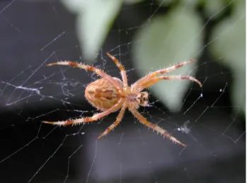
Pajekis a program, for Windows, for analysis and visu-alization oflarge networkshaving some thousands or even millions of vertices. In Slovenian language the word pa-jek means spider. The latest version of Pajek is freely available, for noncommercial use, at its home page: http://vlado.fmf.uni-lj.si/pub/networks/pajek/
We started the development of Pajek in November 1996. Pajek is im-plemented in Delphi (Pascal). Some procedures were contributed by Matjaˇz Za-verˇsnik.
The main motivation for development of Pajek was the observation that there exist several sources of large networks that are already in machine-readable form. Pajek should provide tools for analysis and visualization of such net-works: collaboration networks, organic molecule in chemistry, protein-receptor interaction networks, genealogies, Internet networks, citation networks, diffusion (AIDS, news, innovations) networks, data-mining (2-mode networks), etc. See also collection of large networks at:
http://vlado.fmf.uni-lj.si/pub/networks/data/
The design of Pajekis based on our previous experiences gained in devel-opment of graph data structure and algorithms libraries Graph and X-graph, col-lection of network analysis and visualization programs STRAN, RelCalc, Draw, Energ, and SGML-based graph description markup language NetML.
http://vlado.fmf.uni-lj.si/pub/networks/default.htm
cut-out reduction local global hierarchy context inter-links
Figure 2: Approaches to deal with large networks The main goals in the design ofPajekare:
• to support abstraction by (recursive)decompositionof a large network into several smaller networks that can be treated further using more sophisticated methods;
• to provide the user with some powerfulvisualizationtools;
• to implement a selection ofefficient (subquadratic)algorithmsfor analysis of large networks.
With Pajekwe can: find clusters (components, neighbourhoods of ‘impor-tant’ vertices, cores, etc.) in a network, extract vertices that belong to the same clusters andshowthem separately, possibly with the parts of the context (detailed local view),shrinkvertices in clusters and show relations among clusters (global view).
Besides ordinary (directed, undirected, mixed) networksPajeksupports also multi-relational networks,2-mode networks(bipartite (valued) graphs – networks between two disjoint sets of vertices), andtemporal networks(dynamic graphs – networks changing over time).
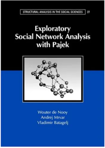
Figure 3: Pajektextbook
This manual provides short explanations of all procedures implemented in the last version ofPajek. The novice users we advise to read thePajektextbook [31]
de Nooy W., Mrvar A., Batagelj V. (2002) Exploratory Social Net-work Analysis With Pajek. Structural Analysis in the Social Sci-ences 27, Cambridge University Press, 2005.
For an overview ofnetwork analysis withPajeksee the NICTA workshop slides [5].
2
Data objects
InPajeksix types of objects are used:
Figure 4: Pajek’s Main Window
1. Networks – main objects (vertices and lines). Default extension: .net.
Network can be presented on input file in different ways: • using arcs/edges (e.g. 1 2 – line from 1 to 2)
• using arcslists/edgeslists (e.g. 1 2 3 – line from 1 to 2 and from 1 to 3) • matrix format
• UCINET, GEDCOM, chemical formats. . .
Additional information for network drawing can be included in input file as well. This is explained in the sectionExports to EPS/SVG/VRML.
2. Partitions– they tell for each vertex to which class vertex belong. Default extension: .clu.
3. Permutations– reordering of vertices. Default extension: .per.
4. Clusters– subset of vertices (e.g. one class from partition). Default exten-sion:.cls.
5. Hierarchies– hierarchically ordered vertices. Example:
Root
g1 g2
g11 g12 v5,v6,v7
Root has two subgroups – g1 and g2. g2 is a leaf – cluster with vertices v5,v6 and v7. g1 has two subgroups – g11 and g12. . . Default extension:
.hie.
6. Vectors– they tell for each vertex some numerical property (real number). Default extension:.vec.
By double clicking on selected network, partition,... you can show the object on screen.
The procedures inPajek’s main window (see Figure4) are organized accord-ing to the types of data objects they use as input.
Permutations, partitions and vectors can be used to store properties of vertices measured in different scales: ordered, nominal (categorical) and numeric.
3
Main Window Tools
3.1
File
Input/Output manipulation with the six data objects. • Network – N
– Read– Read network from Ascii file.
– Edit– Edit network. Choose vertex, show its neighbors and then: ∗ add new lines to/from selected vertex (by left mouse double
click-ing on Newline);
∗ delete lines (by left mouse double clicking);
∗ change value of line (by single right mouse clicking);
∗ subdivide line to two orthogonal lines using new invisible vertex (by single middle mouse clicking).
– Save– Save selected network to Ascii file.
If network represents Ore graph with the following five relations (arcs): 1. Wi→Hu, 2. Mo→Da, 3. Mo→So, 4. Fa→Da, 5. Fa→So
it can be stored as GEDCOM file.
The other possibility is Pajek Ore graph: 1.Fa→Ch, 2.Mo→Ch, 3.Hu-Wi (edge), or 1.Pa→Ch, 3.Hu-3.Hu-Wi (edge).
– Export Matrix to EPS– write matrix in EPS format:
∗ Original– using default numbering (for 1-mode and 2-mode net-works).
∗ Using Permutation – using current permutation. Additionally lines can be drawn to divide different classes defined by selected partition. Option can be used for 1-mode and 2-mode networks. ∗ Using Partition – using current partition. In the text window
number and density of lines among classes (and vertices in se-lected two classes) are displayed. Additionally matrix is exported to EPS where density is expressed using shadowing:
1. Structural – Densities are normalized according to maxi-mum possible number of lines among classes (suitable for dense networks).
2. Delta– Densities are normalized according to vertices having the highest number of input andoutput neighbors in classes (suitable for sparse networks).
∗ Diamonds for Negative Values, Circles for 0– Squares are used for posititive values, diamonds for negative and circles for value 0 (useful for black and white printing).
∗ Diamonds, Circles and Lines in GreyScale– Diamonds, circles and dividing lines are drawn in greyscale (not in red, green and blue).
∗ Labels on Top/Right – Labels are written on the top and on the right of the matrix - suitable for longer labels.
∗ Only Black Borders– All squares in matrix have black borders, otherwise dark squares will have white and light squares will have black borders.
∗ Thick Boundary Line– Use thicker line for dividing clusters. ∗ Large Squares/Diamonds/Circles– Use larger or smaller squares,
diamonds, and circles.
∗ Use Partition Colors for Vertex Labels – Labels of vertices are displayed using partition colors.
– Change Labelof selected network.
– Disposeselected network from memory. • Time Events Network – N
– Read Time Events– Read time network described using time events. See Table1.
List of properties s can be empty as well. If several edges (arcs) can connect two vertices, additional tag like:k(k-th line) must be given to determine to which line the command applies. E.g. command HE:3 14 37results in hiding the third edge connecting vertices14and37. Example of time network described using time events:
*Vertices 3 *Events TI 1 AV 2 "b" TE 3 HV 2 TI 4 AV 3 "e" TI 5 AV 1 "a" TI 6 AE 1 3 1 TI 7 SV 2 AE 1 2 1
Table 1: List of time events.
Event Explanation
TIt initial events – following events happen when
time pointtstarts
TEt end events – following events happen when
time pointtis finished
AVvns add vertexvwith labelnand propertiess
HVv hide vertexv
SVv show vertexv
DVv delete vertexv
AAuvs add arc(u,v)with propertiess
HAuv hide arc(u,v)
SAuv show arc(u,v)
DAuv delete arc(u,v)
AEuvs add edge(u:v)with propertiess
HEuv hide edge(u:v)
SEuv show edge(u:v)
DEuv delete edge(u:v)
CVvs change vertex property – change property of vertexvtos
CAuvs change arc property – change property of arc(u,v)tos
CEuvs change edge property – change property of edge(u:v)tos
CTuv change type – change (un)directedness of line(u,v)
CDuv change direction of arc(u,v)
PEuvs replace pair of arcs(u,v)and(v,u)by single edge(u:v)
with propertiess
APuvs add pair of arcs(u,v)and(v,u)
with propertiess
DPuv delete pair of arcs(u,v)and(v,u)
EPuvs replace edge(u:v)by pair of arcs(u,v)and(v,u)
TE 7 DE 1 2 DV 2 TE 8 DE 1 3 TE 10 HV 1 TI 12 SV 1 TE 14 DV 1
See also other possibility: description of time network using time in-tervals.
– Save– Save time network in time events format. • Partition – C
– Readpartition from Ascii file.
– Editpartition (put vertices to classes).
– Saveselected partition to Ascii file.
– Change Labelof selected partition.
– Disposeselected partition from memory. • Permutation – P
– Readpermutation from Ascii file.
– Editpermutation (interchange positions of two vertices).
– Saveselected permutation to Ascii file.
– Change Labelof selected permutation.
– Disposeselected permutation from memory. • Cluster – S(list of selected vertices)
– Readcluster from Ascii file.
– Editcluster (add and delete vertices).
– Saveselected cluster to Ascii file.
– Change Labelof selected cluster.
– Disposeselected cluster from memory. • Hierarchy – H
– Edit hierarchy (change types and names of nodes, or show vertices (and subtree) belonging to selected node). Nodes can be pushed up and down within hierarcy.
– Saveselected hierarchy to Ascii file.
– Change Labelof selected hierarchy.
– Disposeselected hierarchy from memory. • Vector – V
– Readvector from Ascii file.
– Editvector (change components of vector).
– Saveselected vector(s) to Ascii file. If cluster representing vector id’s is present, all vectors with corresponding id numbers will be saved to the same output file. Vector’s id can be added to cluster by pressing V on the selected vector (empty cluster should be created first). All vectors must have the same dimensions.
– Change Labelof selected vector.
– Disposeselected vector from memory. • PajekProject File – *.paj
– ReadPajekproject file (file containing all possiblePajekdata ob-jects – networks, partitions, permutations, clusters, hierarchies and vectors).
– Saveall currently loaded objects as aPajekproject file.
• Repeat session– During program execution all commands are written to file*.log. In this way you can repeat any execution by running selected
log file. If you change in the log file a name of a file to ?, program will ask for name when running logfile next time (so you can repeat the same sequence of steps – logfile with different input data). If startup logfile (Pa-jek.log) exists (in the same directory as Pajek.exe), it is automatically exe-cuted every time whenPajekis run.
• Show Report Window– Bring the report window in the front in the case that it was closed or is not visible.
3.2
Net
Operations, for which only a network is needed as input. • Transform
– Transpose– Transposed network of selected network: ∗ 1-Mode- Change direction of arrows.
∗ 2-Mode- Interchange Rows and Cols.
– Remove
∗ Selected Vertices– Remove selected vertices from network. ∗ all Edges– Remove all edges from selected network.
∗ all Arcs– Remove all arcs from selected network.
∗ Multiple Lines – Remove all multiple lines from selected net-work.
1. Sum Values – Values of all deleted lines are added to not deleted line between corresponding two vertices.
2. Number of Lines– Value of line between two vertices in a new network correspond to the number of lines between the two vertices in original network.
3. Min Value– Minimum value of all lines between two vertices is selected.
4. Max Value– Maximum value of all lines between two ver-tices is selected.
5. Single Line – Value of line between two vertices in a new network is 1.
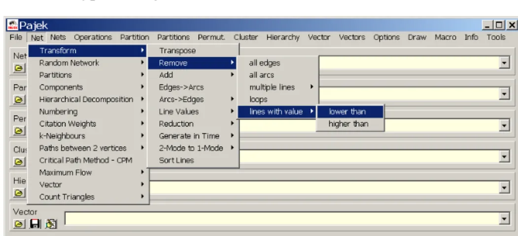
∗ Loops– Remove all loops from selected network. ∗ Lines with Value
1. lower than– Remove all lines with value lower than specified value.
2. higher than– Remove all lines with value higher than speci-fied value.
3. within interval– Remove all lines with values within speci-fied interval.
∗ all Arcs from each Vertex except
1. k with Lowest Line Values – Sort lines around vertices in ascending order according to output line values. Keep only selected number of lines with lowest values.
2. k with Highest Line Values – Sort lines around vertices in descending order according to output line values. Keep only selected number of lines with highest values.
3. keep Lines with Value equal to the k-th Value– Determine what to do with lines with value equal to the k-th value (re-move them or not).
∗ Triangle– Remove arcs belonging to lower or upper triangle.
– Addadditional vertices, lines or vertices/lines labels to network. ∗ Vertices– Copy network to new network. Dimension can be
en-larged for selected number of vertices (additional vertices without lines are added).
∗ Source and Sink– If network is acyclic, add unique first and last vertex (new network has two artificial vertices).
∗ Default Vertex Labels – Replace current labels of vertices by default vertices labels (v1, v2...).
∗ Vertex Labels from File– Replace the default vertices labels (v1, v2...) by labels given in a file.
∗ Line Labels as Line Values – replace labels of lines (or create new if there are no) with line values. Number of decimal places is the same as used in Draw window for marking lines with line values.
∗ Sibling edges– Add sibling edges to vertices with a common 1. Input– arc-ancestor
2. Output– arc-descendant
– Edges→Arcs– Convert all edges to arcs (in both directions) (make directed network).
– Arcs→Edges
∗ All– Convert all arcs to edges (make undirected network). ∗ Bidirected only– Convert only arcs in both directions to edges:
1. Sum Values– Value of the new edge is the sum of values of both arcs.
2. Min Value– Value of the new edge is the smaller of values of arcs.
3. Max Value– Value of the new edge is the larger of values of arcs.
∗ Select Min Value – If there exist bidirected arcs between two vertices retain only the arc with lower value and remove the arc with higher value. If both values are equal replace both arcs with an edge.
∗ Select Max Value – If there exist bidirected arcs between two vertices retain only the arc with higher value and remove the arc with lower value. If both values are equal replace both arcs with an edge.
– Line Values– Transformations of line values:
∗ Recode– Display frequency distribution of line values according to selected intervals and recode line values in this way.
∗ Multiply bya constant. ∗ Add Constantto line values.
∗ Constant– min or max of line value and selected constant. ∗ Absoluteline values.
∗ Absolute + Sqrt– square root of line values. ∗ Truncate– truncated line values.
∗ Exp– exponent of line values. ∗ Ln– natural logarithm of line values. ∗ Power– selected power of line values. ∗ Normalize
1. Sum– normalize so that the sum of line values will be 1 2. Max– normalize so that the maximum line value will be 1
– Reduction
∗ Degree – (Recursively) delete from network all vertices with de-gree lower than selected value (according to Input, Output or All degree). Operation can be limited to selected cluster.
∗ Hierarchical – Recursively delete from network all vertices that have only 0 or 1 neighbor. Results: simpler network and hierarchy with deleted vertices. Original network can be later restored (if we forget directions of lines).
∗ Subdivisions– Recursively delete from network all vertices that have exactly 2 neighbors (together with corresponding two lines) and (instead of that) add direct line between these two neighbors. Result is simpler network (for drawing). Original network cannot be restored!
Figure 6: Part of Reuters Terror News network on the 36th day.
∗ Design (flow graph)Reduction of all structural parts of network according to McCabe (for programs – flow graphs) [50].
– Generate in Time – Generate network in specified time(s) or interval. Input first time, last time and step (integers).
Additional parameters when vertices and lines are active should be given in network to perform this operation. They must be given be-tween signs[and]:
-is used to divide lower and upper limit of interval,
,is used to separate intervals,
*means infinity. Example: *Vertices 3 1 "a" [5-10,12-14] 2 "b" [1-3,7] 3 "e" [4-*] *Edges 1 2 1 [7]
1 3 1 [6-8]
Vertex ’a’ is active from times 5 to 10, and 12 to 14, vertex ’b’ in times 1 to 3 and in time 7, vertex ’e’ from time 4 on. Line from 1 to 2 is ac-tive only in time 7, line from 1 to 3 in times 6 to 8.
The lines and vertices in a temporal network should satisfy the consis-tency condition: if a line is active in timet then also its end-vertices are active in time t. When generating time slices of a given temporal network only ’consistent’ lines are generated.
Note that time records should always be written as last in the row where vertices / lines are defined.
See also other possibility of describing time network: description of time network usingtime events.
∗ All– Generate all networks in specified times.
∗ Only Different– Generate network in specified time only if the new network will differ in at least one vertex or line from the last network which was generated.
∗ Interval – Generate network with vertices and lines present in selected interval.
– 1-Mode to 2-Mode– Generate 2-mode network from any network.
– 2-Mode to 1-Mode – Generate an ordinary (1-mode) network from 2-mode (affiliation) network. Result is a valued network. To store a 2-mode network in input file use Pajekor Ucinet format (look at Davis.datfrom Ucinet dataset).
∗ Rows – Result is a network with relations among row elements (actors). The value of line tells number of common events of the two actors.
∗ Columns – Result is network with relations among column ele-ments (events). The value of a line tells number of actors that took part in both events.
∗ Include Loops – If checked, loops with value telling the total number of events for each actor (total number of actors for each event), are added.
∗ Multiple Lines – Generate nonvalued 1-mode network, where multiple lines among vertices can exist. The label of the gen-erated line corresponds to the label of the event/actor that served to induce the line. If partition of the same dimension is present, multirelational network can be generated.
∗ Normalize 1-Mode – Normalize the obtained 1-Mode network. 1-Mode network must be obtained with optioninclude loops check-ed, andmultiple linesnot checked:
Geoij = aij √ aiiajj Inputij = aij ajj Outputij = aij aii Minij = aij min(aii, ajj) Maxij = aij max(aii, ajj) MinDirij = aij aii aii≤ajj 0 otherwise MaxDirij = aij ajj aii≤ajj 0 otherwise
The obtained network is usually not sparse. To make it sparser
useNet/Transform/Remove/lines with value/lower than.
∗ Rows=Cols– Transform 2-Mode network with the same subsets of vertices to 1-Mode network.
∗ Cols=0– Transform 2-Mode network to 1-Mode network by set-ting number of columns to 0. The result is the same as changing for example*Vertices 32 18to*Vertices 32 in input
network file.
– Multiple Relations
∗ Extract Relation(s) – Extract one or selected list of relations from selected multiple relations network.
∗ Canonical Numbering– Enumerate relations with sequential num-bers 1, 2,. . .
∗ Generate 3-Mode Network – generate a 3-mode network from 1-mode or 2-mode multirelational network. For each line in mul-tirelational network r: i j v(line from i toj with valuev, relation number isr) generate the following three lines (triangle):
· 1-mode networks:
i 2N+r v N+j 2N+r v · 2-mode networks: i j v i N+M+r v j N+M+r v
where Nis cardinality of the first mode and M cardinality of the second mode.
∗ Line Values−>Relation Numbers– Store line values as rela-tion numbers (absolute truncated values).
∗ Relation Numbers−>Line Values– Store relation numbers as line values.
∗ Change Relation Number - Label – Change selected relation number to new relation number with corresponding label.
– Sort Lines–
∗ Neighbors around Vertices – For each vertex sort lines con-nected to it in ascending order according to other end-vertex. ∗ Line Values– Sort lines in ascending or descending order
accord-ing to line values.
• Random Network– Generate random network of selected dimension
– Total No. of Arcs – Generate random directed network of selected dimension and given number of arcs.
– Vertices Output Degree – Generate random directed network of se-lected dimension and output degree of each vertex in given range.
– Bernoulli/Poisson– Generate undirected, directed, acyclic, bipartite or 2-mode random network according to model defined by Bernoulli / Poisson: each line is selected with the given probability p. Instead of p, which is for large and sparse networks (very) small number, in Pajeka more intuitiveaverage degreedis used. They are connected with relationsd= 1
n
P
v∈V deg(v) = 2mn andm =pM wheren =|V|,
m =|L|andM is the number of lines in maximal possible network – for example, for undirected graphsM =n(n−1).
– Scale Free – Generate scale free undirected, directed or acyclic net-work. The procedure is based on a refinement of the model for gener-atingscale free networks, proposed in [55]. At each step of the growth a new vertex andk edges are added to the networkN. The endpoints
of the edges are randomly selected among all vertices according to the probability Pr(v) = αindeg(v) |E| +β outdeg(v) |E| +γ 1 |V| whereα+β+γ = 1. It is easy to check thatP
v∈V Pr(v) = 1.
– Small World – Generate Small world random network. See [12].
– Extended Model – Generate random network according to extended model defined by Albert and Barabasi [3].
• Partitions– Partitioning Network. Result is a Partition.
– Degree
∗ Input– Number of lines into vertices. ∗ Output– Number of lines out of vertices. ∗ All– Number of neighbors of vertices.
– Domain – For each vertex compute its domain according to input, outputorallneighbors. Results are:
∗ Partition containing size of domain - number of reachable ver-tices.
∗ Vector containing the normalized size of domain - normalization is done by total number of vertices – 1.
∗ Vector containing the average distance from/to domain.
Proximity Prestige index can be computed by dividing the normalized size of domain by average distance.
– Core–k-core is a subnetwork of given network where each vertex has at leastkneighbors in the same core according to:
∗ Input... lines coming into vertex. ∗ Output... lines going out of vertex. ∗ All... all neighbors.
∗ 2-Mode – core partition of a 2-mode network. Given minimum degree in first (k1) and minimum degree in second subset (k2) a new partition is generated where 0means that vertex does not belong to the core of prespecifiedk1 andk2,1means that vertex belongs to that core.
2682562 3322485 3636168 3666948 3691755 3697150 3767289 3773747 3796479 3795436 3876286 3891307 3947375 3954653 3960752 3975286 4011173 4000084 4013582 4029595 4017416 4032470 4077260 4082428 4083797 4113647 4130502 4118335 4149413 4154697 4195916 4198130 4202791 4229315 4261652 4290905 4293434 4302352 4330426 4340498 4349452 4357078 4361494 4368135 4386007 4387038 4387039 4400293 4415470 4419263 4422951 4455443 4456712 4460770 4480117 4472293 4472592 4502974 4510069 4514044 4526704 4550981 4558151 4583826 4621901 4630896 4657695 4659502 4695131 4704227 4709030 4719032 4710315 4713197 4721367 4752414 4770503 4795579 4797228 4820839 4832462 4877547 4957349 5016988 5122295 5016989 5124824 5171469 5283677 5555116
∗ 2-Mode Review– Given starting values ofk1 andk2 the follow-ing list is computed:
k1 k2Rows Cols Comp
where k1 is minimum degree in the first, k2 minimum degree in the second subset,RowsandColsare number of vertices in first and second subset respectivelly andComp, number of connected components in network induced by k1 andk2. k1 andk2 are in-cremented until the resulting network is empty.
∗ 2-Mode Border– Compute only border values ofk1andk2for a given 2-mode network.
– Valued Core – Generalizedk-core: Instead of counting lines (neigh-bors) use values of lines. sum of lines or maximum value can be used when computing valued core:
Sum valued core of threshold val is a subnetwork of given network where the sum of values of lines to (from) the members of the same core is at leastval.
Max valued core of threshold val is a subnetwork of given network where the maximum value of all lines to (from) the members of the same core is at leastval.
Threshold values must be given in advance. Two different ways to determine thresholds:
∗ First Threshold and Step– Select first threshold value and step in which to increase threshold.
∗ Selected Thresholds– Thresholds (increasing numbers) are given using vector.
∗ 2-Mode– valued core (according to line values) partition of a 2-mode network. Given minimum valued degree in first (k1) and minimum valued degree in second subset (k2) a new partition is generated where0means that vertex does not belong to the valued core of prespecifiedk1andk2,1means that vertex belongs to that core.
Additionally (for 1-mode networks), Input, Output or All valued cores can be used.
– Depth
∗ Acyclic – Partition acyclic network according to depths of ver-tices.
∗ Genealogical – Partition network that represents genealogy ac-cording to layers of vertices.
∗ Generational – Partition network that represents genealogy ac-cording to layers of vertices. The same as genealogical partition but with less layers.
– p-CliquesPartition network according top-Cliques (partition to clus-ters where vertices have at least proportionp(number between 0 and 1) neighbors inside the cluster.
∗ Strong... for directed network. ∗ Weak... for undirected network.
– Vertex Labels– Partition vertices with same labels to the same class numbers (for molecule).
– Vertex Shapes– Partition vertices with same shapes (ellipse, box, dia-mond) to the same class numbers (used in genealogy to show gender).
– Islands– Partition vertices of network with values on lines (weights) to cohesive clusters (weights inside clusters must be larger than weights to neighborhood): the height of vertex (vector) is defined as the maxi-mum weight of the neighbor lines. Two options:
∗ Line Weights
∗ Line Weights [Simple]
New network with only lines constituting islands can be generated if
Generate Network with Islandsis checked.
– Bow-Tie – Partition vertices of directed network (graph structure of the web) to the following classes: 1 – LSCC, 2 – IN, 3 – OUT, 4 – TUBES, 5 – TENDRILS, 0 – OTHERS.
– 2-Mode– Partition of vertices of a 2-mode network into two subsets.
– Default Labels Partition – Input is network with default vertex la-bels: e.g., v3,v9,... Result is a partition of selected dimension, where vertices defined by numbers stored in vertex labels (e.g., 3, 9,...) go to cluster 1, other vertices go to cluster 0.
Operation can be used to make other objects (e.g. partitions, vectors, ...) compatible with a network, if network is reduced by several oper-ations (e.g. extractions).
• Components
– Strong– Strong Components of selected network.
– Strong-Periodic– Strong Periodic Components of selected network -strongly connected components are further divided according to peri-ods.
Figure 8: Bow-tie – Graph structure in the web [26]
– Weak– Weak Components of selected network.
– Bi-Components– Biconnected Components of selected network. Ar-ticulation points belong to several classes, so the result cannot be stored in partition – biconnected components are stored in hierarchy! Minimal number of vertices in components can be selected. Addition-ally, partition containing articulation points is produced: number of biconnected components to which each vertex belongs is given. Par-tition containing vertices belonging to exactly one bicomponent, ver-tices outside bicomponents and articulation points is also produced: vertices outside bicomponents get class zero, each bicomponent is numbered consecutively (from 1 to number of bicomponents) and ar-ticulation points get class number 9999998.
• Hierarchical Decomposition
– Clustering* – Hierarchical clustering procedure. Input is dissimilar-ity network (matrix), which can be obtained using
Operations/Dissimilarity/Network basedor read from input file. ∗ Run– Hierarchical clustering procedure. Result is hierarchy with
∗ Options – Select method for hierarchical clustering procedure (general, minimum, maximum, average, ward, squared ward).
– Symmetric-Acyclic – Symmetric-Acyclic decomposition of network. Result is hierarchy with nested clusters [33].
– Clustering with Relational Constraint– Hierarchical clustering with relational constraint procedure. See:
Ferligoj A., Batagelj V. (1983): Some types of clustering with rela-tional constraints. Psychometrika,48(4), 541-552.
Only dissimilarities among vertices that are linked are taken into ac-count what enables to find clusterings very fast also for large networks. Input is network with dissimilarities, which can be obtained using Operations/Dissimilarity/Network orVector basedor read from input file.
∗ Run– Results are: a partition representing tree: fathers of nodes; and two vectors: describing heights of nodes and number of ver-tices in subtree respectivelly. If network has n vertices then ob-tained partitions and vectors have dimension 2*n-1. Note that this objects are not compatible with original network, you must useMake Partitionto get compatible results.
∗ Make Partition– From obtained partition representing tree gen-erate partition compatible with original network
· using Threshold determined by Vector – From obtained partition representing tree and one of the two vectors (all have dimension 2*n-1) generate partition compatible with original network by giving threshold value.
· with selected Size of Clusters– From obtained partition rep-resenting tree and given number of vertices in clusters gener-ate partition compatible with original network.
∗ Extract Subtree as Hierarchy – Extract subtree from obtained Partition by giving the root as Pajek Hierarchy.
∗ Options – Select method for hierarchical clustering with rela-tional constraint (minimum, maximum, or average) and strategy (strict,leader, ortolerant).
• Numbering
– Depth First– Depth first numbering of selected network... ∗ Strong... taking directions of arcs into account. ∗ Weak... forget directions (or undirected network).
– Breadth First– Breadth first numbering of selected network... ∗ Strong... taking directions of arcs into account.
∗ Weak... forget directions (or undirected network).
– Reverse Cuthill-McKee– RCM numbering.See paper.
– Core + Degree– Numbering in decreasing order according to all core partition. Within the same core number vertices are ordered in de-creasing order according to number of neighbors which have the same or higher core number.
• Citation Weights – If a network represents citation network, weights of lines (citations) and vertices (articles) can be computed. Results are:
– Network with values on lines representing importance of citations.
– Binary partition with vertices on the main path.
– Network containing only main path.
– Vector with importance of vertices (articles). Different methods of assigning weights [43]:
– Search Path Count (SPC)– method. Compute from Source to Sink.
– Search Path Link Count (SPLC) – method. Each vertex is consid-ered as Source.
– Search Path Node Pair (SPNP)– method.
Weights can also be normalized (using flow or maximum value) or logged. • k-neighbors– Select all vertices
– Input...from which we can reach selected vertex in at mostk-steps.
– Output...that can be reached from selected vertex in at mostk-steps.
– All...Input + Output (forget direction of lines)
Result is partition where vertices are in class numbers equal to the dis-tance from given vertex, vertices that cannot be reached from selected vertex are in class number 9999998. After you have a partition you can extract subnetwork.
– From Clusters– Compute selected distances according to each vertex in Cluster. Results consist of so many partitions as is the number of vertices in cluster. Instead of storing results in partitions they can be stored in vectors as well.
• Paths between 2 vertices
– One Shortest – Find the shortest path between two vertices. Result is new network. Values on lines can be taken into account (if they present distances between vertices) or not (graph theoretical distance). The latter possibility is faster.
– All Shortest – Find all shortest paths between two vertices. Result is new network. Values on lines can be taken into account (if they present distances between vertices) or not (graph theoretical distance). The latter possibility is faster.
– Walks with Limited Length– Find all walks between two vertices with limited maximum length.
– Diameter– Find diameter – the length of the longest shortest path in network and corresponding two vertices. Full search is performed, so the operation may be slow for very large networks (number of vertices larger than 2000).
– Geodesics Matrices* – Compute the shortest path length matrix and the geodesics count matrix (for small networks only!).
– Distribution of Distances – Compute distribution of lengths of the shortest paths and average path length among all reachable pairs of vertices in network.
∗ From All Vertices– Take all vertices as starting points.
∗ From Vertices in Cluster– Only distances from vertices selected by Cluster are computed.
• Critical Path Method (CPM)– Find the critical path in acyclic network – result is new network containing the critical path. Algorithm can be used in the area of project planning but also for analysing acyclic graphs. Addi-tional networks containing total and free delay times of activities are gener-ated. Two vectors (partitions) are generated, too: First containing the earli-est possible times of coming into given states and the second containing the latest feasible times of coming into given states.
• Maximum Flowamong vertices.
– Selected Pair – Find maximum flow between selected two vertices (algorithm looks for paths to be saturated and among them it always selects the shortest path). Algorithm can be used in the technical area (actual flow, values on lines mean capacities) or for analysing graphs (if all values are 1). Result is a new network, containing the two ver-tices and lines contributing to maximum flow between them.
– Pairs in Cluster– Find maximum flow among vertices determined by cluster. Result is a new network, where a value on line means max-imum flow between corresponding two vertices. Algorithm is slow: Use it on smaller networks or clusters with limited number of vertices only!
• Vector– Get vector from network
– Centrality – Result is a vector containing selected centrality measure of each vertex and centralisation index of the whole network [64, p. 169-219].
∗ Closenesscentrality (Sabidussi).
1. Input – centrality of each vertex according to distances of other vertices to selected vertex.
2. Output– centrality of each vertex according to distances of selected vertex to all other vertices.
3. All – forget direction of lines – consider network as undi-rected.
∗ Betweennesscentrality (Freeman).
– Get Loops – store values of loops to vector.
– Get Coordinate – x, y, or z coordinate of network. You can also get all coordinates at once - possibility to have more than 3 coordinates, coordinates must contain character . (dot).
– Important Vertices – Find important vertices in directed network (e.g. web pages, scientific citations) or 2-mode network. Result are vectors with weights and partition with selected number of important vertices.
∗ 1-Mode: Hubs-Authorities – In directed networks we can usu-ally identify two types of important vertices:hubsandauthorities [47]. A vertex is a good hub, if it points to many good authorities, and it is a good authority, if it is pointed to by many good hubs. In obtained partition value 1 means, that the vertex is a good author-ity, value 2 means, that the vertex is a good authority and a good hub, and value 3 means, that the vertex is a good hub.
∗ 2-Mode: Important Vertices – Generalization of algorithm for 2-mode networks – find important vertices from first and second subset.
– Structural Holes– Burt’s measure of constraint (structural holes) [27, page 54-55]. Results are:
∗ network pij: the proportion of the value of i’s relation(s) withj compared to the total value of all relations of i. whereaij is the value of the line fromitoj
pij =
aij +aji
P
k(aik+aki)
∗ network containing dyadic constraintcij– the constraint of absent primary holes around j on i: Explanation: Contact j constrains youri’s entrepreneurial opportunities to the extent that:
(a) you’ve made a large investment of time and energy to reachj, and
(b)j is surrounded by few structural holes with which you could negotiate to get a favorable return on the investment.
cij = (pij +
X
k,k6=i,k6=j
pikpkj)2
∗ vector containing aggregate constraintCi: Ci =Pjcij,
Ci = 1for isolated vertices.
– Clustering Coefficients– Compute different inherent tendency coef-ficients in undirected network:
Let deg(v) denotes degree of vertex v, |E(G1(v))| number of lines among vertices in 1-neighborhood of vertex v, MaxDeg maximum degree of vertex in a network, and|E(G2(v))|, number of lines among vertices in1and2-neighborhood of vertexv.
∗ CC1– coefficients considering only1-neighborhood:
CC1(v) = 2|E(G1(v))| deg(v)·(deg(v)−1) CC 0 1(v) = deg(v) MaxDegCC1(v)
∗ CC2– coefficients considering 2-neighborhood
CC2(v) =
|E(G1(v))| |E(G2(v))|
CC20(v) = deg(v)
MaxDegCC2(v)
Ifdeg(v)≤1all coefficients for vertexvget missing value (9999998). Watts-Strogatz Clustering Coefficient (Transitivity) and Network Clus-tering Coefficient are also reported.
– Summing up Values of Lines– Sum values of all incoming, outgoing or all lines connected to selected vertex.
– Min of Values of Lines– Find minimum value of incoming, outgoing or all lines connected to selected vertex.
– Max of Values of Lines– Find maximum value of incoming, outgoing or all lines connected to selected vertex.
– Centers– Find centers in a graph using ’robbery’ algorithm: vertices that have higher degrees (are stronger) than their neighbors steal from them:
∗ at the beginning give to vertices initial strength according to their degrees, or start with value 1
∗ when ’weak’ vertex is found, neighbors steal from it according to their strengths, or they steal the same amount
– PCore– generalized cores. ∗ Degree– ordinary cores.
∗ Sum– taking values of lines into account (sum of values of lines inside pcore).
∗ Max– taking values of lines into account (max of values of lines inside pcore).
• Count- how many times each line belongs to predefined rings
– 3-Rings – For each line count number of 3-rings to which the line belongs.
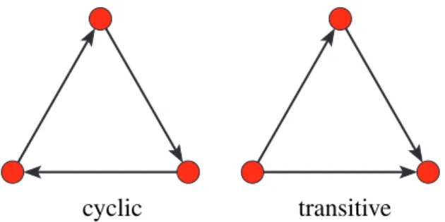
∗ Undirected– for undirected networks – count undirected 3-rings. ∗ Directed– for directed networks – countcyclic,transitive, or all 3-rings, or count how many times each line is a transitive shortcut (see Figure9).
– 4-Rings – For each line count number of 4-rings to which the line belongs.
∗ Undirected– for undirected networks – count undirected 4-rings. ∗ Directed– for directed networks – countcyclic,diamonds,gen
ea-logical, transitive, or all 4-rings, or count how many times each line is a transitive shortcut (see Figure10).
3.3
Nets
cyclic transitive
Figure 9: Lines belonging to cyclic and transitive (shortcut) 3-rings
cyclic transitive genealogical diamond Figure 10: Types of directed 4-rings on arcs
• Union of lines – Fuse selected networks. Result is a multiple relations network. If you want to get union of networks, multiple lines must still be deleted. Networks must match in dimension or: If one network hasm
vertices and othernvertices andm < nthen in network withnvertices first
mvertices must match with vertices in network withmvertices.
• Cross-Intersection – Intersection of selected networks. Networks must match in dimension or: If one network has m vertices and other n ver-tices andm < nthen in network withnvertices firstmvertices must match with vertices in network withmvertices. Values of lines in intercept can be sum, difference, product, quotient, min, or maxof both values.
• Intersection– Intersection of selected networks where relation numbers are taken into account.
• Cross-Difference– Difference of selected networks.
• Difference – Difference of selected networks where relation numbers are taken into account.
• Fragment (1 in 2)– Find all instances of fragment (determined by network 1) in network 2.
– Find– Execute command.
– OptionsSelect appropriate model of fragment.
∗ Induced – there should be no additional lines between vertices in instance of fragment to match (stronger condition) otherwise additional lines can be present (weaker).
∗ Labeled– labels must match (e.g. atoms in molecule). Labels are determined by classes (colors) in partition - first partition and sec-ond partition must be selected before searching for labeled frag-ments. First partition determines ’labels’ of first network (frag-ment), second partition determines ’labels’ of second (original) network.
∗ Check values of lines – values of lines must match (e.g. in ge-nealogy values represent sex: 1 – man, 2 – woman).
∗ Check relation number– relation numbers must match.
∗ Check only cluster – only fragments are searched. where first vertex is one of the vertices in cluster.
∗ Extract subnetwork– produce additional result: extract subnet-work containing vertices belonging to fragments and correspond-ing lines.
· Retain all vertices after extracting – in extracted network the same vertices as in original network are present, only lines which do not belong to any fragment are removed.
∗ Same vertices determine one fragment at most – how frag-ments on the same set of vertices are treated: if not checked – fragments with the same set of vertices are allowed.
· Create Hierarchy with fragments– result of fragment search-ing is also a Hierarchy with vertices in fragments (available only if Same vertices determine one fragment at most is not checked.
∗ Repeating vertices in fragment allowed– same vertices can ap-pear in fragment more than once (e.g. in cycles).
if not checked: found fragments always have the same number of vertices as original fragment
if checked: some of found fragments can have less vertices than original fragment
Damianus/Georgio/ Legnussa/Babalio/ Marin/Gondola/ Magdalena/Grede/ Nicolinus/Gondola/ Franussa/Bona/ Marinus/Bona/ Phylippa/Mence/ Sarachin/Bona/ Nicoletta/Gondola/ Marinus/Zrieva/ Maria/Ragnina/ Lorenzo/Ragnina/ Slavussa/Mence/ Junius/Zrieva/ Margarita/Bona/ Junius/Georgio/ Anucla/Zrieva/ Michael/Zrieva/ Francischa/Georgio/ Nicola/Ragnina/ Nicoleta/Zrieva/
Figure 11: Fragments – Marriages among relatives in Ragusa
• Multiply First * Second - multiply selected 1 or 2 mode networks (that match criteria for multiplication).
• Shrink coordinates (1 to 2) - Useful if you shrink network, draw shrunk network separately, and then apply all coordinates to vertices in original network (vertices in same class get the same coordinates). Replace coordi-nates in network 2 using coordicoordi-nates of shrunk network 1. Shrinking can be determined using
– Partitionor
– Hierarchy
3.4
Operations
One network and something else is needed as input.
• Shrink Network- Before starting shrinking, select appropriate blockmodel in Options menu. Default is just number of lines between shrunk vertices that must be present in original network, to cause a line in a new network.
– Partition– Shrink network according to selected partition. Vertices in class 0 are (by default) left unchanged, others are shrunk. Results are shrunken network and shrunken partition.
– Hierarchy – Shrink network according to selected hierarchy. Nodes in hierarchy that are Closed are shrunk to new vertex. Cutnodes are shrunk to virtual vertex. Bordernodes are not shrunk, but they are not visible. Vertices belonging to other nodes are left unchanged. Type of shrinking (blockmodel) can be selected in Options menu.
• Extract from Network
– Partition – Extract sub-network according to selected partition (ex-tract range of classes from partition). Ex(ex-tracted partition is produced as additional result.
– Cluster– Extract sub-network according to selected cluster.
– 2-Mode Network – Extract 2-mode network from 1-mode network: first and second mode are determined by given set of clusters in parti-tion.
– to GEDCOM – Extract sub-genealogy according to selected parti-tion (weakly connected component) to new GEDCOM file (genealogy must be read as Ore graph).
• Brokerage Roles - For each vertex j count five brokerage roles (coordi-nator, itinerant broker, representative, gatekeeperandliaison) according to given partition. j i k coordinator j i k itinerant broker j i k liaison j i k gatekeeper j i k representative • Dissimilarity*
– Network based– Compute selected dissimilarity matrix (d1,d2,d3 or
d4) among vertices in cluster according to number of common neigh-bors. Corrected Euclidean-liked5 andManhattan-liked6 dissimilari-ties can be computed as well [13]. The obtained matrix can be used further for hierarchical clustering procedure.
You can include vertex vto its own neighborhood or not and display in report window only upper triangle / undirected or complete matrix /directed (if number of vertices is low).
Nv is a set of input, output or all neighbors of vertex v; +stands for symmetric sum,∪stands for set union and\stands for set difference; |stands for set cardinality;1st maxdegreeand2nd maxdegreeare the largest degree and the second largest degree in network, respectively.
d1(u, v) = |Nu+Nv| 1st maxdegree + 2nd maxdegree d2(u, v) = |Nu+Nv| |Nu∪Nv| d3(u, v) = |Nu+Nv| |Nu|+|Nv| d4(u, v) = max(|Nu\Nv|,|Nv\Nu|) max(|Nu|,|Nv|) d5(u, v) = v u u u t n X s=1 s6=u,v ((qus−qvs)2+ (qsu−qsv)2) +p·((quu−qvv)2+ (quv−qvu)2) d6(u, v) = n X s=1 s6=u,v (|qus−qvs|+|qsu−qsv|) +p·(|quu−qvv|+|quv−qvu|) Dissimilaritiesd5 andd6 are based on some matrixQ = [quv]on ver-tices – for example on adjacency matrix or on distance matrix. The parameter pis usually set to value1or2. In the case Nu = Nv = 0 we set all dissimilaritiesd1 -d4 to1.
IfAmong all linked Vertices onlyis checked dissimilarities are com-puted as line values of given network.
– Vector based–Euclidean, Manhattan, Canberra, or (1-Cosine)/2
dissimilarities among Vectors determined by Cluster are computed as line values of given network.
• Vector– Operations on network and vector.
– Network * Vector – Ordinary multiplication of matrix (network) by vector. Result is a new vector.
– Vector # Network– Result is a new network:
∗ Input– Multiplying incoming arcs in network by corresponding vector values - multiplyingi-th column of matrix byi-th compo-nent of vector.
∗ Output– Multiplying outgoing arcs in network by corresponding vector values - multiplyingi-th row of matrix byi-th component of vector.
– Harmonic Function– See Bollobas [25, page 328].
Let(G, a)be a connected weighted graph, with weight functiona(x, y), and let S is subset of vertices V(G). A function f : V(G) → IR is said to be harmonic on(G, a), with boundaryS, if
f(x) = 1 A(x) X y (a(x, y)f(y)), ∀x∈V(G)\S A(x) =X y a(x, y) Implementation inPajek:
∗ functionf is determined by vector
∗ weight functiona(x, y)is given by (valued) network
∗ subset S is determined by partition – vertices in class 1 are in subsetS (fixed vertices), other vertices are inV(G)\S
∗ additionally, permutation determines the order of vertices in com-putations.
InPajekyou can compute the harmonic function once or iterativelly - as long as difference between successive functions become small enough. Components of vector that represents functionfcan be mod-ified immediately when they are computed or only at the end of each iteration (after all components are computed). Procedure can be run according to:
∗ Input– neighbors ∗ Output– neighbors ∗ All– neighbors
– Summing up neighbors – For each vertex compute the sum of class numbers of its neighbors according to
∗ Input– neighbors ∗ Output– neighbors ∗ All– neighbors
– Min of neighbors– For each vertex compute the minimum class num-ber of its neighbors according to
∗ Output– neighbors ∗ All– neighbors
– Max of neighbors – For each vertex compute the maximum class number of its neighbors according to
∗ Input– neighbors ∗ Output– neighbors ∗ All– neighbors
– Put Loops– put vector values as loops (arcs or edges) in current net-work.
– Put Coordinate– put vector as x, y, or z coordinate, or put it as polar radius or polar angle of vertices in network layout.
– Diffusion Partition– Compute diffusion partition according to thresh-olds given in vector. Vertices in selected cluster are considered to adopt in time 1.
– Islands– Partition vertices to cohesive clusters according to weights of vertices determined by a vector.
∗ Vertex Weights – Vertex island is a cluster of vertices of given network with weighted vertices where the weights of the vertices on the island are larger than the weights of the vertices in the neighborhood. The weights are also called heights.
∗ Vertex Weights [Simple] – Simple vertex island is vertex island with only one top.
• Transform – Transformations of network according to Partition, Cluster and/or Vector.
– Remove Lines– Removing lines according to partition.
∗ Inside Clusters – Remove all lines with incident vertices in the same (selected) cluster(s).
∗ Between Clusters – Remove all lines with incident vertices in different clusters.
∗ Between Two Clusters
1. Arcs– Remove all arcs pointing from first to second cluster. 2. Edges– Remove all edges between the selected two clusters. ∗ Inside Clusters with value
1. lower than Vector value – Remove all lines inside clusters (determined by a Partition) with value lower than the value specified in a Vector.
2. higher than Vector value– Remove all lines inside clusters (determined by a Partition) with value higher than the value specified in a Vector.
Dimension of a Vector must be equal to the highest cluster number in a Partition.
– Add– some elements to network
∗ Arcs from Vertex to Cluster– add arcs from selected vertex to all vertices in Cluster.
∗ Arcs from Cluster to Vertex– add arcs from all vertices in Clus-ter to selected vertex.
∗ Time Intervals determined by Partitions– change network to temporal network using two partitions: first partition determines initial time point, second determines terminal time point of each vertex.
– Direction – Convert to directed network where all arcs are pointing from
∗ Lower->Higherclass number. ∗ Higher->Lowerclass number. Lines inside classes may be deleted or not.
– Vector(s) ->Line Values– Replace line values with result of selected operation (sum, difference, multiplication, division) on vector(s) val-ues in corresponding terminal and initial vertices.
• Reorder
– Network – Reorder vertices in network according to selected permu-tation.
– Partition– Reorder vertices in partition according to selected permu-tation.
– Vector– Reorder vertices in vector according to selected permutation. • Count neighbor Colors– For selected network and partition a new parti-tion is generated where for each vertex the frequency of vertices of selected color in the neighborhood is given. Colors to be counted are determined using cluster.
• Coloring
– Create New– Sequential coloring of vertices in order determined by permutation. Result depends on selected permutation significantly.
– Complete Old– Complete partial coloring of vertices in order deter-mined by permutation. For example some vertices can be colored by hand, but most of the vertices are still uncolored (in class 0). In this way you can help program to produce better coloring.
• Balance* – Relocation algorithm for partitioning signed graphs (graphs with positive and negative values on lines representing friends and enemies, for example). Given partition is optimized to get as much as possible pos-itive lines inside classes and negative lines between classes. Another algo-rithm does not distinguish between diagonal and off-diagonal blocks: each block can be positive, negative, or null. If number of repetitions is higher than 1, initial partitions into given number of classes are chosen randomly for every repetition separately. If program finds several optimal solutions, all are reported. For more details about algorithm see Doreian and Mrvar [32].
Option can be used for two mode signed graphs as well: input is two mode partition. In this case algorithm tries to find as ’clear’ as possible positive, negative, and null blocks.
IfPrespecification is checked user can define a prespecified model by en-tering lettersP,N, or0to cells (to require positive, negative or null blocks) or leave cells empty (in this case the block can be of any type).
By setting penalty for small null blocks to some nonzero value, we try to get null blocks as large as possible.
• Blockmodeling*– Generalized blockmodeling of 1-mode and 2-mode net-works [7,35]. For details see Section7on page84. Descriptions of models are stored on MDL files. See also block types on page50.
– Random Start– Start the optimization with random partition(s).
– Optimize Partition– Show the criterion function for selected parti-tion and optimize it.
– Restricted Options – Show only selected part of options (sufficient for most users) or all options.
– Short Report – Show only main results of optimization in Report window (sufficient for most users) or detailed, long report.
• Genetic Structure – Compute genetic structure of given acyclic network according to given partition (of minimal vertices). As result we get as many vectors as is different clusters in partition, and the dominant gene partition. • Permutation*– Improve given permutation according to network.
World trade - alphabetic order afg alb alg arg aus aut bel bol bra brm bul bur cam can car cha chd chi col con cos cub cyp cze dah den dom ecu ege egy els eth fin fra gab gha gre gua gui hai hon hun ice ind ins ire irn irq isr ita ivo jam jap jor ken kmr kod kor kuw lao leb lib liy lux maa mat mex mla mli mon mor nau nep net nic nig nir nor nze pak pan par per phi pol por rum rwa saf sau sen sie som spa sri sud swe swi syr tai tha tog tri tun tur uga uki upv uru usa usr ven vnd vnr wge yem yug zai
afg alb alg arg aus aut bel bol bra brm bul bur cam can car cha chd chi col con cos cub cyp cze dah den dom ecu ege egy els eth fin fra gab gha gre gua gui hai hon hun ice ind ins ire irn irq isr ita ivo jam jap jor ken kmr kod kor kuw lao leb lib liy lux maa mat mex mla mli mon mor nau nep net nic nig nir nor nze pak pan par per phi pol por rum rwa saf sau sen sie som spa sri sud swe swi syr tai tha tog tri tun tur uga uki upv uru usa usr ven vnd vnr wge yem yug zai
World Trade (Snyder and Kick, 1979) - cores
uki net bel lux fra ita den jap usa can bra arg ire swi spa por wge ege pol aus hun cze yug gre bul rum usr fin swe nor irn tur irq egy leb cha ind pak aut cub mex uru nig ken saf mor sud syr isr sau kuw sri tha mla gua hon els nic cos pan col ven ecu per chi tai kor vnr phi ins nze mli sen nir ivo upv gha cam gab maa alg hai dom jam tri bol par mat alb cyp ice dah nau gui lib sie tog car chd con zai uga bur rwa som eth tun liy jor yem afg mon kod brm nep kmr lao vnd
uki net bel lux fra ita den jap usa can bra arg ire swi spa por wge ege pol aus hun cze yug gre bul rum usr fin swe nor irn tur irq egy leb cha ind pak aut cub mex uru nig ken saf mor sud syr isr sau kuw sri tha mla gua hon els nic cos pan col ven ecu per chi tai kor vnr phi ins nze mli sen nir ivo upv gha cam gab maa alg hai dom jam tri bol par mat alb cyp ice dah nau gui lib sie tog car chd con zai uga bur rwa som eth tun liy jor yem afg mon kod brm nep kmr lao vnd
Figure 12: World trade. Orderings: alphabetical and determined by clustering
– Travelling Salesman– Can be applied to dissimilarity matrix, or mod-ified matrix representing network (fill diagonal and change 0 in the matrix with some large numbers):
∗ Run – Run 3-OPT algorithm for solving Travelling Salesman Problem.
∗ Options– Put selected value on diagonal, add some artificial ver-tices, and incident lines with large values, change value 0 with selected (large) value.
– Seriaton– Starting with network and (random) permutation improve the permutation using seriation algorithm from Murtagh [53, page 11-16].
∗ 1-Mode– for ordinary (1-Mode) networks ∗ 2-Mode– for 2-Mode networks
– Clumping– Starting with network and (random) permutation improve the permutation using clumping algorithm from Murtagh [53, page 11-16].
∗ 1-Mode– for ordinary (1-Mode) networks ∗ 2-Mode– for 2-Mode networks
– R-Enumeration – Starting with network and (random) permutation find such permutation that enumeration of neighbor vertices are as close to each other as possible.
• Functional Composition – Let f be a partition or a permutation and g a partition, a permutation, or a vector. The result is new partition, permutation or vectorrdefined in the following way:r[v] = (f ∗g)[v] =g[f[v]]. • Expand Partition
– Greedy Partition– Put vertices with unknown class number (0) in the same class as selected vertices in partition if
∗ Input...we can reach selected vertices in at most k-steps.
∗ Output ...we can come to vertices from selected vertices in at most k-steps.
∗ All...Input + Output (forget direction of lines)
Classes are joined if one vertex should belong to more classes.
– Influence Partition– Put every vertex with unknown class number (0) in given partition in the same class as is the class of the closest vertex. If several vertices with known class number have the same distance, the highest value is used.
– Make Multiple Relations Network – Transform network to a mul-tiple relation network using a partition: if both endvertices of a line belong to the same class in partition the multiple relations tag will be equal to the class number of endvertices, otherwise it will be 0. • Expand Reduction– Restore original network from reduced network
(hier-archical reduction!) and appropriate hierarchy (result is always undirected network).
• Identify– Identify (reorder and/or join some units).
• Petri– Execute Petri net according to starting marking of places determined by partition. Number of places in network is equal to dimension of partition. Places must be defined first (1..m) then transitions (m+ 1..n). What to do if more than one transition can fire? Two possibilities:
– Random– Transition is chosen randomly.
– Complete– Complete tree of all possible transitions is built - result is hierarchy. You can choose the maximum depth of the tree, or execute Petri net as long as possible.
Try for examplepetri2from the book of Peterson [56, page 21] orpetri52
E1 E2 E3 E4 E5 M1
.
M2.
M3.
M4.
M5.
C1.
C2.
C3.
C4.
C5.
• Refine PartitionRefine partition according to selected network (reachabil-ity).
– Strong... for directed network.
– Weak... for undirected network.
• Leader Partition– find clusters of vertices of network inside layers.
3.5
Partition
Only Partition is needed as input.
• Create Constant Partition– Create constant partition of selected dimen-sion. Default dimension is the size of selected network (if there is one in memory).
• Create Random Partition– Create random one or two mode partition. • Binarize– Make binary (0-1) partition from selected partition.
• Fuse Clusters– Fuse selected cluster numbers to a new cluster.
• Canonical Partition – Transform partition to its canonical (unique) form (vertex 1 is always in class 1, the next vertex with smallest number that is not in the same class as vertex 1 is in class 2...).
• Canonical Partition [Decreasing frequencies]– Transform partition to its canonical (unique) form (in class 1 the old class with the highest frequency will be set, in class 2 the old class with the second highest frequency. . . ). • Make Network– Generate network from partition.
– Random Network– Generate random network where degrees of ver-tices are determined using partition.
∗ Undirected– partition gives degrees of vertices in undirected net-work.
∗ Input– partition gives input degrees of vertices. ∗ Output– partition gives output degrees of vertices.
– 2-Mode Network – Generate 2-mode network: first set consists of vertices (v1. . . vn), second set consists of clusters (c0. . . cm). If vertex
i is in clusterj the line fromvi to cj is generated. If option Existing Clusters only is selected only clusters containing at least one vertex are generated as vertices in the second set.
• Make Permutation – Make permutation from selected partition. (first all vertices with the lowest class number, ...)
• Make Cluster– Transform partition to cluster.
• Make Hierarchy– Transform partition to hierarchy (nested or not). • Make Vector– Transform partition to vector (V[i] :=C[i]).
• Count, Min-Max Vector – info about cluster frequencies and minimum and maximum vector value according to given partition.
3.6
Partitions
Operations on two partitions. Two partitions must be selected before performing operations.
• Extract second from first– Extract from first partition vertices that satisfy criterion (are on specified interval) determined by second partition. This operation is useful when we have partition that actually saves some infor-mation about vertices (for example gender). When you get (extract) some smaller part of the network (for example vertices that are on distances less than 3 from selected vertex), information about gender would be lost with-out performing the same operation (extraction) on partition.
• Add Partitions– Add two partitions (useful for example when combining Input and Output neighbors in acyclic networks).
• Min (C1, C2)– Minimum of two partitions. • Max (C1, C2)– Maximum of two partitions.
• Fuse Partitions– Fuse two partitions – add second to the end of the first (useful for 2-mode networks).
• Expand– Expand partition to higher (original) dimension.
– First according to Second (Shrink)– Expand first partition accord-ing to shrinkaccord-ing determined by second partition.
– Insert First into Second according to Third (Extract)– The current partition was obtained by extracting selected classes defined by the second partition from the first partition. This sub-partition was mod-ified. Using this operation we can insert this modified sub-partition back to the first partition.


![Figure 8: Bow-tie – Graph structure in the web [26]](https://thumb-us.123doks.com/thumbv2/123dok_us/9094713.2402157/26.892.255.678.213.532/figure-bow-tie-graph-structure-web.webp)