Introduction to Computer Music
Week 8 Spectral Processing
Version 1, 8 Oct 2018
Roger B. Dannenberg
Topics Discussed:
FFT Analaysis and Reconstruction, Spectral Processing
1
FFT Analaysis and Reconstruction
Previously, we have learned about the spectral domain in the context of sampling theory, filters, and the Fourier transform, in particular the fast Fourier transform, which we used to compute the spectral centroid. In this chapter, we focus on the details of converting from a time domain representation to a frequency domain representation, operating on the frequency domain representation, and then reconstructing the time domain signal.
We emphasized earlier that filters arenottypically implemented in the frequency domain, in spite of our theo-retical understanding that filtering is effectively multiplication in the frequency domain. This is because we cannot compute a Fourier transform on a infinite signal or even a very long one. Therefore, our only option is to use short time transforms as we did with computing the spectral centroid. Thatcouldbe used for filtering, but there are a problems associated with using overlapping short-time transforms. Generally, we do not use the FFT for filtering.
Nevertheless, operations on spectral representations are interesting for analysis and synthesis. In the following sections, we will review the Fourier transform, consider the problems of long-time analysis/synthesis using short-time transforms, and look at spectral processing in Nyquist.
1.1
Review of FFT Analysis
Here again are the equations for the Fourier Transform in the continuous and discrete forms: Continuous Fourier Transform
Real part: R(ω) = Z ∞ −∞ f(t)cosωtdt Imaginary part: X(ω) = Z ∞ −∞ f(t)sinωtdt
Discrete Fourier Transform Real part: Rk= N−1
∑
x=0 xicos(2πki/N) Imaginary part: Xk=− N−1∑
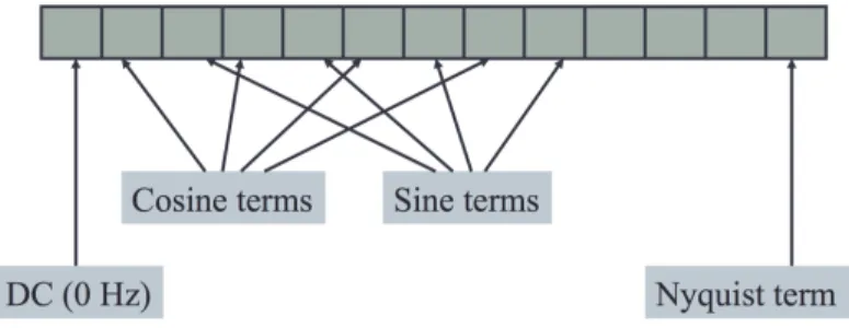
x=0 xisin(2πki/N)Recall from the discussion of the spectral centroid that when we take FFTs in Nyquist, the spectra appear as floating point arrays. As shown in Figure1, the first element of the array (index 0) is the DC (0 Hz) component1, and then we have alternating cosine and sine terms all the way up to the top element of the array, which is the cosine term of the Nyquist frequency. To visualize this in a different way, in Figure2, we represent the basis functions (cosine and sine functions that are multiplied by the signal), and the numbers here are the index in the array. The second element of the array (the blue curve labeled 1), is a single period of cosine across the duration of the analysis frame. The next element in the array is a single sine function over the length of the array. Proceedings from there, we have two cycles of cosine, two cycles of sine. Finally, the Nyquist frequency term hasn/2 cycles of a cosine, forming alternating samples of -1, +1, -1, +1, .... (The sine terms at 0 and the Nyquist frequencyN/2 are omitted because sin(2πki/N) =0 ifk=0 ork=N/2.)
Figure 1: The spectra as floating point arrays in Nyquist.
Figure 2
Following the definition of the Fourier transform, thesebasis functionsare multiplied by the input signal, the products are summed, and the sums are the output of the transform, the so-called Fouriercoefficients. Each one of the basis functions can be viewed as a frequency analyzer—it picks out a particular frequency from the input signal. The frequencies selected by the basis functions areK/duration, where indexK∈ {0,1, ...,n/2}.
Knowing the frequencies of basis functions is very important for interpreting or operating on spectra. For example, if the analysis window size is 512 samples, the sample rate is 44100 Hz, and value at index 5 of the spectrum is large, what strong frequency does that indicate? The duration is 512/44100=0.01161 s, and from
1This component comes from the particular case whereω=0, so cosωt= 1, and the integral is effectively computing the average value of
the signal. In the electrical world where we can describe electrical power as AC (alternating current, voltage oscillates up an down, e.g. at 60 Hz) or DC (direct current, voltage is constant, e.g. from a 12-volt car battery), the average value of the signal is the DC component or DC offset, and the rest is “AC.”
Figure2, we can see there are 3 periods within the analysis window, soK=3, and the frequency is 3/0.01161=
258.398 Hz. A large value at array index 5 indicates a strong component near 258.398 Hz.
Now, you may ask, what about some near-by frequency, say, 300 Hz? The next analysis frequency would be 344.531 Hz atK=4, so what happens to frequencies between 258.398 and 344.531 Hz? It turns out that each basis function is not a perfect “frequency selector” because of the finite number of samples considered. Thus, intermediate frequencies (such as 300 Hz) will have some correlation with more than one basis function, and the discrete spectrum will have more than one non-zero term. The highest magnitude coefficients will be the ones whose basis function frequencies are nearest that of the sinusoid(s) being analyzed.
1.2
Perfect Reconstruction
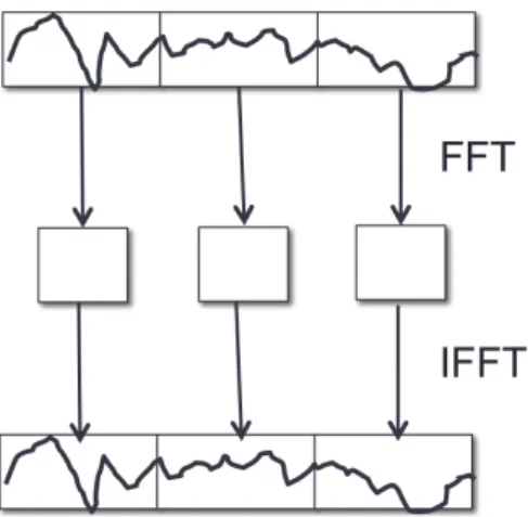
Is it possible to go from the time domain to the spectral domain and back to the time domain again without any loss or distortion? One property that works in our favor is that the FFT is information-preserving. There is a Fast Inverse Short-Time Discrete Fourier Transform, or IFFT for short, that converts Fourier coefficients back into the original signal. Thus, one way to convert to the spectral domain and back, without loss, is shown in Figure3.
Figure 3: One (flawed) approach to lossless conversion to the frequency domain and back to the time domain. This works fine unless you do any manipulation in the frequency domain, in which case discontinuities will create horrible artifacts.
The problem with Figure3is that if we change any coefficients in the spectrum, it is likely that the reconstructed signal will have discontinuities at the boundaries between one analysis frame and the next. You may recall from our early discussion on splicing that cross-fades are important to avoid clicks due to discontinuities. In fact, if there are periodic discontinuities (every analysis frame), a distinct buzz will likely be heard.
Just as we used envelopes and cross-fades to eliminate clicks in other situations, we can use envelopes to smooth each analysis frame before taking the FFT, and we can apply the smoothing envelope again after the IFFT to ensure there are no discontinuities in the signal. These analysis frames are usually calledwindowsand the envelope is called awindowing function.
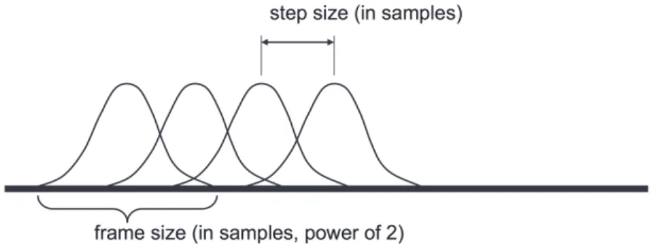
Figure4illustrates how overlapping windows are used to obtain groups of samples for analysis. From the figure, you would (correctly) expect that ideal window functions would be smooth and sum to 1. One period of the cosine function raised by 1 (so the range is from 0 to 2) is a good example of such a function. Raised cosine windows (also called Hann or Hanning windows, see Figure5) sum to one if they overlap by 50%.
But windows are applied twice: OncebeforeFFT analysis because smoothing the signal eliminates some unde-sirable artifacts from the computed spectrum, and onceafterthe IFFT to eliminate discontinuities. If we window twice, do the envelopes still sum to one? Well, no, but if we change the overlap to 75% (i.e. each window steps by 1/4 window length), then the sum of the windows is one!
With windowing, we can now alter spectra more-or-less arbitrarily, then reconstruct the time domain signal, and the result will be smooth and pretty well behaved.
Figure 4: Multiple overlapping Windows. The distance between windows is the step size.
Figure 5: The raised cosine, Hann, or Hanning window, is named after the Mathematician Von Hann. This figure, from katja (www.katjaas.nl), shows multiple Hann windows with 50% overlap, which sum to 1.
For example, a simple noise reduction technique begins by converting a signal to the frequency domain. Since noise has a broad spectrum, we expect the contribution of noise to the FFT to be a small magnitude at every frequency. Any magnitude that is below some threshold is likely to be “pure noise,” so we set it to zero. Any magnitude above threshold is likely to be, at least in part, a signal we want to keep, and we can hope the signal is strong enough to mask any noise near the same frequency. We then simply convert these altered spectra back into the time domain. Most of the noise will be removed and most of the desired signal will be retained.
2
Spectral Processing
In this section, we describe how to use Nyquist to process spectra.
2.1
From Sound to Spectra
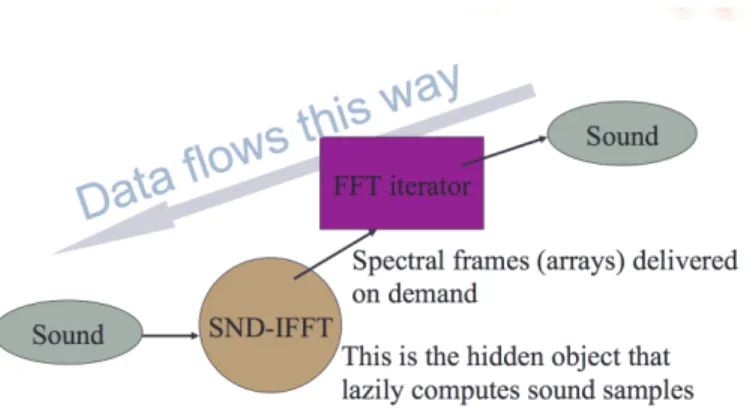
Nyquist has a built-in type for sound together with complex and rich interfaces, however, there is nothing like that in Nyquist for spectra, which are represented simply as arrays of floats representingspectral frames. Thus, we have to design an architecture for processing spectra in Nyquist (Figure6). In this figure, data flows right-to-left. We first take input sounds, extract overlapping windows, and apply the FFT to these windows to get spectral frames. We then turn those spectral frames back into time domain frames and samples, and overlap add them to produce an output sound. The data chain goes from time domain to spectral domain and back to time domain.
In terms of control flow, everything is done in a lazy or domain-driven manner, which means we start with the output on the left. When we need an output of sound, we generate a request to the object providing samples. It generates a request for a spectral frame, which it needs to do an IFFT. The request goes to the FFT interator, which pulls samples from the source sound, performs the FFT, and retuns the spectrum to SND-IFFT.
Figure 6: Spectral processing in Nyquist. Dependencies of sounds, unit generators, and objects are indicated by arrows. Computation is demand driven, and demand flows left-to-right following pointers to signal sources. Signal data flows right-to-left from signal sources to output signals after processing.
Given this simple architecture, we can insert a spectral processing object between SND-IFFT and FFT inter-ator to alter the spectra before converting them back to the time domain. We could even chain multiple spectral processors in sequence. Nyquist represents the FFT iterator in Figure6 as an object, but SAL does not support object-oriented programming, so Nyquist provides a procedural interface for SAL programmers.
The following is a simple template for spectral processing in SAL. You can find more extensive commented code in the “fftsal” extension of Nyquist (use the menu in the NyquistIDE to open the extension manager to find and install it).
To get started, we use thesa-initfunction to return an object that will generate a sequence of FFT frames by analyzing an input audio file:
set sa = sa-init(input: "./rpd-cello.wav", fft-dur: 4096 / 44100.0, skip-period: 512 / 44100.0, window: :hann)
Next, we create a spectral processing object that pulls frames as needed fromsa, applies the functionprocessing-fn
to each spectrum, and returns the resulting spectrum. The two zeros are passed toprocessing-fn, so it must take
fourparameters: the spectral analysis objectsa, the spectram (array of floats) to be modified, and two zeros.
set sp = sp-init(sa, quote(processing-fn), 0, 0)
Since SAL does not have objects, but one might want object-like behaviors, the spectral processing system is carefully implemented with “stateful” object-oriented processing in mind. The idea is that we pass state variables into the processing function and the function returns the final values of the state variables so that they can be passed back to the function on its next invocation. The definition ofprocessing-fnlooks like this:
function processing-fn(sa, frame, p1, p2) begin
... Process frame here ...
set frame[0] = 0.0 ; simple example: remove DC return list(frame, f(p1), g(p2)) ; state change end
Not thatprocessing-fnworks with state represented byp1andp2. This state is passed into the function each time it is called. The function returns alistconsisting of the altered spectral frame and the state values, which are saved and passed back on the next call.
play sp-to-sound(sp)
Thesp-to-soundfunction takes a spectral processing object created bysp-init, calls it to produce a sequence of frames, converts the frames back to the time domain, applies a windowing function, and performs an overlap add.
3
Acknowledgments
Thanks to Shuqi Dai and Sai Samarth for editing assistance.
Portions of this work are taken almost verbatim from Music and Computers, A Theoretical and Historical Approach(http://sites.music.columbia.edu/cmc/MusicAndComputers/) by Phil Burk, Larry Polansky, Douglas Repetto, Mary Robert, and Dan Rockmore. Other portions are taken almost verbatim fromIntroduction to Computer Music: Volume One(http://www.indiana.edu/~emusic/etext/toc.shtml) by Jeffrey Hass. I would like to thank these authors for generously sharing their work and knowledge.