arXiv:2004.08723v1 [eess.SP] 18 Apr 2020
PREDICTING STATION-LEVEL BIKE-SHARING DEMANDS USING GRAPH CONVOLUTIONAL NEURAL NETWORK
Lei Lin NEXTRANS Center
Purdue University E-mail: [email protected]
Weizi Li
Department of Computer Science University of North Carolina at Chapel Hill
E-mail: [email protected]
Srinivas Peeta, Corresponding Author Lyles School of Civil Engineering
Purdue University E-mail: [email protected]
Introduction
A typical motorized-passenger vehicle emits about 4.7 metric tons of carbon dioxide per year [1]. In order to decrease tailpipe emissions, reduce energy consumption, and protect the environment, as of December 2016, roughly 1000 cities around the world have started using the Bike-Sharing System (BBS) [2].
While bike sharing can enhance urban mobility as a sustainable transportation mode, it has key limitations due to the effects of fluctuating spatial and temporal demands. As pointed out by many previous studies [3, 4, 5], it is commonly seen, for BSSs with fixed stations, that some stations are empty with no bikes to check out while others are full precluding bikes from being returned at those locations. For non-dock BSSs, enhanced flexibility poses even more challenges to ensure bike availability at some places and to prevent surplus bikes from blocking sidewalks and parking areas. For both types of BSSs, accurate bike-sharing demand predictions are critical. As a result, such a topic has attracted many research efforts [3, 4, 6, 7].
In particular, graph convolutional neural networks (GCNNs) have been proposed to handle this problem with promising performance [8, 9, 10, 11]. We propose a novel GCNN model using data-driven graph filter (GCNN-DDGF). The model does not require the predefinition of an adjacency matrix, thus can be used to learn the hidden correlations among BSS stations. Two possible architectures of the GCNN-DDGF model are developed, namely GCNNreg-DDGF and GCNNrec-DDGF. The former is a regular GCNN-DDGF
model which mainly consists of two types of blocks: the convolution block and the feed-forward block. The latter captures temporal dependencies in bike-sharing demand series by introducing one more block—the recurrent block from the Long Short-term Memory (LSTM) neural network. To the best of our knowledge, this is the first study proposing a deep learning model for predicting station-level hourly demands by utilizing underlying correlations among stations.
For comparison, we use four additional GCNNs, built based on a bike-sharing graph with stations as vertices. The adjacency matrices in these GCNNs are pre-defined. To-gether, the six GCNN models as well as seven benchmark models are evaluated using the Citi BSS dataset from New York City. Our results show that the GCNNrec-DDGF
outper-forms the rest of the models, contributing to its ability to capture hidden heterogeneous correlations among BBS stations and temporal dependencies in bike-sharing demand se-ries.
GCNN with Data-Driven Graph Filter
Data-driven Graph Filter
In GCNNs, the predefinition of the adjacency matrix ˜A is not trivial. The hidden correla-tions among stacorrela-tions may be heterogeneous. Hence, it may be hard to encode them using just one kind of metric such as the Sparse Distance (SD), Demand (DE), Average Trip
Du-ration (ATD) or Demand Correlation (DC) matrix. Now, suppose the adjacency matrix ˜Ais unknown; let ˆA=D˜−12 A˜D˜
−1
2 ( ˆA∈RN×N), then we haveHl=σ(AHˆ l−1Wl)(Hl ∈RN×C),
where ˆAis called the Data-driven Graph Filter (DDGF) and is a symmetric matrix consist-ing of trainable filter parameters.
The graph filter ˆAcan be learned during the training of the deep learning model. This DDGF can learn hidden heterogeneous pairwise correlations among stations to improve prediction performance. We refer such a GCNN model as GCNN-DDGF. We can view data-driven graph filtering as filtering in the vertex domain, which avoids operations such as graph Fourier transform, filtering, and inverse graph Fourier transform.
Architecture Design
We explore two possible architectures of the GCNN-DDGF. The first, GCNNreg-DDGF, contains two types of blocks, the convolution block and the feedforward block. In the first step, through the convolution block, the signal vector at each station vertex is amplified or attenuated, and linearly combined with signals at other vertices weighted proportionally to the learned degrees of their correlations. The signal vectors become(AHˆ l−1)
i, (AHˆ l−1)j
and (AHˆ l−1)
k. In the second step, the signal vectors at the vertices of the next layer l
are calculated using the traditional feedforward block (the basic block in neural network models) to form the new signal vectors at Layer Hil, Hlj, and Hkl. The dimension of the vector at each vertex changes fromCl−1 toCl. Suppose the GCNN
reg-DDGF model has
layers from 0,1, ...tomfrom the input to the output, then, the first and second steps perform
the layer-wise calculation from layerl−1 tol,l=1, ...,m.
The second architecture, GCNNrec-DDGF imports an additional block from the Long
Short-term Memory (LSTM) neural network. The LSTM model is well-suited to capture temporal dependencies in time series data [12]. Recently, the integration of the LSTM ar-chitecture with the CNN arar-chitecture has been reported to improve large-scale taxi demand predictions by modeling both spatial and temporal relationships [13, 14]. Hence, we expect that the introduction of the recurrent block in GCNNrec-DDGF can improve
bike-sharing-demand prediction.
Model Development and Results
Citi Bike-sharing Demand Dataset
Our evaluation dataset contains over 28 million bike-sharing transactions between July 1st, 2013, and June 30th, 2016, from Citi BSS in New York City [15]. Each transaction record includes information such as trip duration, bike check out/in time, start and end station names, start and end station latitudes/longitudes, user ID, and user type (i.e., Customer or Subscriber).
Data Processing
Suppose the bike-sharing demands for all stations in houri arexi∈RN. Then, using the
demand from the previousC0−1 hours, we can construct a feature matrix Xi∈RN×C0, Xi= [Xi−C0+1, ...,Xi], and the corresponding target vectoryi+1∈R
N which represents
bike-sharing demands of all stations in the next hour. The original training dataset is transferred into paired records (X,y). The Min-Max normalization is applied to scale the data to the
range of 0 to 1. Some previous studies regarding short-term demand forecasting have shown that utilizing latest-demand information is sufficient to generate accurate predic-tions [13, 16].
We have built six GCNN models based on how the adjacency matrix of them is gener-ated. These models are referred to as GCNN-SD, GCNN-DE, GCNN-ATD, GCNN-DC, GCNNreg-DDGF, and GCNNrec-DDGF. Their performance is evaluated using the Root
Mean Square Error (RMSE) as the main criterion: RMSE =qM1∗N∑ M
i ∑Nj(yi j−Pi j)2,
whereM is the number of hours,N is the number of stations, andPi j and yi j are the
pre-dicted and recorded bike demands in hourifor station j, respectively.
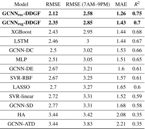
Model RMSE RMSE (7AM–9PM) MAE R2
GCNNrec-DDGF 2.12 2.58 1.26 0.75
GCNNreg-DDGF 2.35 2.85 1.43 0.7
XGBoost 2.43 2.95 1.44 0.68
LSTM 2.46 3 1.44 0.67
GCNN-DC 2.5 3.02 1.53 0.66
MLP 2.51 3.05 1.51 0.65
GCNN-DE 2.67 3.21 1.6 0.61
SVR-RBF 2.67 3.25 1.57 0.61
LASSO 2.7 3.27 1.65 0.6
SVR-linear 2.72 3.31 1.52 0.59
GCNN-SD 2.77 3.31 1.68 0.58
HA 3.44 3.42 2.08 0.35
GCNN-ATD 3.44 3.83 2.21 0.35
Table 1: Comparison in model performance using the test dataset.
We show the model performance in Table 1. In addition to RMSE, Mean Absolute Error (MAE) and R2 are used for evaluation. We calculate RMSE over the period 7AM to 9PM, since bike-sharing demands over other time periods are mostly zero or close to
zero. As a result, GCNNrec-DDGF performs the best under all measures. It has the lowest
RMSE (2.12), RMSE (7AM–9PM) (2.58), and MAE (1.26), and the highest R2 (0.75). GCNNreg-DDGF performs the second best, which indicates that the design of DDGF and
the usage of the recurrent block from LSTM are effective.
The performance of the two GCNN-DDGF models are followed by XGBoost and LSTM. While XGBoost is not designed to capture temporal dependencies in the bike-sharing demand series or the hidden correlations among stations, it supports fine-tuning and regularization for preventing overfitting [17]. LSTM performs closely to XGBoost by utilizing temporal dependencies in the bike-sharing demand series. The next best perfor-mance is from GCNN-DC, in which the pre-defined adjacency matrix with the Pearson Correlation Coefficient makes it the best among the four GCNNs with pre-defined adja-cency matrices. The GCNN-ATD model performs the worst, and has the largest RMSE (3.44), RMSE (7AM–9PM) (3.83), and MAE (2.21), and the lowest R2 (0.35). This indi-cates that ATD is not suitable for a graph adjacency matrix. It also shows that the quality of the adjacency matrix has a huge impact on the performance of the GCNN model. The remaining benchmark models perform poorly as they do not factor correlations among sta-tions or temporal dependencies in time series.
Conclusion and Future Research Directions
We have proposed a novel GCNN-DDGF model for station-level hourly demand prediction in a large-scale bike-sharing network. Different from the state-of-the-art CNN model, the GCNN model does not require data to have a regular grid structure. Consequently, it can be used to address many graph-based problems including transportation-related applications. We have implemented four GCNN models with adjacency matrices from multiple BSS data such as the SD, DE, ATD, and DC matrices. Furthermore, we have explored two architec-tures: GCNNreg-DDGF and GCNNrec-DDGF. Both models can address the limitations
of GCNN, which performance relies on a pre-defined graph structure. GCNNrec-DDGF
also implements the Long Short-term Memory (LSTM) neural network for capturing the temporal dependencies in bike-sharing demand series.
The six GCNN models and seven other benchmark models are built and evaluated using the Citi BSS dataset from New York City, which includes over 28 million transactions from 2013 to 2016. RMSE, MAE, and R2are used as measuring criteria. Our results show that GCNNrec-DDGF performs the best under all measurements, followed by GCNNrec-DDGF.
GCNN-ATD performs the worst. This observation confirms the insight from previous stud-ies, which states that the performance of GCNN depends heavily on the pre-defined struc-ture of the graph.
In future research, first, we would like to consider more factors such as weather and so-cial events (holidays and sports games). These variables can be concatenated with the input layer of the feedforward block of GCNN-DDGF. Second, the current model can be modi-fied to be an online, real-time algorithm in order to process mobile traffic data [18]. Third,
we would like to test our model on other transportation problems such as subway station de-mand prediction, and network-wide traffic state estimation and reconstruction [19, 20, 21]. Fourth, it would be useful to derive a model that can learn a sparse graph filter captur-ing directional relationships among bike-sharcaptur-ing stations. Finally, we are interested in using GCNN-DDGF to enhance the heterogeneity and accuracy of traffic simulation mod-els [22, 23] and to study the interplay between the bike-sharing system and connected and autonomous vehicles in a city [24].
References
[1] U. EPA, “Emission facts: Greenhouse gas emissions from a typical passenger vehi-cle,” 2005.
[2] J.-R. Lin, T.-H. Yang, and Y.-C. Chang, “A hub location inventory model for bicycle sharing system design: Formulation and solution,”Computers & Industrial Engineer-ing, vol. 65, no. 1, pp. 77–86, 2013.
[3] L. Chen, D. Zhang, L. Wang, D. Yang, X. Ma, S. Li, Z. Wu, G. Pan, T.-M.-T. Nguyen, and J. Jakubowicz, “Dynamic cluster-based over-demand prediction in bike sharing systems,” inProceedings of the 2016 ACM International Joint Conference on Perva-sive and Ubiquitous Computing, pp. 841–852, 2016.
[4] Y. Li, Y. Zheng, H. Zhang, and L. Chen, “Traffic prediction in a bike-sharing system,” in Proceedings of the 23rd SIGSPATIAL International Conference on Advances in Geographic Information Systems, pp. 1–10, 2015.
[5] X. Zhou, “Understanding spatiotemporal patterns of biking behavior by analyzing massive bike sharing data in chicago,”PloS one, vol. 10, no. 10, 2015.
[6] A. Rixey, “Station-level forecasting of bikesharing ridership: station network effects in three us systems,” Transportation research record, vol. 2387, no. 1, pp. 46–55, 2013.
[7] A. Faghih-Imani, N. Eluru, A. M. El-Geneidy, M. Rabbat, and U. Haq, “How land-use and urban form impact bicycle flows: evidence from the bicycle-sharing system (bixi) in montreal,”Journal of Transport Geography, vol. 41, pp. 306–314, 2014. [8] D. Shuman, S. K. Narang, P. Frossard, A. Ortega, and P. Vandergheynst, “The
emerg-ing field of signal processemerg-ing on graphs: Extendemerg-ing high-dimensional data analysis to networks and other irregular domains,”IEEE signal processing magazine, vol. 30, no. 3, pp. 83–98, 2013.
[9] J. Bruna, W. Zaremba, A. Szlam, and Y. LeCun, “Spectral networks and locally con-nected networks on graphs,”arXiv preprint arXiv:1312.6203, 2013.
[10] A. Sandryhaila and J. M. Moura, “Discrete signal processing on graphs,”IEEE trans-actions on signal processing, vol. 61, no. 7, pp. 1644–1656, 2013.
[11] T. Kipf and M. Welling, “Semi-supervised classification with graph convolutional networks,”arXiv preprint arXiv:1609.02907, 2016.
[12] S. Hochreiter and J. Schmidhuber, “Long short-term memory,”Neural computation, vol. 9, no. 8, pp. 1735–1780, 1997.
[13] J. Ke, H. Zheng, H. Yang, and X. M. Chen, “Short-term forecasting of passenger demand under on-demand ride services: A spatio-temporal deep learning approach,”
Transportation Research Part C: Emerging Technologies, vol. 85, pp. 591–608, 2017. [14] H. Yao, F. Wu, J. Ke, X. Tang, Y. Jia, S. Lu, P. Gong, J. Ye, and Z. Li, “Deep multi-view spatial-temporal network for taxi demand prediction,” in Thirty-Second AAAI Conference on Artificial Intelligence, 2018.
[15] C. B. NYC, “Citi bike system data. https://www.citibikenyc.com/,” 2017.
[16] E. Vlahogianni, M. G. Karlaftis, and J. C. Golias, “Spatio-temporal short-term urban traffic volume forecasting using genetically optimized modular networks,” Computer-Aided Civil and Infrastructure Engineering, vol. 22, no. 5, pp. 317–325, 2007. [17] L. Zhu, J. Gonder, and L. Lin, “Prediction of individual social-demographic role based
on travel behavior variability using long-term gps data,”Journal of Advanced Trans-portation, vol. 2017, 2017.
[18] L. Lin, W. Li, and S. Peeta, “Efficient data collection and accurate travel time estima-tion in a connected vehicle environment via real-time compressive sensing,”Journal of Big Data Analytics in Transportation, vol. 1, no. 2, pp. 95–107, 2019.
[19] W. Li, D. Nie, D. Wilkie, and M. C. Lin, “Citywide estimation of traffic dynamics via sparse GPS traces,”IEEE Intelligent Transportation Systems Magazine, vol. 9, no. 3, pp. 100–113, 2017.
[20] W. Li, D. Wolinski, and M. C. Lin, “City-scale traffic animation using statistical learn-ing and metamodel-based optimization,” ACM Trans. Graph., vol. 36, pp. 200:1– 200:12, Nov. 2017.
[21] W. Li, M. Jiang, Y. Chen, and M. C. Lin, “Estimating urban traffic states using iter-ative refinement and wardrop equilibria,”IET Intelligent Transport Systems, vol. 12, no. 8, pp. 875–883, 2018.
[22] D. Wilkie, J. Sewall, W. Li, and M. C. Lin, “Virtualized traffic at metropolitan scales,”
[23] Q. Chao, H. Bi, W. Li, T. Mao, Z. Wang, M. C. Lin, and Z. Deng, “A survey on vi-sual traffic simulation: Models, evaluations, and applications in autonomous driving,”
Computer Graphics Forum, vol. 39, no. 1, pp. 287–308, 2019.
[24] W. Li, D. Wolinski, and M. C. Lin, “ADAPS: Autonomous driving via principled simulations,” inIEEE International Conference on Robotics and Automation (ICRA), pp. 7625–7631, 2019.