The Applicability Analysis of the Network System Reliability and Uncertainty Calculated By Using Stochastic Simulation Algorithm

The Applicability Analysis of the Network System Reliability and Uncertainty

Calculated By Using Stochastic Simulation Algorithm

Jing Cao, Meining Zhu

School of Mathematics and Information Science & Technology Hebei Normal University of Science & Technology

Hebei, 066004, China Xuefeng Xing

Northeast Petroleum University at Qinhuangdao Hebei, 066004, China

[email protected]

ABSTRACT: There were two calculation methods of network system reliability: stochastic simulation algorithm and the analytical method. This paper performed stochastic simulation to a certain system on the uncertainty of its reliability degree applying random simulation algorithm and, meanwhile to the probability density distribution, point estimation and confidence interval of the reliability, which has proved the validity of stochastic simulation algorithm when analyzing the reliability and uncertainty of network system. What’s more, the method was verified as capable of getting more information of the system.

Keywords: Large network, Stochastic simulation algorithm, Network system reliability

Received: 14 August 2016, Revised 20 September 2016, Accepted 29 September 2016

© 2016 DLINE. All Rights Reserved

1. Introduction

and afterwards, explained the method of stochastic simulation algorithm calculating reliability of network system. At last, we proved the practicability of the stochastic simulation algorithm through experimental analysis.

2. The Concept of Stochastic Simulation Algorithm

2.1 The Application of Stochastic Simulation Algorithm

Stochastic simulation algorithm can also be known as Monte Carlo method [2-3], and has been very widely applied in engineering, mathematics calculation, physical model and many other fields.

When stochastic simulation algorithm calculates, it constantly generates different time sequence according to assumed random process, and studies the characteristics of its distribution by calculating statistics and parameter estimator, for example, if there is a large network system, and the reliable characteristic of each unit in the system is known, but its complication makes it difficult to build and calculate mathematical model[4-6], then we can calculate the predicted value of the system reliability using stochastic simulation algorithm, and when in the calculation, the accuracy of the calculation results will continuously increase with the increase of the number of stochastic simulation. As it needs to simulate and generate time series continually, so when stochastic simulation algorithm is used, it often requires high speed computer. So the stochastic simulation algorithm hasn’t been widely used until recent years.

2.2 The introduction of stochastic simulation algorithm

Assume that the reliability of each unit in network system is p_i = (i = 1, 2...n), and respectively generate a random number ri _{= (i}

= 1, 2...n) which is evenly distributed between 0 ∼ 1, when ri _{> p}i_{, the unit is considered as failed, otherwise, it is reliable, and then}

determine whether network is connectivity after eliminating failure unit. Generate a batch of random number and determine whether the network is connected during each test, when test base N is large enough, the reliability of the system can be calculated.

Rs ₌ Nc

N (1)

In the equation, N_C is the number of network connectivity being available during the experiment.

3. The Analysis of Stochastic Simulation Algorithm

3.1 The accuracy of algorithm

When stochastic simulation algorithm is computing, the arithmetic mean value is thus the approximation of E (X) can be obtained, and therefore the error of algorithm can be calculated according to central limit theorem. If limited non-zero variance of the random variables X,,,,,,,X_n is R₂ when the number of random sampling N is large enough, the equation (2) is fulfilled,

X N _{= 1}

N E N

X i

(

P | X_N - E(X)| < KAR

√

N Q0

K A_e

t2

2

dt = 1 - A

)

U

_√

_2P 2 (2)

Therefore, E = is the algorithm error threshold. Of which A is confidence, K_A can be determined by the standard normal distribution tables, R value cannot be obtained directly, but can be substituted with estimated value

K_AR

√

N

Λ

√

1 N

N

i=1

E X i2-

(

1 N E

N

X i

)

2

Thus when calculate the reliability, we can also calculate

_R

ˆ

, and conclude the error. On the other hand, we can also according to the actual demand of accuracy demand and confidence to forecast the needed algorithm simulation times N.

3.2 Efficiency of algorithm

Assume that the number of units contained in the network system is n, the worst time complexity in each sampling test is O (n), total complexity is O (N*n), when the calculation accuracy and confidence interval is determined, N is constant, so to the scale of network n in time complexity, the algorithm is a fairly efficient linear algorithm.

3.3 Algorithm analysis

Through analytic method, we conclude that unit probability importance of the network system unit i is a constant to pi :

5P_S I_prob,i , =

5P_i = $R_S

$P_i (3)

At first, we calculate reliability of network system S as Rs, then we assume reliability of unit as 1, form a new system S, and get

its reliability R . Considering the difference between system S S and S is that the reliability of the unit is different, the reliability

test of network system SS can is performed on the basis of S. From equation (3) and (1), we get:

i

S

I_prob,i = S

i

R -R_S

1-P_i = E k=1 N R S, k i N N kE=1 S, k

R N 1-P_i = 1 N N E

k=1

(

S, k

Ri - R _{S, k}

)

1-P_i

(4)

If we get the value of in the kth _{reliability test, we get the value |} prob,i_{. Considering in the k}th _{random simulation, unit} i of network system S_i won’t be invalid; network system S and S_i are the same except for i. Set system S, S_i after eliminating the failure unit network as Sc_{, S}ci_{, then}

R i S, k_{- R}S,k

R_Sc,_k- R_S,k =

{

1 unit i is invalid and S_C is not connect, S_a

0

(5)

Substitute equation (5) into equation (4), we can get:

I_prob,i =

1 N

N

E

k=1

(

R i

S, k - R S, k

)

1-P_i =

N_i

N(1 - P_i) (6)

In the equation, Ni is the number of reliability stochastic simulation experiment, S Ci is the number of times when unit i fails and

network Sc can not connect and the number of connected network S.

4. The Uncertainty Analysis of Stochastic Simulation

4.1 The uncertainty of propagation law synthetic method evaluation

A certain physical quantity Y which represents the system (according to the calculation or measurement) is usually determined by the other N components of the system or N inputs X₁, X₂,...X_N thus we get Y = f (X, X₂,... X_N). If the inputs X₁, X₂,...X_N are noninterference, then expand function f, according to the standard uncertainty u (X_i) of X_i, we can get system synthesis standard uncertainty uc (Y), we get:

N

u2

c(Y) =

Σ

i=1

(∂ f

∂X_i ) 2 _u2₍

X_i) (7)

For Y = f (X₁, X₂, ....X_N), , we lead in vector X = (X₁, X₂,...,X_N), then Y can be expressed as Y = f (x). If the distribution of weight Xi _{and function relation f are given, we can use the distribution of each component to simulate the distribution of computing}

systems. The method is as follows: from stochastic simulation sampling X, we get M group xk_{, and then the corresponding value}

of Y. By sampling, we get from sampling:

x_k = (x_1k, x_2k,....x_Nk)

y_k = (X_1k, X_2k,....X_Nk)

In the equation, K = 1, 2,..., M. Form the distribution of Y through yk_{, and through the distribution of Y we get the best value of}

y and standard uncertainty u (Y) of Y.

(8)

(9)

y = 1

M

Σ

M

k=1

y_{K (10)}

u(Y) =

√

1

M - 1

Σ

M

k=1

(y_k - y)2 (11)

From the above processes, we know that if the Monte Carlo method is used to simulate system uncertainty, it must fulfill two conditions: one is to analyze the parameters of characterization system and get mathematical model for describing the system ultimate parameter; the other one is to understand the distribution which input parameters obey in the mathematical model.

4.3 The calculation of system reliability empirical distribution function and the confidence interval

According to the definition of empirical distribution function, set ξ means a random variable, and the distribution function is F(x). Then, to perform n times repeated independent trials to ξ, v_n (x) means the occurrences number of random events {ξ <x } in n times of repeated and independent observations, namely the number of times when the value among n times observations x₁,

x₂,..., x_n is less than x. The empirical distribution function of general ξ is:

(12)

Differential of empirical distribution function is empirical distribution density function, the specific algorithm is as follows: We searched for the maximum ymax _{and minimum y}min _{of samples, among M samples we get from M times of simulations, and}

divide [ymin_{, y}max _{] into m}

0 intervals, interval of each interval is

Δm_r=

Σ

N

φ _j(y_j) ₍₁₃₎

(14)

Then the distribution density function of system stochastic variable is:

j=1

fΛ(y_r) =_ΔΔmr

Assume that samples yk _{represents a series of reliability value obtained from simulative calculation, and arrange y}k _{from small to}

large, we get:

y_S(1) ≤ _y S

(2) ≤ _{.... y} S

(k) ≤ ....≤ _y S

(N)

As P(y > y_S(k) ≈ 1 − , we can approximate think the confidence lower limit of y in the confidence level (1-k/N) is y_S(k)_{. Set fixed}

confidence level as p, such as p = 0.95, through the (1- p) / 2 quantile of yk_{,we can get the lower end y}

low of the inclusion interval;

through the (1 + p) / 2 point of yk_{, we can get the up end y}high _{of the inclusion interval. Take the confidence level as p (p = 0.95),}

the inclusion interval CI of Y is [y_low ,yhigh_].

5.Simulation Test

5.1 An example of large-scale complex networks

(16) k

N

Figure 1. The urban road grid system diagram

Figure 1 is the road network system of a city, and the network system is a large complex network system which is composed by 1293nodes and 760 edges. Set the reliability of cross unit as 0.9, the reliability of each section unit as 0.70. Through 10 million times simulation, and the connected reliability is 0.78975 obtained by this algorithm, importance value of unit probability is represented with the width of the different road unit in the figure, the wider the width is, the more important the unit is. From figure 1, we see that because the city road network is divided into two parts, which makes the probability importance degree of the few roads and cross which connects the two parts few higher than the other roads and cross within that section. The calculation results are consistent with the actual situation, which fully shows the effectiveness of random simulation method in the large-scale network.

5.2 The comparison between stochastic simulation algorithm and ORDED algorithm in network reliability calculation

Figure 2 is a simple network which includes 5 nodes, and 8 connections. Numbers on each line segment shows the probability of the connection being under failure mode, and is marked as Li_{(l = 1,2... 8). If L}i _{is very small, the network has high reliable}

components. Both methods can be applied to the network to calculate connectivity reliability of nodes 1 and 5 in Figure 2. The application of stochastic simulation algorithm is as follows:

(1) Xi _{(l = 1, 2... 8) is randomly given. Each connection in the network with X}i _{< L}i _{is deleted, otherwise preserved.}

Figure 2. Simple network

(3) Repeat step 1 and step 2 for each simulation, if there are m simulations, then the final connectivity reliability is: .

Σ

Ci

m

The application of ORDER algorithm is as follows:

(1) given A = {S1_{, S}2_{,..., S}m_{} : A includes m possible states, and arranges in descending sequence as P (S}1₎ ≥ _{P (S}2₎ ≥ _..≥ _P(Sm_).

(2) Check the reliability Ci _{of each state, if it is still connected, C}i _{= 1, otherwise C}i _{= 0.}

(3) The final connectivity reliability is: [C_i × P (S_i)].

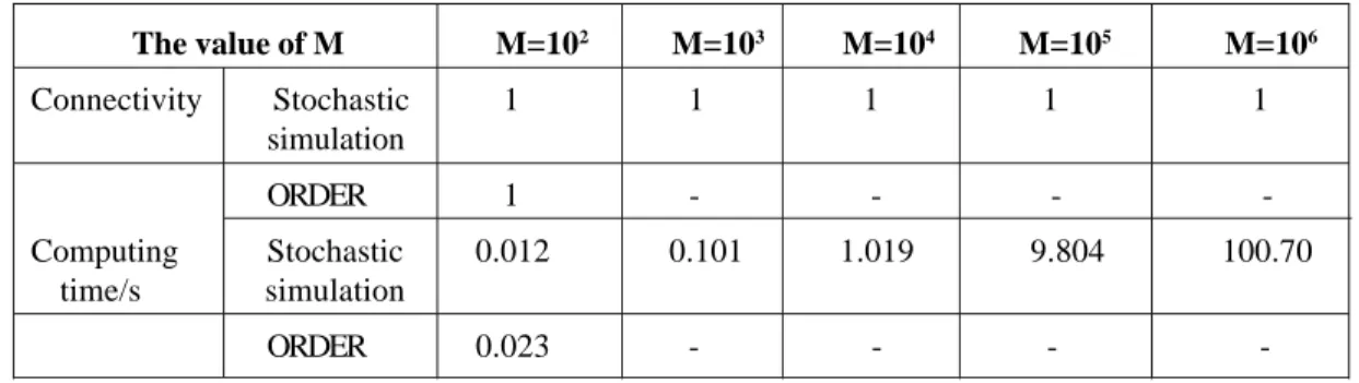
The results are shown in table 1. The calculation was finished by a computer allocated with CPU of 3100 MHZ. Although there are only eight connections in the network, the total number of state has reached 28 = 256, so only the former 100 state of ORDER algorithm was considered. The results shows that the connectivity reliability between nodes 1 and 2 is 1, therefore, we believed that the two nodes were always connected. Because the network is small, it is difficult to see the difference between the two methods; so the next step is to apply them to a larger network.

The value of M M=102 _M=103 _M=104 _M=105 _M=106

Connectivity Stochastic 1 1 1 1 1 simulation

ORDER 1 - - - -Computing Stochastic 0.012 0.101 1.019 9.804 100.70 time/s simulation

ORDER 0.023

Σ

Table 1. The connectivity reliability of node 1 and node 5 in figure 2

For a medium-sized network, there are a total of 558 nodes and 740 links, thus the network has 2740 _{states. This is a large number,}

and it’s impossible to enumerate all the network states. We can only enumerate m major states, the approximate total connectivity of the network is:

C ≈

Σ

i=1 m

C _i • P_i (17)

Here, Pi _{is the possibility of the i}th _{network state; C}i _{is the connectivity of the i}th _{network state.} C_2n≤ C_i ≤ C₁ ; i = 1,2,...2n

Here, Ci _{is the connectivity of all the connections in a controllable state; C}2n _{is the connectivity of all the connections in failure}

conditions. Therefore, Ci _{= 1, C}2n_{= 0.}

If take m main possible states into consideration, then:

Σ

C =

m

C_i • P_i+

Σ

i=1

2n i=m+1

C_i • P_{i (19)}

We get that from equation (18):

Σ

i=m+1

2n

C ₂n•

P_i≤

Σ

2

n

i=m+1Ci • Pi≤

Σ

2n

C₁ • P₁ (20)

As Ci _{= 1, and C}2n _{= 0 the equation (20) can be changed to:} i=m+1

Σ

Σ

2n

C_i • P_{i ≤}

Σ

2n

P_i= 1 -

Σ

i=1

m

p_{i (21)}

Substitute equation (21) into equation (19), and we get: 0 ≤

i=m+1 i=m+1

Σ

Σ

m

i=0

C_i • P_i ≤ C≤

i=0

m

C_i • P_i + 1

-i=1

m

p_{i (22)}

A and B are the two distant places of the medium-sized network, which are located on the road of the south and the north, and both network connectivity degrees are shown in table 2. When consider the 102 _{major state, the range is changed into [0.785 2,}

0.860 7]. With the increase of m, the upper and lower boundary of range C converges quickly. When m is 106_{, the range is [0.860}

1, 0.860 6], so it can be said that the connectivity between A and B is 0.86.

The value of M M=102 _M=103 _M=104 _M=105 _M=106

_{Connectivity Stochastic 1 1 0.999 0.999 0.999} simulation

ORDER [0.785, 0.860] [0.85, 0.86] [0.85,0.86] [0.85, 0.86] [0.86, 0.86]

Computing Stochastic 3.609 9.038 71.41 636.5 6259 time/s simulation

ORDER 3.116 9.859 83.86 1229 89029

Table 2. Connectivity reliability of a and b in a medium-sized network

On the other hand, when use the Monte Carlo method, the results will be converged very slow. When m = 106_{, the connectivity}

is 0.9999 which is much bigger than the real value 0.86. As for the computing time, Monte Carlo method is much faster than ORDER algorithm. When m = 106_{, computation time the former algorithm is 6, 259 s, the latter is 89 029 s.}

6. Conclusion

compared with the algorithm according to propagation law, can get more information of the system uncertainty and when the system composition is complicated, Monte Carlo method is simple and practicable both from the view of principle and practical operation. However, if only the uncertainty of sub-system(or component) is available while the distribution situation of the uncertainty of each component is unknown, Monte Carlo method is not applicable.

In short, the stochastic simulation algorithm of network reliability has many advantages. With further development of computer technology, stochastic simulation algorithm will play an important role in reliability computing of network system [7-10].

References

[1] Rosenthal, A. (1977). Computing the reliability of complex network, SIAM J Appl Math, 32 (2) 410-421.

[2] Fishman, G.S. (1989). Estimation the s-t reliability function using importance and stratified sampling, Operations Research, 37 (4) 462-473.

[3] Fishman, G.S. (1995). Monte Carlo: Concepts, Algorithms, and Applications, New York: Springer Verlag.

[4] Satyanarayana, A., Wood, R.K. (1985). A linear-time algorithm for computing K-terminal reliability in series-parallel networks,

Siam. J. Comput, 14 (4) 818- 832.

[5] Schanzer, R. (1995). Comment on: Reliablity modeling and performance of variable link-capacity network, IEEE Tansacitions on Reliability, 44 (4) 620-621.

[6] Spragins, J.D., Sinclair, J.C., Kang, Y.J., Jafari, H. (1986). Current telecommunication network reliability models: A critcal assessment, IEEE Journal on Selected Areas in Communications, 4 (7) 1168-1173.

[7] Strayer, H.J., Colbourn, C.J. (1997). Bounding flow-performance in probabilistic weighted networds, IEEE Transacitins on Reliability, 46 (1) 3-9.

[8] Liu, S.B., Cheng, K.H., Liu. X.P. (2000). Network reliability with node failures, Networks, 35 (2) 109-117.

[9] Malinowski, J., Preuss.W. (1997). A parallel algorithm evaluating the reliability of a system with known minimal cuts (paths),

Microelectronics Reliability, 37 (2) 255-265.