Consensus queries in ligand-based virtual screening experiments

(1)

RESEARCH ARTICLE

Consensus queries in ligand-based

virtual screening experiments

Francois Berenger

1,2*

_{, Oanh Vu}

1

_{and Jens Meiler}

1

Abstract

Background: In ligand-based virtual screening experiments, a known active ligand is used in similarity searches to find putative active compounds for the same protein target. When there are several known active molecules, screen-ing usscreen-ing all of them is more powerful than screenscreen-ing usscreen-ing a sscreen-ingle ligand. A consensus query can be created by either screening serially with different ligands before merging the obtained similarity scores, or by combining the molecular descriptors (i.e. chemical fingerprints) of those ligands.

Results: We report on the discriminative power and speed of several consensus methods, on two datasets only made of experimentally verified molecules. The two datasets contain a total of 19 protein targets, 3776 known active and ~ 2 × 106_{inactive molecules. Three chemical fingerprints are investigated: MACCS 166 bits, ECFP4 2048 bits and} an unfolded version of MOLPRINT2D. Four different consensus policies and five consensus sizes were benchmarked.

Conclusions: The best consensus method is to rank candidate molecules using the maximum score obtained by each candidate molecule versus all known actives. When the number of actives used is small, the same screening per-formance can be approached by a consensus fingerprint. However, if the computational exploration of the chemical space is limited by speed (i.e. throughput), a consensus fingerprint allows to outperform this consensus of scores.

Keywords: Similarity search, Several bioactives, Consensus query, Ligand-based virtual screening (LBVS), Chemical fingerprint, Potency scaling, MACCS, ECFP4, MOLPRINT2D, Tanimoto score

© The Author(s) 2017. This article is distributed under the terms of the Creative Commons Attribution 4.0 International License (http://creativecommons.org/licenses/by/4.0/), which permits unrestricted use, distribution, and reproduction in any medium, provided you give appropriate credit to the original author(s) and the source, provide a link to the Creative Commons license, and indicate if changes were made. The Creative Commons Public Domain Dedication waiver (http://creativecommons.org/ publicdomain/zero/1.0/) applies to the data made available in this article, unless otherwise stated.

Background

Similarity searches help expand the collection of known actives in the early stages of a drug discovery project. Interestingly, similarity searches do not require a diverse collection of active and inactive molecules prior to be used. Sometimes, in a ligand-based virtual screening (LBVS) campaign, only a limited number of active com-pounds is known. Such comcom-pounds could be found from the scientific literature, patent searches or a moderately successful structure-based virtual screen followed by wet-lab testing. This data scarcity might render standard machine learning algorithms inapplicable. Indeed, most Quantitative Structure Activity Relationship (QSAR) methods are data hungry. While expert machine learning users may benefit from recent developments [1, 2], most

users will be left in front of several questions: (a) how many actives are needed to create a powerful classifier, (b) which chemical fingerprint should be used to encode those actives, and (c) what is the best way to combine those fingerprints.

Similarity searches that exploit the chemical simi-larity principle [3] are some of the earliest techniques developed in chemoinformatics [4, 5]. When several ligands are known for a given protein target, they can be used simultaneously to better find novel, putative active molecules.

This study measures the performance and speed of several ways to combine the knowledge about known actives. We investigate the effect of the fingerprint choice, the number of actives and the method used to combine fingerprints. Compared to most previous stud-ies, our datasets are only made of experimentally verified molecules. We also evaluate the effect of scoring speed in CPU-bounded experiments, to show a potential use

Open Access

*Correspondence: [email protected]

2_{Division of System Cohort, Medical Institute of Bioregulation, Kyushu} University, Fukuoka, Japan

(2)

when screening immense virtual chemical libraries. We finally discuss which combination of fingerprint, con-sensus size and concon-sensus method gives the best perfor-mance or should be avoided.

Using multiple bioactive reference structures has been studied by several authors [6–14]. Shemetulskis et al. [6] have created modal fingerprints, where a bit is set in the consensus query if it is set in a given percentage (the mode) of known active molecules. Xue et al. [8] have used all bits consistently set in compounds of a same activity class (called consensus bit patterns) and scale factors for those bits to modify the Tanimoto score. This approach is called fingerprint scaling. It increases the probability of finding active molecules by virtual screen-ing. Wang and Bajorath [13] have used bit silencing in MACCS fingerprints to create a bit-position-dependent weight vector. This weight vector modifies the Tanimoto coefficient in order to derive compound-class-directed similarity metrics that improve virtual screening perfor-mance compared to conventional Tanimoto searches. Hert et al. [9] have compared merging several finger-prints into a single combined fingerprint, applying data fusion (merging of scores) to the similarity rankings of single queries and approximated substructure searches. Hert et al. found that merging similarity scores and using binary kernel discrimination are the most power-ful techniques. Later, Whittle [11] confirmed that fus-ing similarity scores usfus-ing the maximum score rule (or the minimum rank if scores are not available) is one of the most powerful strategies. For a recent study of data fusion methods with fragment-like molecules, see Schul-tes 2015 [14].

Ligand-based virtual screening methods have also been extended to take into account the different potency levels of known actives [10, 12]. This potency scaling technique allows to bias the search space towards the detection of increasingly potent hits [10]. To bias the search, a loga-rithmic weighting scheme based on IC50 1_{values was} introduced. Let qi be a known active molecule. qi is

assigned a weight wi given it’s IC50 value (IC50_qi) and the

IC50 value of the least active molecule (IC50min):

This logarithmic weighting scheme ensures linear scaling over the entire potency range and attributes a weight of one to the least active molecule [10]. In Vogt and Bajo-rath [12], the same weighting scheme is used to bias two distinct virtual screening algorithms and applied to a high-throughput screening (HTS) data set of cathepsin B

1 _{IC50: 50% Inhibitory Concentration. An IC50 value represents the} con-centration of a drug that is required to inhibit a given biological process by 50% invitro.

(1)

wi =log(IC50min)−log(IC50qi)+1.0

inhibitors. The authors observed that using multiple ref-erence compounds and potency scaling allows to direct the search towards detection of more potent database hits.

The pharmacologically relevant chemical space is immense. A study [15] estimates its size in the order of 1033 molecules, with up to 36 heavy atoms each. While the database of commercially-available compounds ZINC15 [16] totals 335×106 compounds as of May

2017, there are virtual chemical libraries with more than

166×109 molecules [17, 18]. Hence, one can

imag-ine scenarios where the speed of a virtual screen has its importance.

Methods

In this study, only fully automatic methods are investi-gated on 2D fingerprints. None of these methods requires fitting to a training set. The investigated methods are all parameter-free. Implicit parameters, if any, are detailed.

Datasets

Several protein targets coming from two distinct datasets were used. None of those datasets contain any decoy (i.e. molecules that have not been experimentally verified as either active or inactive). A decoy is a supposedly inac-tive, computationally engineered [19] or randomly cho-sen [8] molecule. Hence, in this study there is no risk that a decoy creation protocol can be reverse engineered by any of the evaluated methods. Also, some of the datasets used are real world examples since they come from HTS campaigns.

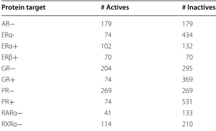
Our first dataset is the manually curated nuclear recep-tors ligands and structures benchmarking database [20] (NRLiSt BDB2_{). The NRLiSt is an exhaustive,} NR-focused, benchmarking database. The original NRLiSt contains 9905 ligands and 339 protein targets. However, for the specific needs of this study, the NRLiSt was fur-ther filtered in order to contain only protein targets for which there are at least 40 known actives and at least the same amount (or more) of tested inactives. Furthermore, only active molecules with an IC50 value are accounted for. A summary of this dataset is given in Table 1.

The second dataset, MLQSAR,3_{is a compilation of} vali-dated PubChem High Throughput Screens [21]. PubChem provides libraries of small molecules that have been tested in HTS experiments. This dataset focuses on experiments with a single well-defined and pharmaceuti-cally relevant protein target. A target is only retained if it has at least 150 confirmed active compounds. A sum-mary of MLQSAR is given in Table 2. For several targets,

2 _{http://nrlist.drugdesign.fr.}

(3)

active molecules just have a flag and no IC50 data. There are only two targets (PubChem SAID 485290 and 435,008) for which activity values span several orders of magnitude, while this is the case for all NRLIST targets.

Fingerprints

In this study, three different fingerprints were used. The MACCS 166 bits fingerprint as provided by Open Babel [22]. The ECFP4 2048 bits fingerprint as provided by Rdkit [23, 24] and an unfolded MOLPRINT2D [25, 26] implementation, referred to as UMOP2D in the text. MOLPRINT2D descriptors encode atom environment based on SYBYL atom types (i.e. atom type and hybridi-zation state) derived from the molecular graph. Only heavy atoms and their connected neighbors up to a dis-tance of two bonds are considered by this fingerprint. MOLPRINT2D will be available in the upcoming version of the Bio Chemical Library [27]. The goal of this study is not to compare the power of individual fingerprints; see Sastry [28] for an extensive comparison.

Chemical similarity

To fairly compare methods during experiments, the Tani-moto score is used consistently. Given two binary finger-prints A and B of equal length:

Given two fingerprints X and Y encoded as vectors of floats of length N:

Performance metrics and curves

To assess overall classifier performance, the Area Under the receiver operating characteristic Curve (AUC) is used. To measure early retrieval performance, the Power Metric at 10% (PM10%) is used [29]. The power metric is a function of the True Positive Rate (TPR) and False Posi-tive Rate (FPR) at a given threshold. The power metric is statistically robust to variations in the threshold and ratio of active compounds over total number of compounds in a dataset. At the same time, the power metric is also sen-sitive to variations in model quality.

In some experiments, the accumulated number of actives is drawn. This curve is obtained by walking down a rank-ordered list of compounds (the X axis lists ranks of data-base molecules) and plotting on the Y axis the number of active molecules encountered so far.

Consensus policies

In all methods described hereafter, there is no parame-ter fitting to any of the datasets. Also, no training using known actives and inactives is required prior to applying any of the methods.

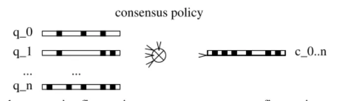
A consensus query is formed by the combination of a set of query molecules (also called known actives) while following a consensus policy. The policy specifies how fingerprints are combined (Fig. 1).

Let P be the set of all protein targets. Let p be a given protein target (p∈P).

Let M be the set of all tested molecules for p. Let fp(m) be the fingerprint of molecule m∈M. Let A be the set of active molecules on p (A⊂M). Let I be the set of inactive molecules on p (I=M\A). Let Q be a randomly selected set of actives that will be used to build a consensus query of size N (Q⊂A∧ |Q| =N). In this study, only two to 20 actives

are used to create a consensus query (2≤N ≤20).

(2)

Tani(A,B)= |A∩B| |A∪B|

(3)

Tani(X,Y)=

N i=1xiyi N

i=1x 2

i +y

2

i −xiyi

(4)

PMx%=

TPRx% TPRx%+FPRx%

Table 1 The NRLiSt subset with IC50 data for all actives

‘+’ after a target name means actives (resp. inactives) have an agonist (resp. antagonist) effect. ‘−’ after a target name means the opposite

Protein target # Actives # Inactives

AR− 179 179

ERα- 74 434

ERα+ 102 132

ERβ+ 70 70

GR− 204 295

GR+ 74 369

PR− 269 269

PR+ 74 531

RARα− 41 133

RXRα− 114 210

Table 2 The nine HTS datasets with their PubChem Sum-mary Assay ID (SAID)

Protein target class SAID # Actives # Inactives

GPCR 435008 233 217,925

1798 187 61,646

435034 362 61,394

Ion channel 1843 172 301,321

2258 213 302,192

463087 703 100,172

Transporter 488997 252 302,054

Kinase inhibitor 2689 172 319,620

(4)

Let C=M\Q be the set of candidate molecules for p;

sometimes referred to as the “database” of molecules to screen.

During a retrospective ligand-based virtual screening experiment, the active or inactive status of a molecule

ci∈C is ignored, until the final computation of a

perfor-mance metric or curve is triggered.

We call query qi a molecule randomly drawn from Q.

Let score(qi,cj)|qi ∈Q∧cj ∈C be the Tanimoto score

of the fingerprint of the query molecule at index i with the fingerprint of the candidate molecule at index j. If x is a consensus query of fingerprint type, writing score(x,cj)

is also valid.

The list of policies described hereafter are: single, pes-simist, optimist, realist and knowledgeable. Policies are sometimes abbreviated using their first four letter.

Let O be the set of all consensus policies: O= {Sing,Oppo,Pess,Opti,Real,Know}.

Let cscore(o,Q,ci) be the consensus query score using

policy o∈O and set of known actives Q with candidate molecule ci.

Single query In the single policy, each active is used in turn as the query molecule. This policy reproduces the average performance of using a single bioactive molecule as query instead of several.

Opportunist consensus of scores The score assigned to a candidate molecule is the maximum score it gets over all query molecules. This consensus query is a set of finger-prints. In the literature [9, 11], this method is classified as a data fusion method and called max of scores or mini-mum of ranks.

(5)

cscore(Sing,qi,ci)=score(fp(qi),fp(ci))

(6)

cons(Oppo,Q)=Q cscore(Oppo,Q,ci)=

max{score(fp(qi),fp(ci))∀qi ∈Q}

Pessimist The consensus query is the fingerprint result-ing from doresult-ing a bitwise AND of all query fresult-ingerprints. This consensus is a single fingerprint. This is the “consen-sus bit pattern” from Xue et al. [8].

Optimist consensus of fingerprints he consensus query is the fingerprint resulting from doing a bit-wise OR of all query fingerprints. This consensus is a single fingerprint.

Realist The consensus query is the float vector where each index i of the vector contains the probability for bit i of being set over all queries. This consensus is a single fingerprint.

Knowledgeable This consensus is almost like the real-ist consensus, except that query molecule fingerprints are potency-scaled (cf. formula 1) prior to being taken into account. This consensus is a single fingerprint.

Software

Our software, called Consent, is written in OCaml. OCaml is a statically-typed functional programming language allowing fast prototyping of scientific software [30].

We release all our software, scripts and datasets as open source. MACCS 166 bits (resp. ECFP4 2048 bits) fingerprints were computed using a small C++ program linked to Open Babel v2.4.1 (resp. RDkit v2015.03.1). MOLPRINT2D unfolded fingerprints are computed by Consent.

Consent can exploit multicore computers thanks to the Parmap [31] library. Some of the dataset preparation, running of experiments and post processing of results were accelerated by PAR [32].

(7)

x=cons(Pess,Q)= ∩{fp(qi)∀qi ∈Q}

cscore(Pess,Q,ci)=score(x,fp(ci))

(8)

x=cons(Opti,Q)= ∪{fp(qi)∀qi∈Q} cscore(Opti,Q,ci)=score(x,fp(ci))

(9) x=cons(Real,Q)=

[p(bitj=1)∀j∈bits(fp(qi))∀qi∈Q]

cscore(Real,Q,ci)=score(x,ci)

(10)

Qw=potency_scale(Q) x=cons(Know,Qw)=

[p(bitj=1)∀j∈bits(fp(qi))∀qi∈Q_w]

cscore(Know,Q_w,ci)=score(x,ci)

q_0 q_1

q_n... ...

consensus policy

known active fingerprints consensus fingerprint c_0..n

(5)

Experiments

Consensus query experiments

The size of the consensus is varied from 2 to 20 actives. Experiments don’t go over 20 actives, because it is imagi-nable that if more than twenty actives are known for a given target, one might also have many known inactives and could be training a QSAR model. Also, some protein tar-gets of our datasets only have 40 actives, so it is not allowed to use more than half of them to build a consensus query. Active molecules used to build a consensus query are ran-domly drawn from the actives of the given protein target. Actives used to build a consensus query are also removed from the database to screen. Hence, benchmarks don’t become artificially easier as the consensus size is grown.

On the NRLIST dataset, experiments are repeated at least a hundred times since this dataset is small. On the MLQSAR dataset, experiments are repeated up to 20 times. MLQSAR is quite large and calculating statistics on it is costly. When a performance curve is reported, this curve is the median curve obtained during experi-ments using the same (protein target, consensus size, consensus policy) experiment configuration triplet. Cal-culating this median curve is memory intensive, espe-cially for MLQSAR.

Speed experiments

Speed experiments were performed on PubChem SAID 485290, which contains 341,365 active and inactive mol-ecules (largest dataset). The virtual screen was run once, then the median throughput (in molecule/s) of the five subsequent runs was computed.

Experiments were performed using a single core of an Intel Xeon CPU at 3.50 GHz on a Linux CentOS v6.8 workstation equipped with 64 GB or RAM.

Potency‑scaling experiments

In potency scaling experiments, two consensus policies are compared. The database of compounds for a given target is rank ordered several times and the median rank for each active molecule with each consensus policy is recorded.

To compare two consensus policies, active molecules are first ordered by decreasing IC50, then the differ-ence of ranks between the two policies is measured. This allows to compute a delta rank plot. A negative delta rank is a positive outcome: the given active molecule went higher in the rank-ordered list of compounds (i.e. it is found earlier by the virtual screen). A positive delta rank is the opposite negative outcome.

CPU‑bounded experiments

In CPU-bounded experiments, two consensus policies are compared and the faster policy is allowed to score

more molecules. For example, if policy p1 is two times faster than policy p2. Then, p2 will only screen a random

half partition of the database while p1 will screen the whole database.

This experiment simulates an in silico combinatorial chemistry library enumeration [18, 33–36], where mol-ecules are generated, fingerprinted and scored on the fly. The virtual screen is stopped after some amount of time, not because the immense library enumeration has finished.

Results

Effect of the consensus size

Discriminative power

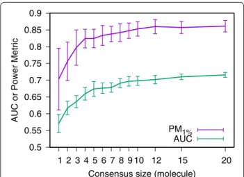
As the consensus size is growing, the power to discrimi-nate between active and inactive molecules increases.

When looking at the global performance of the classi-fier (monitored by its AUC) as well as its early recovery capability (monitored by its PM1% [29]), there is a clear improvement correlated with the growth in consensus size (Fig. 2). On this target, there is no more improve-ment in early recovery capability once a consensus of size twelve is reached. A bigger consensus only improves the AUC.

Speed

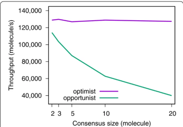
While a consensus fingerprint query screens at a con-stant speed of ~ 130,000 molecule/s (Fig. 3), this is not the case for a consensus based on scores.

Figure 3 shows a comparison of speed between the optimist and the opportunist consensus. As the number

0.5 0.55 0.6 0.65 0.7 0.75 0.8 0.85 0.9

1 2 3 4 5 6 7 8 9 10 12 15 20

AUC or Power Metri

c

Consensus size (molecule)

PM_1%

AUC

Fig. 2 Effect of the consensus size on the consensus query global classification performance (AUC) and early recovery capability (PM1%

(6)

of known actives used to build the consensus is growing, the opportunist consensus becomes slower.

Effect of the consensus policy and fingerprint type

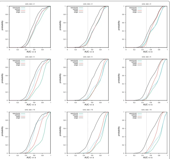
NRLIST dataset

On this dataset, results across consensus policies and fin-gerprints can be seen in Fig. 4.

For MACCS fingerprints, the most efficient policy is the opportunist, followed by the realist consensus. The optimist consensus performs less well than a single query when the AUC reached is greater than 0.85.

For ECFP4 fingerprints, the most efficient policy is also the opportunist one. Then, the realist consensus or the optimist consensus (for AUC ≥ 0.75) are the most pow-erful. With this fingerprint, all consensus policies have a better performance than a single query, as can be seen in the gap between the black curve and all other curves.

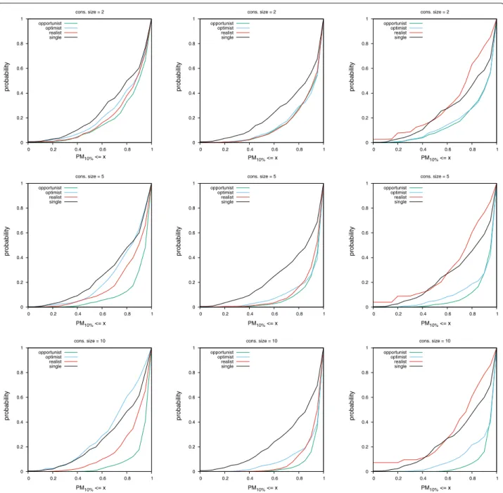
For the UMOP2D fingerprint, the trend is similar than ECFP4. However, the optimist consensus is always better than the realist one and can even outperform the oppor-tunist consensus for PM values ≥ 0.8 (Fig. 5).

The realist consensus is not shown on these AUC plots. Its performance is very similar to the realist consensus but its effect is different and shown later in “Effect of

potency-scaling” section.

Across fingerprints, the least random and best per-forming method is always the opportunist consensus. However, as the consensus size gets smaller, the spread between curves (and hence the performance difference between methods) becomes smaller.

It is interesting to observe that the trend is different for each fingerprint. If something is observed for one finger-print, it might not hold for other fingerprints.

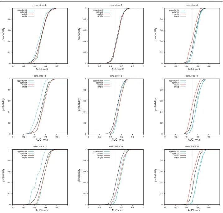
MLQSAR dataset

Results on this dataset differ from results on the NRLIST. As a general trend, the spread between curves for differ-ent consensus policies is smaller. The biggest difference is that even by looking only at AUC values, the optimist consensus on MACCS fingerprints and the realist con-sensus on UMOP2D fingerprints are clearly disqualified. They perform worse than a single query. While on the NRLIST, this observation can only be made by looking at CDF curves of PM values.

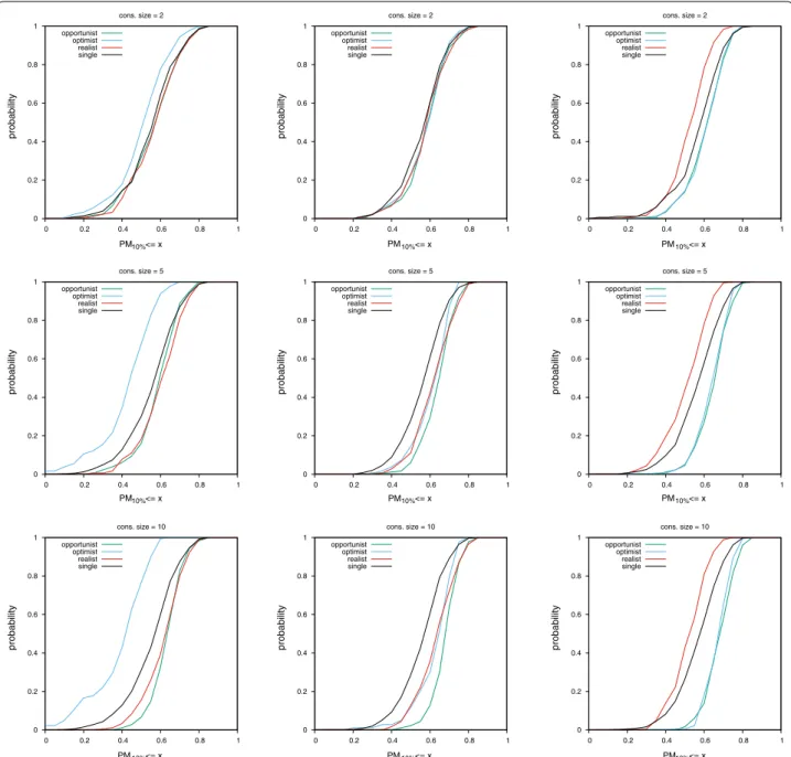
Experiments on this dataset show that combining the realist policy with the MACCS or ECFP4 fingerprints can outperform the performance of the opportunist con-sensus (left and middle columns of Figs. 6 and 7, yellow curve under all other curves).

Table 3 provides a bird’s-eye view of results shown in Figs. 4, 5, 6 and 7 (same protocol but different experiment).

Effect of potency‑scaling

The effect of potency scaling is that it brings highly active molecules closer to the query but pushes further away less potent molecules (Fig. 8).

In our experiments (Table 4) and in terms of bringing the most active molecules closer to the query, there is a clear advantage of the knowledgeable policy (which is potency scaled) versus the realist one. On the NRLIST, the knowledgeable policy is also better than the oppor-tunist one. However, on the two MLQSAR targets with a wide distribution of potency values, this behavior is observed only once.

CPU‑bounded experiments

Consensus queries using a single fingerprint can be several times faster than a consensus based on scores (Table 5). For example, a consensus query using only five actives is 1.46 times faster than a consensus of five scores. With 20 actives, it becomes 3.19 times faster.

In theory, a consensus made of N scores could be up to N times slower than a fingerprint consensus. However, our software being optimized, the slowdown is not so high.

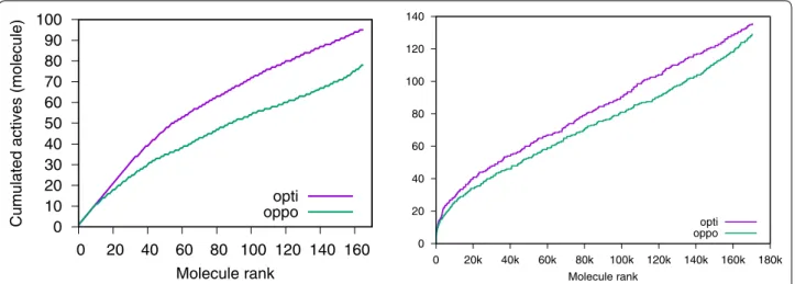
In the case where the computational exploration of the chemical space is limited by the speed at which molecules can be scored, there is an advantage at using a consensus query which is faster than a consensus of scores (Fig. 9

and Table 5). In at least six out of nine targets from the MLQSAR dataset, the optimist consensus outperforms the opportunist one in CPU-bounded experiments. On the NRLIST dataset, the same trend is observed in at least eight out of ten targets.

40,000 60,000 80,000 100,000 120,000 140,000

2 3 5 10 20

Throughput (molecule/s)

Consensus size (molecule) optimist

opportunist

(7)

Discussion

We say a consensus fingerprint degenerates when its performance become worse than that of a single query, either in terms of global classification (AUC) or early retrieval (PM_x%). Based on Figs. 4, 5, 6, 7 and Table 3, we give some warnings and recommendations.

It is safe to use the opportunist policy (consensus of scores) for all the fingerprints we tested. Also, five actives are enough to build a consensus query that will perform

significantly differently compared to the single policy (Table 3).

In our setting, all consensus policies are safe to use with the ECFP4 fingerprint. We note that the realistic consensus sometimes outperform the opportunist one in terms of early retrieval (middle column in Fig. 7; PM val-ues ≥ 0.7).

The MACCS fingerprint combined with the optimist policy must be avoided. A diverse set of actives sets too many bits in the consensus fingerprint, rendering it non

0 0.2 0.4 0.6 0.8 1

probability

AUC <= x

cons. size = 2

opportunist optimist realist single

0 0.2 0.4 0.6 0.8 1

probability

AUC <= x

cons. size = 2

0 0.2 0.4 0.6 0.8 1

probability

AUC <= x

cons. size = 2

0 0.2 0.4 0.6 0.8 1

probability

AUC <= x

cons. size = 5

0 0.2 0.4 0.6 0.8 1

probability

AUC <= x

cons. size = 5

0 0.2 0.4 0.6 0.8 1

probability

AUC <= x

cons. size = 5

0 0.2 0.4 0.6 0.8 1

probability

AUC <= x

cons. size = 10

0 0.2 0.4 0.6 0.8 1

probability

AUC <= x

cons. size = 10

0 0.2 0.4 0.6 0.8 1

probability

AUC <= x

cons. size = 10

(8)

selective (left column in Figs. 5, 6, 7). MACCS finger-prints combined via the realist policy can be used. Their performance approaches the consensus of scores in the HTS datasets (left column in Figs. 6, 7).

The UMOP2D fingerprint combined with the realist policy must also be avoided (right column in Figs. 5, 6,

7). However, UMOP2D fingerprints combined via the optimist policy allow to approach the performance of the

opportunist consensus in terms of AUC and PM (right column in Figs. 4, 5, 6, 7).

The pessimist consensus is not used in our study because when molecules are diverse, the number of set bits in the consensus fingerprint becomes too small, so the resulting fingerprint is non selective. This consensus has been used in the past [6, 8], but for series of conge-neric molecules while our experiments use diverse and randomly selected actives.

0 0.2 0.4 0.6 0.8 1

probability

PM10% <= x cons. size = 2

0 0.2 0.4 0.6 0.8 1

probability

0 0.2 0.4 0.6 0.8 1

probability

0 0.2 0.4 0.6 0.8 1

probability

0 0.2 0.4 0.6 0.8 1

probability

0 0.2 0.4 0.6 0.8 1

probability

0 0.2 0.4 0.6 0.8 1

probability

0 0.2 0.4 0.6 0.8 1

probability

0 0.2 0.4 0.6 0.8 1

probability

(9)

While we don’t completely disregard the knowledge-able policy, it must be used with caution. If the potency values spread several order of magnitudes and the potency measures are of high quality, using this policy might be useful.

Conclusions

In this study, the effect of consensus size, consensus pol-icy and chemical fingerprint choice was benchmarked on decoy-free datasets. It is hoped that these results will be predictive of performance in real world applications.

The consensus policies that were extensively bench-marked are: opportunist (a consensus of scores), optimist (a union of fingerprints), realist (an average of finger-prints) and knowledgeable (an average of potency-scaled fingerprints).

Our results confirm the reliability and performance of the consensus of scores (max score/min rank).

A consensus fingerprint allows to rank-order molecules as fast as a regular fingerprint-based similarity search. If the exploration of the chemical space is limited by the speed at which molecules can be scored, an optimist

0 0.2 0.4 0.6 0.8 1

probability

AUC <= x

cons. size = 2

0 0.2 0.4 0.6 0.8 1

probability

AUC <= x

cons. size = 2

0 0.2 0.4 0.6 0.8 1

probability

AUC <= x

cons. size = 2

0 0.2 0.4 0.6 0.8 1

probability

AUC <= x

cons. size = 5

0 0.2 0.4 0.6 0.8 1

probability

AUC <= x

cons. size = 5

0 0.2 0.4 0.6 0.8 1

probability

AUC <= x

cons. size = 5

0 0.2 0.4 0.6 0.8 1

probability

AUC <= x

cons. size = 10

0 0.2 0.4 0.6 0.8 1

probability

AUC <= x

cons. size = 10

0 0.2 0.4 0.6 0.8 1

probability

AUC <= x

cons. size = 10

(10)

consensus of ECFP4 or UMOP2D fingerprints can out-perform a consensus of scores in terms of finding more active molecules.

As a final remark, consensus queries have a few advan-tages that are worth remembering:

1. They can be used even when the number of active molecules is scarce. This is interesting in the case of compounds found from literature, patent searches or as a followup to a structure-based virtual screening campaign which found only a handful of actives.

2. They can be used even when there is no information available about inactive molecules.

3. They don’t require a training step prior to be used as classifiers.

4. They are so simple that they can be created and used by non machine learning experts.

5. Last but not least, consensus queries can be used as an additional method, perpendicular to other in silico approaches, to confirm which molecules to purchase for wet-lab testing.

0 0.2 0.4 0.6 0.8 1

probability

0 0.2 0.4 0.6 0.8 1

probability

0 0.2 0.4 0.6 0.8 1

probability

0 0.2 0.4 0.6 0.8 1

probability

0 0.2 0.4 0.6 0.8 1

probability

0 0.2 0.4 0.6 0.8 1

probability

0 0.2 0.4 0.6 0.8 1

probability

0 0.2 0.4 0.6 0.8 1

probability

0 0.2 0.4 0.6 0.8 1

probability

(11)

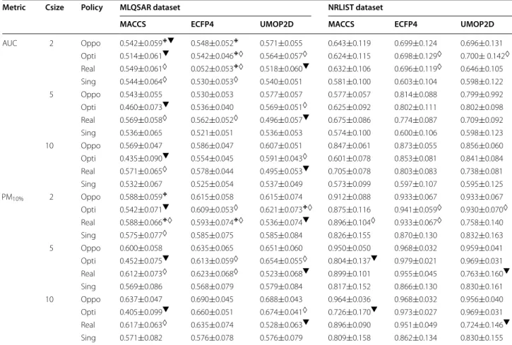
Table 3 Median AUC and PM values with their median absolute deviations

‘csize’ stands for consensus size. A ‘✠’ indicates that a distribution of peformance metric values is not significantly different from the one of the single policy (Kolmogorov–Smirnov test with p-value ≥0.05). A ‘◊’ indicates that a distribution of peformance metric values is not significantly different from the one of the

opportunist policy. A ‘▼’ indicates performance worse than the single policy

Metric Csize Policy MLQSAR dataset NRLIST dataset

MACCS ECFP4 UMOP2D MACCS ECFP4 UMOP2D

AUC 2 Oppo 0.542±0.059✠▼ 0.548±0.052✠ _0.571±0.055 _0.643±0.119 _0.699±0.124 _0.696±0.131 Opti 0.514±0.061▼ 0.542±0.046✠◊ 0.564±0.057◊ 0.624±0.115 0.698±0.129◊ 0.700± 0.142◊ Real 0.549±0.061◊ 0.052±0.053✠◊ 0.518±0.060▼ 0.632±0.106 0.696±0.119◊ 0.646±0.105 Sing 0.544±0.064◊ 0.530±0.053◊ 0.540±0.051 0.581±0.100 0.603±0.104 0.598±0.122 5 Oppo 0.543±0.055 0.530±0.053 0.577±0.057 0.577±0.057 0.814±0.088 0.799±0.992 Opti 0.460±0.073▼ 0.536±0.040 0.569±0.051◊ 0.625±0.092 0.802±0.111 0.802±0.098 Real 0.569±0.058◊ 0.562±0.052◊ 0.496±0.057▼ 0.675±0.086 0.774±0.087 0.709±0.092 Sing 0.536±0.065 0.521±0.051 0.536±0.053 0.574±0.100 0.600±0.106 0.598±0.123 10 Oppo 0.569±0.047 0.586±0.047 0.607±0.051 0.847±0.061 0.873±0.055 0.856±0.060 Opti 0.435±0.090▼ 0.554±0.045 0.591±0.043◊ 0.601±0.078 0.853±0.081 0.841±0.084 Real 0.571±0.065◊ 0.578±0.044 0.495±0.053▼ 0.705±0.078 0.803±0.083 0.738±0.081 Sing 0.532±0.067 0.525±0.054 0.537±0.049 0.573±0.099 0.597±0.107 0.595±0.125 PM10% 2 Oppo 0.588±0.059✠ 0.615±0.058 0.615±0.074 0.912±0.088 0.933±0.067 0.933±0.067 Opti 0.542±0.071▼ 0.609±0.053◊ 0.621±0.073✠◊ 0.875±0.116 0.941±0.059◊ 0.930±0.070◊ Real 0.588±0.066✠◊ 0.593±0.074✠◊ 0.536±0.074▼ 0.896±0.104◊ 0.933±0.067◊ 0.758±0.140 Sing 0.575±0.077◊ 0.585±0.075 0.585±0.084 0.826±0.155 0.870±0.130 0.832±0.163 5 Oppo 0.600±0.058 0.635±0.065 0.651±0.060 0.950±0.050 0.968±0.032 0.959±0.041 Opti 0.452±0.075▼ 0.613±0.059◊ 0.654±0.055◊ 0.804±0.137▼ 0.979±0.021 0.969±0.031 Real 0.612±0.073◊ 0.623±0.068◊ 0.523±0.068▼ 0.899±0.101 0.955±0.045 0.763±0.160▼ Sing 0.569±0.086 0.568±0.079 0.579±0.084 0.817±0.152 0.866±0.130 0.830±0.161 10 Oppo 0.637±0.047 0.690±0.045 0.688±0.043 0.964±0.036 0.968±0.032 0.956±0.040 Opti 0.405±0.099▼ 0.660±0.051 0.674±0.041◊ 0.726±0.170▼ 0.973±0.027 0.969±0.031 Real 0.617±0.063◊ 0.635±0.074 0.528±0.063▼ 0.896±0.090 0.951±0.049 0.724±0.146▼ Sing 0.571±0.082 0.576±0.078 0.576±0.079 0.809±0.158 0.862±0.134 0.830±0.155

-100 -80 -60 -40 -20 0 20 40 60

0 50 100 150 200 250

Median delta rank

Active molecule rank delta rank linear best fit

Fig. 8 Effect of applying potency scaling (knowledgeable policy) or not (realist policy) to build the consensus. The median change in rank is shown over 1000 experiments for all actives of the NRLIST PR-target (NRLIST target with the most active ligands) and MACCS fingerprints. Active molecules are ranked ordered from most to least potent (left to right)

Table 4 Cases where the knowledgeable consensus policy brings the most active molecules closer to the query com-pared to another policy

Experiment: all NRLIST targets, median change in rank over 500 experiments and ECFP4 fingerprint

Size Know verus real Know versus oppo

10 10/10 8/10

15 10/10 7/10

20 10/10 7/10

Table 5 Cases where the optimist query outperforms the opportunist one in CPU-bounded experiments

Size: consensus size; speedup: how many times the optimist consensus is faster at scoring than the opportunist consensus. Experiment: compute the accumulated curve of actives on MLQSAR (median curve over 10 experiments) and NRLIST (median curve over 50 experiments). The number of times where the optimist curve dominates the opportunist one is reported

Size Speedup MLQSAR NRLIST

5 1.46 6/9 9/10

10 2.05 7/9 8/10

(12)

Availability and requirements

Project Name: Consent

Project home page:

https://github.com/UnixJunkie/consent

Software archives:

http://meilerlab.org/software or

https://zenodo.org/record/1006728

Operating system: Linux, Mac OS X Programming language: OCaml

Other requirements: the OCaml Package Manager (OPAM), Open Babel, RDkit

Dataset:

https://data.mendeley.com/datasets/52hjy6vjwb/1

License: GPL

Any restrictions to use by non-academics: None Authors’ contributions

FB designed the study, wrote the software, ran experiments and prepared figures and tables. OV implemented MOLPRINT2D fingerprints in the BCL and computed the MOLPRINT2D fingerprints that were used early in the study. All authors have analyzed the results and participated in writing the manuscript. All authors read and approved the final manuscript.

Author details

1_{Department of Chemistry, Vanderbilt University, Nashville, TN, USA.}2 Divi-sion of System Cohort, Medical Institute of Bioregulation, Kyushu University, Fukuoka, Japan.

Acknowledgments

Work in the Meiler laboratory is supported through NIH (R01 GM080403, R01 GM099842) and NSF (CHE 1305874). FB is a JSPS international research fellow http://www.jsps.go.jp/english/. FB acknowledges the use of Marvin-View v17.1.3 and JKlustor v0.07 from ChemAxon’s JChem (2017) http://www. chemaxon.com.

Competing interests

The authors declare that they have no competing interests.

Consent for publication

Not applicable.

Ethics approval and consent to participate

Not applicable.

Publisher’s Note

Springer Nature remains neutral with regard to jurisdictional claims in pub-lished maps and institutional affiliations.

Received: 20 June 2017 Accepted: 20 November 2017

References

1. Lake BM, Salakhutdinov R, Tenenbaum JB (2015) Human-level con-cept learning through probabilistic program induction. Science 350(6266):1332–1338. https://doi.org/10.1126/science.aab3050

2. Altae-Tran H, Ramsundar B, Pappu AS, Pande V (2017) Low data drug discovery with one-shot learning. ACS Cent Sci 3(4):283–293. https://doi. org/10.1021/acscentsci.6b00367

3. Johnson MA, Maggiora GM (1990) Concepts and applications of molecu-lar simimolecu-larity. Wiley, New York ISBN 978-0-471-62175-1

4. Bender A, Glen RC (2004) Molecular similarity: a key technique in molecu-lar informatics. Org Biomol Chem 2:3204–3218. https://doi.org/10.1039/ B409813G

5. Willett P (2006) Similarity-based virtual screening using 2D finger-prints. Drug Discov Today 11(23):1046–1053. https://doi.org/10.1016/j. drudis.2006.10.005

6. Shemetulskis NE, Weininger D, Blankley CJ, Yang JJ, Humblet C (1996) Stigmata: an algorithm to determine structural commonalities in diverse datasets. J Chem Inf Comput Sci 36(4):862–871. https://doi.org/10.1021/ ci950169+

7. Singh SB, Sheridan RP, Fluder EM, Hull RD (2001) Mining the chemical quarry with joint chemical probes: an application of latent semantic structure indexing (LaSSI) and toposim (Dice) to chemical database min-ing. J Med Chem 44(10):1564–1575. https://doi.org/10.1021/jm000398+

8. Xue L, Stahura FL, Godden JW, Bajorath J (2001) Fingerprint scaling increases the probability of identifying molecules with similar activity in virtual screening calculations. J Chem Inf Comput Sci 41(3):746–753.

https://doi.org/10.1021/ci000311t

9. Hert J, Willett P, Wilton DJ, Acklin P, Azzaoui K, Jacoby E, Schuffenhauer A (2004) Comparison of fingerprint-based methods for virtual screening using multiple bioactive reference structures. J Chem Inf Comput Sci 44(3):1177–1185. https://doi.org/10.1021/ci034231b

0 10 20 30 40 50 60 70 80 90 100

0 20 40 60 80 100 120 140 160

Cumulated actives (molecule)

Molecule rank opti oppo

0 20 40 60 80 100 120 140

0 20k 40k 60k 80k 100k 120k 140k 160k 180k Molecule rank

opti oppo

(13)

10. Godden JW, Stahura FL, Bajorath J (2004) Pot-dmc: a virtual screening method for the identification of potent hits. J Med Chem 47(23):5608– 5611. https://doi.org/10.1021/jm049505g

11. Whittle M, Gillet VJ, Willett P, Loesel J (2006) Analysis of data fusion meth-ods in virtual screening: similarity and group fusion. J Chem Inf Modeling 46(6):2206–2219. https://doi.org/10.1021/ci0496144

12. Vogt I, Bajorath J (2007) Analysis of a high-throughput screening data set using potency-scaled molecular similarity algorithms. J Chem Inf Modeling 47(2):367–375. https://doi.org/10.1021/ci6005432

13. Wang Y, Bajorath J (2008) Bit silencing in fingerprints enables the deriva-tion of compound class-directed similarity metrics. J Chem Inf Modeling 48(9):1754–1759. https://doi.org/10.1021/ci8002045

14. Schultes S, Kooistra AJ, Vischer HF, Nijmeijer S, Haaksma EEJ, Leurs R, de Esch IJP, de Graaf C (2015) Combinatorial consensus scoring for ligand-based virtual fragment screening: a comparative case study for serotonin 5-HT3A, histamine H1, and histamine H4 receptors. J Chem Inf Modeling 55(5):1030–1044. https://doi.org/10.1021/ci500694c

15. Polishchuk PG, Madzhidov TI, Varnek A (2013) Estimation of the size of drug-like chemical space based on GDB-17 data. J Comput Aided Mol Des 27(8):675–679. https://doi.org/10.1007/s10822-013-9672-4

16. Sterling T, Irwin JJ (2015) Zinc 15—ligand discovery for everyone. J Chem Inf Modeling 55(11):2324–2337. https://doi.org/10.1021/acs.jcim.5b00559

17. Reymond J-L, Awale M (2012) Exploring chemical space for drug discovery using the chemical universe database. ACS Chem Neurosci 3(9):649–657. https://doi.org/10.1021/cn3000422

18. Ruddigkeit L, Blum LC, Reymond J-L (2013) Visualization and virtual screening of the chemical universe database GDB-17. J Chem Inf Mod-eling 53(1):56–65. https://doi.org/10.1021/ci300535x

19. Mysinger MM, Carchia M, Irwin JJ, Shoichet BK (2012) Directory of useful decoys, enhanced (DUD-E): better ligands and decoys for better benchmarking. J Med Chem 55(14):6582–6594. https://doi.org/10.1021/ jm300687e

20. Lagarde N, Ben Nasr N, Jérémie A, Guillemain H, Laville V, Labib T, Zagury J-F, Montes M (2014) Nrlist bdb, the manually curated nuclear receptors ligands and structures benchmarking database. J Med Chem 57(7):3117– 3125. https://doi.org/10.1021/jm500132p

21. Butkiewicz M, Lowe EW, Mueller R, Mendenhall JL, Teixeira PL, Weaver CD, Meiler J (2013) Benchmarking ligand-based virtual high-throughput screening with the pubchem database. Molecules 18(1):735–756. https:// doi.org/10.3390/molecules18010735

22. O’Boyle Noel, Banck Michael, James Craig, Morley Chris, Vandermeersch Tim, Hutchison Geoffrey (2011) Open Babel: an open chemical toolbox. J Cheminform 3(1):33. https://doi.org/10.1186/1758-2946-3-33

23. Tosco P, Stiefl N, Landrum G (2014) Bringing the MMFF force field to the RDKit: implementation and validation. J Cheminform 6(1):37. https://doi. org/10.1186/s13321-014-0037-3

24. Landrum G. RDKit: Open-source cheminformatics. http://www.rdkit.org

25. Bender A, Mussa HY, Glen RC, Reiling S (2004) Similarity searching of chemical databases using atom environment descriptors (MOLPRINT

2D): evaluation of performance. Journal of Chemical Information and Computer Sciences 44(5):1708–1718. https://doi.org/10.1021/ci0498719

26. Bender A, Mussa HY, Glen RC, Reiling S (2004) Molecular similarity search-ing ussearch-ing atom environments, information-based feature selection, and a naïve bayesian classifier. J Chem Inf Comput Sci 44(1):170–178. https:// doi.org/10.1021/ci034207y

27. Kothiwale S, Mendenhall JL, Meiler J (2015) Bcl::conf: small molecule conformational sampling using a knowledge based rotamer library. J Cheminform 7(1):47. https://doi.org/10.1186/s13321-015-0095-1

28. Sastry M, Lowrie JF, Dixon SL, Sherman W (2010) Large-scale systematic analysis of 2D fingerprint methods and parameters to improve virtual screening enrichments. J Chem Inf Modeling 50(5):771–784. https://doi. org/10.1021/ci100062n

29. Lopes JCD, dos Santos FM, Martins-José A, Augustyns K, De Winter H (2017) The power metric: a new statistically robust enrichment-type metric for virtual screening applications with early recovery capability. J Cheminform 9(1):7. https://doi.org/10.1186/s13321-016-0189-4

30. Leroy X, Doligez D, Frisch A, Garrigue J, Rémy D, Vouillon J (2016) The ocaml system release 4.04- documentation and user’s manual 31. Danelutto M, Cosmo RD (2012) A Minimal Disruption Skeleton

Experiment: Seamless Map and Reduce Embedding in OCaml. Pro-cedia Computer Science 9(0), 1837–1846. https://doi.org/10.1016/j. procs.2012.04.202. Proceedings of the International Conference on Computational Science, ICCS 2012

32. Berenger F, Coti C, Zhang KYJ (2010) PAR: a PARallel and distributed job crusher. Bioinformatics 26(22):2918–2919. https://doi.org/10.1093/ bioinformatics/btq542

33. Kerber A, Laue R, Meringer M, Rücker C (2007) Molecules in silico: a graph description of chemical reactions. J Chem Inf Modeling 47(3):805–817.

https://doi.org/10.1021/ci600470q

34. Hoksza D, Škoda P, Voršilák M, Svozil D (2014) Molpher: a software frame-work for systematic chemical space exploration. J Cheminform 6(1):7.

https://doi.org/10.1186/1758-2946-6-7

35. Naderi M, Alvin C, Ding Y, Mukhopadhyay S, Brylinski M (2016) A graph-based approach to construct target-focused libraries for virtual screening. J Cheminform 8(1):14. https://doi.org/10.1186/s13321-016-0126-6

36. Liu T, Naderi M, Alvin C, Mukhopadhyay S, Brylinski M (2017) Break down in order to build up: decomposing small molecules for fragment-based drug design with emolfrag. J Chem Inf Modeling 57(4):627–631. https:// doi.org/10.1021/acs.jcim.6b00596