Inferring multi-target QSAR models with taxonomy-based multi-task learning

R E S E A R C H A R T I C L E

Open Access

Inferring multi-target QSAR models with

taxonomy-based multi-task learning

Lars Rosenbaum

, Alexander Dörr

, Matthias R Bauer

, Frank M Boeckler

and Andreas Zell

Abstract

Background: A plethora of studies indicate that the development of multi-target drugs is beneficial for complex diseases like cancer. Accurate QSAR models for each of the desired targets assist the optimization of a lead candidate by the prediction of affinity profiles. Often, the targets of a multi-target drug are sufficiently similar such that, in principle, knowledge can be transferred between the QSAR models to improve the model accuracy. In this study, we present two different multi-task algorithms from the field of transfer learning that can exploit the similarity between several targets to transfer knowledge between the target specific QSAR models.

Results: We evaluated the two methods on simulated data and a data set of 112 human kinases assembled from the public database ChEMBL. The relatedness between the kinase targets was derived from the taxonomy of the humane kinome. The experiments show that multi-task learning increases the performance compared to training separate models on both types of data given a sufficient similarity between the tasks. On the kinase data, the best multi-task approach improved the mean squared error of the QSAR models of 58 kinase targets.

Conclusions: Multi-task learning is a valuable approach for inferring multi-target QSAR models for lead optimization. The application of multi-task learning is most beneficial if knowledge can be transferred from a similar task with a lot of in-domain knowledge to a task with little in-domain knowledge. Furthermore, the benefit increases with a decreasing overlap between the chemical space spanned by the tasks.

Keywords: Proteochemometrics, QSAR, Multi-target, Support vector machine, Kinome, Machine learning, Multi-task, Domain adaption

Background

Much has happened in the process of rational drug discov-ery in the last decades. The technology of next-generation sequencing [1] with its possibility to sequence genomes in an accelerating pace pushed the door open to a new set of targets approachable by existing and future drugs. Additionally, the methods of combinatorial chemistry [2] enable pharmaceutical chemists to generate large com-pound libraries by synthesizing more and more drug-like molecules. To process these enormous amounts of data, advances in the field of high-throughput screening com-plement the previously mentioned methods in a way that an increasing number of compounds can be screened

*Correspondence: [email protected]; [email protected]

†_{Contributed equally}

1Center for Bioinformatics (ZBIT), University of Tübingen, Sand 1, Tübingen 72076, Germany

Full list of author information is available at the end of the article

against desired biological targets with a decreasing finan-cial effort [3]. Regarding these facts and looking at the increased amount of R&D investments, one could argue that the drug discovery pipeline should be in full swing yielding a growing amount of approved drugs. Albeit, the number of novel drugs did not increase but rather, if any, stayed constant [4].

A joint starting point of many drug design approaches is an exhausting search for a drug-like molecule that binds with a high affinity to a desired biological tar-get. However, recent findings have shown that looking for such a high affinity binder for a specific receptor is not crowned with success in every case. Even if single-target drugs can evoke the pursued effect on their specific biological target, this does not necessarily apply to the whole organism [5,6]. For example the targets associated with the treatment of complex diseases like impairment of the CNS, cancer, metabolic disorders, or AIDS are diverse and several disease related mechanisms have to

be taken into account [7,8]. Targeting multiple proteins is required for these diseases because medication of the dis-eased state is intercepted by the way the proteins interact such that back-up circuits or fail-safe mechanisms take effect. These backup systems can be sufficiently dissim-ilar that they do not respond to a highly selective drug [8-11]. Hence, in cancer therapy, drugs with a single or few targets can be doomed to failure, since resistances are more easily to arise than if pressure is exerted on more targets [12].

In addition to new ways of treating diseases like cancer, the approach of multi-target drug design offers various advantages. Using a single molecule for different pathways in a chemotherapy increases its therapeutic effectiveness, and it is much easier to manage absorption and elimi-nation for one molecule than for several [13]. Compared to single-target drugs that bind with a high affinity to their target, multi-target drugs are considered low-affinity binders [6]. From this fact it follows that multi-target drugs are not subject to the high constraints for high-affinity binding and, furthermore, allow for targeting a greater number of proteins [8]. In some cases, like the operation of NMDA receptor antagonists, it is in fact desirable to bind with a lower affinity, since shutting this receptor completely down is impairing its normal func-tion [14,15]. There is also evidence that several small interventions to various targets, as achieved with multi-target drugs, can have a greater effect on the outcome than a strong single perturbation [6,16].

The multi-target drug design approach is a promis-ing way to complement the existpromis-ing spromis-ingle-target pro-cess and a plethora of studies address the problem of target prediction [17] and multi-target structure-activity models [18-20]. Ma et al. [18] evaluated support vector machine (SVM) classification models of several biologi-cal targets for common hits. Heikamp et al. [19] linearly combined independently derived SVM models by assign-ing a distinct weight to each model. Ajmani et al. [20] inferred models for three kinases with PLS regression methods and evaluated the models for common struc-tural requirements to inhibit the kinases. These studies show that multi-target drug prediction is a contempo-rary research topic in the field of drug design. Despite the positive results of the studies mentioned above, the considered models were still trained for each target separately.

Studies in the field of multi-task and transfer learn-ing suggested a promislearn-ing way to combine knowledge from problem-related tasks into a single SVM model. Schweikert et al. [21] argued that from the kinship of organism one can see analogous biochemical processes. Therefore, it is possible to transfer the knowledge of a bio-logical problem to another domain if both problems are sufficiently related to each other. This domain adaption

approach was successfully applied to the binding predic-tion of MHC class I molecules and splice site detecpredic-tion [22]. Looking beyond the lead identification process and with it the classification of molecules, support vector regression (SVR) can be utilized to reveal and address the specific affinity of molecules during the optimization of potential drugs. Developing a multi-target agent requires to monitor the affinity against a panel of similar targets. Thus, adapting multi-task classification to a regression setting should be beneficial for the lead optimization of multi-target drugs. Multi-target regression algorithms can compensate for a fewer amount of training instances avail-able for a problem by exploiting the knowledge of a similar problem.

The concept of taxonomy-based transfer learning is similar to the concept of overlapping ligand–target spaces in the field of proteochemometric modeling. A proteochemometric model is trained on instances that combine target descriptors with ligand descriptors. An overview of proteochemometrics can be found in a recent review by van Westen et al. [23]. In contrast to proteochemometric models, transfer learning algorithms infer target specific models solely on ligand descriptors, but force the models to be similar according to some target similarity or taxonomy.

In this paper, we present two different multi-task regres-sion algorithms based on the multi-task classifiers of Widmer et al. [22]. We demonstrate the effectiveness of the algorithms by inferring multi-target QSAR mod-els on a subset of the human kinome. The taxonomical relationship of the kinase targets should correlate with the relatedness of the QSAR problems on these targets. Hence, we derived the relatedness of the problems from the human kinome tree [24]. We compared our multi-task methods to SVM models that were independently trained for each target and an SVM model that assumed all targets to be identical. We evaluated the methods on simulated data sets, a data set with affinity data against a large frac-tion of the human kinome, and four smaller subsets of the aforementioned kinome data.

The results show that multi-target learning results in a considerable performance gain compared to the baseline methods if knowledge can be transferred from a target with a lot of data to a similar target with little domain knowledge.

Methods

Standard support vector regression (SVR)

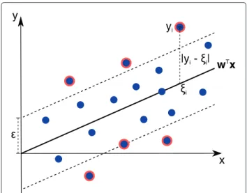
A single-target QSAR problem comprises a set ofllabeled fingerprints {(xi,yi),i = 1,. . .,l}, wherexi ∈ Rn is a fingerprint of a compound andyi ∈ Ris a pIC50 or pKi value. Given such a QSAR data set the standard support vector regression (SVR) solves the constrained optimiza-tion problem shown in Equaoptimiza-tion 1, which is also known as primal problem. A visualization of the problem’s variables is presented in Figure 1.

min

w,ξ

1 2||w||

2_+Cl

i=1

l(ξi,yi)

s.t. ξ_i=wTxi

(1)

In Equation 1, the term ||w||2 _{regularizes the model} complexity,C > 0 is a user-defined parameter and the -insensitive loss functionlis defined as follows.

l(ξi,yi)=

max(|ξ_i−yi| −, 0) or

max(|ξ_i−yi| −, 0)2 (2)

The functionl ensures that the loss is zero if|wTxi−

yi| = |ξi−yi| ≤, which means that the actual target value yilies within an-insensitive tube aroundwTx. Equation 2 is commonly known as L1and L2SVR loss, respectively. In this study, we use the mean squared error (MSE) as error function, which is directly modeled by the L2loss. Hence, the equations throughout the paper assume that L2 loss is applied.

x

y

i

w

_x

y

|y

-

|

Figure 1Support vector regression (SVR).Illustration of an SVR regression function represented bywT_{x. The-insensitive tube} around the function is indicated by a gray tube.ξi=wTxiis the predicted target value ofxiandyirepresents the actual target value. Support vectors are indicated by a red border.

The dual problemfD(β)of L2loss SVR is presented in Equation 3, where Qij = xiTxj is the so called kernel matrix.

min

β fD(β)=

min β

1 2β

T_Qβ+l

i=1

|βi| −yiβi+ 1 4Cβ

2 i

₍₃₎

The data points, for whichβ_i = 0, are called support vectors. A data point is a support vector if and only if its actual target value yi is on the boundary or outside the -insensitive tube around the predicted valuewTxi. The larger the value of, the sparser the resulting SVR model, but the less precise the model needs to approximate the target values yi. For the derivation of the dual problem and a more detailed introduction to SVR theory, we refer to [25,26].

The dual problem (3) can be rapidly solved with the large-scale learning library LIBLINEAR [27]. The library uses a dedicated solver [26], which allows for training an SVR model with several hundred thousands of instances. However, the library is limited to the linear case, which means that the dot product kernel has to be used.

Generally, the dot product kernel results in larger simi-larity values with an increasing compound or fingerprint size. Hence, we normalize each fingerprint before train-ing, such that xi = 1. This normalization in combi-nation with the dot product kernel is equal to using the cosine kernel as shown in Equation 4.

kcos(xi,xj)= xi

T_xj

xixj (4)

The similarity values of the cosine kernel are normal-ized to [0, 1] and are independent of the fingerprint size. As a result, the cosine kernel generally performs better for chemical fingerprints than using the dot product kernel without normalization.

Multi-task learning

A multi-target QSAR data set with T different targets comprises a set of triples{(xi,yi,ti),i = 1,. . .,l}, where xi andyi are defined as for a single-target QSAR prob-lem, andti ∈ {1,. . .,T}indicates to which target protein the triple belongs to. For multi-target QSAR, inferring the QSAR model for a certain targett can be regarded as a separate learning task.

The goal of multi-task learning is to learn a set of func-tionsfT such thatfti(xi) ≈ yiand the setfT generalizes

of a well known domainsis transferred to a similar, less known domaint. By transferring knowledge, the resulting functionftshould generalize better on unseen data. Con-sequently, transfer learning should be most profitable if a learning task with very few training instances is similar to a learning task with many training instances.

The knowledge transfer is commonly achieved by forc-ing the functions fs and ft to be similar if the domains s and t are similar. For linear SVR models, a function ft(x)= wtTxis completely determined by its weight vec-torwt. The weightsw1,. . .,wTare forced to be similar by changing the SVR primal (1) to Equation 5.

min

w1,...,wT,ξ

1 2

T

t=1

||wt||2+J(w1,. . .,wT)

+C l

i=1

l(ξi,yi)

s.t. ξ_i=wtiTxi

(5)

The terms||wt||2control the task specific model com-plexity, like for standard SVR. The functionJ(w1,. . .,wT)

represents an additional regularization term that facili-tates the similarity of the weight vectors of similar tasks. The type of multi-task learning algorithm is determined by a specific choice of the regularizer J(w1,. . .,wT)

[28-31]. An example on how multi-task learning transfers knowledge between tasks is depicted in Figure 2.

x y

w1x

J(w1, ... ,wT)

unkown data for task 1 task 1

task 2 wT2x T

Figure 2Knowledge transfer in multi-task learning.Illustration of a knowledge transfer from task 2, which comprises a lot of training data (green), to a similar task 1, which contains little training data (blue). The-insensitive tubes around the regression functionsw1Tx andw2Txare colored gray. The regularizerJ(w1,. . .,wT)forces the model of task 1 (w1) to be more similar to the model of task 2 (w2). A modelw1that is more similar tow2predicts the unknown data (red) better, which results in a better generalization of the model.

Given an unseen data point x, the target value yfor a specific task t can be obtained by ft as shown in Equation 6.

y=ft(x)=wtTx (6)

A task specific bias termbtcan be included in the train-ing and in the decision function by addtrain-ing the bias to the weight vector as shown in Equation 7.

˙ wt=

wt

bt

,x˙ =

x 1

(7)

Including the bias term into the weight vector results in a regularization of the bias, which can be a problem if a larger bias is required. Furthermore, the similarity between the tasks is facilitated by regularizing the task specific weights. Given two similar tasks with consider-ably different bias terms, the regularization can result in mainly forcing the bias to be similar and not the fea-ture specific weights. To avoid this problem, we centered the target values y directly before the optimization and used the offset as bias. For high dimensional data, such as sparse chemical fingerprints, a bias term as shown in Equation 7 is often not required [26,27]. While we did not include regularized bias terms in our experiments because of the aforementioned reason, it can be profitable for GRMT if the average target values of the tasks differ substantially.

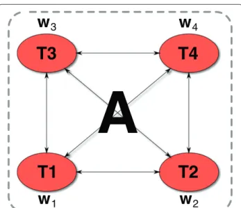
Graph-regularized multi-task (GRMT) SVR

Evgeniou et al. introduced an approach that uses graph-based regularization [29,30]. In their approach, each task corresponds to a node in a graph and the similarity between the tasks is encoded by weighted edges sum-marized in an adjacency matrix A, where Ast ≥ 0 (see Figure 3). The resulting regularizationJ(w1,. . .,wT)

is the sum of similarity weighted distances between the weight vectors as presented in Equation 8. Using the graph LaplacianL=D−Aof a given adjacency matrixA, where Dst= δst kAkt, the regularizer can also be expressed as shown in Equation 9.

J(w1,. . .,wT)= 1

4 T

s=1 T

t=1

Ast||ws−wt||2 (8)

= 1 2

T

s=1 T

t=1

LstwsTwt (9)

T1

T2

T3

T4

A

w

w

w

w

Figure 3Graph-regularized multi-task (GRMT) SVR training.The example shows four tasks, represented by four nodes of a graph, and their corresponding weight vectorsw1,. . .,w4. The tasks are related by a real-valued adjacency matrixA. GRMT trains the task specific modelsw1,. . .,w4in a single step, indicated by a dashed box, using the instances of all tasks.

The primal GRMT SVR optimization problem is obtained by combining Equations 5 and 9, which results in the following problem.

min

w1,...,wT,ξ

1 2

T

t=1

||wt||2+ 1

2 T

s=1 T

t=1

LstwsTwt

+C l

i=1

l(ξi,yi)

s.t. ξ_i=wtiTxi

(10)

Widmer et al. [32] proposed an alternative formula-tion of the primal for GRMT classificaformula-tion, which com-bines the task specific weights w1,. . .,wT into a single weight vectorw. This alternative formulation uses the so-called “block vector view”. Furthermore, they proposed a new dualization technique, which allows for the deriva-tion of a dual problem that can be optimized with an adapted version of the LIBLINEAR solver [26,27]. With the LIBLINEAR solver, the efficient training of large-scale graph-regularized multi-task problems becomes feasible.

For formulating the GRMT SVR primal problem similar to the classification formulation of Widmer et al., we first introduce the “block vector view”. The “block vector view” can be defined as shown in Equations 11 and 12, whereIn is then-dimensional identity matrix andL ∈ RT×T. The

injective functionψ :Rn→RnTmaps a fingerprintxito a vector that is zero, except for theti-th block.

block(L):=

⎛ ⎜ ⎝

L11In · · · L1TIn ..

. . .. ... LT1In · · · LTTIn

⎞ ⎟

⎠ (11)

ψ(xi):=(0,. . ., 0,xiT, 0,. . ., 0)T ↑

ti−th block

(12)

With the “block vector view”, the primal optimization problem for GRMT SVR (10) can be reformulated as follows.

min

w,ξ

1 2w

T_block(I

T+L)w+C l

i=1

l(ξi,yi)

s.t. ξ_i=wTψ(xi)

(13)

The dual formulation of the primal (13) can be derived with the dualization technique of Widmer et al. Details on the derivation of the GRMT SVR dual can be found in Additional file 1. The dual GRMT problem can be stated as follows.

min β

1 2

l

i=1

βiψ(xi)

2

block(M)

+l i=1

|βi| −βiyi+ 1 4Cβ

2 i

where M:=(IT+L)−1 and x2_B:=xTBx

(14)

Similar to GRMT classification [32], the dual problem (14) can be solved using an adapted version of the LIBLIN-EAR solver [26,27]. Details on the adaption of the solver can be found in Additional file 1. With the adapted LIB-LINEAR solver, training a GRMT regression problem with more than 20,000 instances and over 100 tasks becomes feasible.

Top-down multi-task (TDMT) SVR

If the learning tasks or in our case protein targets are related by some taxonomy T, the hierarchical structure of T can be exploited to subsequently train more spe-cialized models. We assume that the longer the common evolutionary history of two targets, the more similar the structure of the proteins, and the more beneficial it should be to share information between the learning tasks. In such a taxonomy, leaves correspond to learning tasks that are related by the inner nodes.

models while descending the taxonomy. The successive specialization is achieved by minimizing the training error with respect to the training instances of the current sub-tree, while maintaining similarity to the ancestor by an additional regularization term (see Figure 4). The primal optimization problem at a certain node of the taxonomy can be formulated as follows.

min

w

1−B 2 ||w||

2₊B 2||w−w

∗

p||2+C

i∈S

l(ξi,yi)

s.t. ξ_i=wTxi

(15)

In Equation 15, the setScontains the training instances i, for which the task ti is a leaf of the current sub-tree. The weightw∗_pis the optimal weight of the parent’s SVR model, which is fixed during the optimization of the current model. The parameterB∈[ 0, 1] controls the trade-off between the margin of the current model and the similarity to the parents modelw∗_p. SettingB=0 cor-responds to training a model that is independent of its ancestor, whereas settingB=1 represents a model that is maximally dependent on its ancestor.

The primal (15) can be reformulated to the following problem.

min

w

1 2||w||

2_−BwT_w∗

p+C

i∈S

l(ξi,yi)

s.t. ξ_i=wTxi

(16)

The alternative formulation (16) shows that the TDMT optimization problem only has an additional linear term compared to the standard SVR primal (1). Equation 17 denotes the dual optimization problem, which, limited to

the setS, is also identical to the standard SVR dualfD(β) of Equation 3 except for an additional linear term.

min

β fD(β)−

i∈S

βiB w∗pTxi pi

(17)

The linear termspi can be pre-computed before opti-mization and passed to the solver as additional linear term. Hence, the optimization problem (17) can be effi-ciently solved with any existing SVR solver by extending the solver to handle custom linear termspi. We extended the Java port of LIBLINEAR to handle additional lin-ear terms. As a result, the optimization of a top-down model is as fast as training an independent model. How-ever, a top-down model for each node of the taxonomyT has to be calculated, which is more time consuming than inferring models for the leaves only.

For the prediction of an unseen data pointx, we need to take into account the weight of the model and the weight of the parent as formulated in Equation 18.

f(x)=(w+w∗_p)Tx (18)

Task similarity parameters

Besides the standard SVR parametersC and, the task similarity is an essential parameter for multi-task regres-sion. For GRMT the task similarity is encoded in the adjacency matrix A, whereas for TDMT the similarity is encoded in the parameter B. In principle, each edge e of the taxonomy can have a weight or distance, which results in a parameter Be for each node model. Hence, the similarity information of the taxonomy can be used as parameters. For TDMT, the weights of the taxonomy are scaled to [ 0, 1] and the parametersBeare set to the scaled weights. A completely weighted taxonomy can be trans-formed to a distance matrix, where the distance of two taxa is the weight of the shortest path between the two taxa. To obtain a similarity matrixAthe distance matrix is

a

b

c

normalized to [ 0, 1] and the distancesdare transformed to a similaritys=1−d.

A simple approach to learn the task similarity for TDMT is based on cross-validation [22]. However, searching the bestBeof all nodes in a joint grid search is too expensive. A feasible approach is to do a local grid search for the best Beat each node, which can be interpreted as a heuristic that limits the parameter search space based on the given taxonomy.

A problem for multi-task approaches can be negative transfer [31]. Negative transfer is knowledge transfer that results in a worse performance compared to a regres-sion model without knowledge transfer. For the TDMT approach, it is possible to prevent negative transfer by adding the parameterB=0 to the grid search at the leaves to allow for an independent model, even if the parameters are given by the weighted edges of a taxonomy.

Baseline methods

To compare the benefit of knowledge transfer of both TDMT and GRMT, we also evaluated the two baseline methods tSVM and 1SVM. The tSVM represents the usual approach whereby each of the T tasks stands for a single kinase and T independent standard regression SVMs are trained. So each of the resulting T models reflects solely the information provided by the corre-sponding kinase. For TDMT, thetSVM is equivalent to setting B = 0 for all leaves. GRMT with the similarity A=IT, whereIT is theT-dimensional identity matrix, is also equivalent totSVM, with the difference that the same SVR parameterCis used for each of the separate models. Compared to thetSVM, the 1SVM represents the oppo-site extreme, where one model is trained on the whole kinome with the implication that all problems and all kinases are assumed to be identical. This implication is equivalent to training the root of a TDMT (see Figure 4a). SettingAst = 1.0 for alli,jfor GRMT results in a model, which is similar to 1SVM. Thus, TDMT and GRMT can be configured to be similar to both extremes and the task similarity allows for specifying from which tasks and to what extent knowledge is communicated.

Molecular encoding

To generate the molecular fingerprints for SVR, we used the Java library jCompoundMapper developed by Hinselmann et al. [33]. With this library the extended-connectivity fingerprints (ECFP) were calculated for every compound used for training and testing. ECFPs [34] are common circular topological fingerprints that are fre-quently used for automatic comparison of molecules. As additional preferences we used a radius of 3 bonds (ECFP_6) and a hash space of size 220_{bits for the} result-ing hashed fresult-ingerprints. The reduction of the hash space

from the standard 232bits of the ECFP to 220bits resulted in≤ 0.5% and 4.2% colliding bits for the kinase subsets and the whole kinome data, respectively. Details on the hashing procedure can be found in the documentation of jCompoundMapper [33]. Additionally, we removed fea-tures that occur in more than 90% of the compounds for the whole kinome data.

A quality that speaks for the use of ECFPs is their interpretability. After training an SVM model, mappings between the hashed fingerprints and their correspond-ing substructure in the molecules of the traincorrespond-ing set can be established. This mapping enables a user to assign an importance to each atom and bond in a given com-pound. The importance can then be visualized with a heat map coloring [35]. For QSAR models, the weight of a substructure directly correlates with its activity contribution [36].

Experimental

In this section, we first describe the data sets used for eval-uation, which includes simulated as well as chemical data. Then, we present the parameters of the algorithms and the grid search ranges used for the experiments. Finally, we describe the statistical tests that were used to measure the significance of the differences between the algorithms.

Simulated data

To analyze the behavior of multi-task regression in a con-trolled setting, we simulated data, varying the number of instances, the number of tasks, and the dimensionality. We adapted the simulation design of other researchers for the evaluation of multi-task classification [29,37]. Using a real-valued label instead of a class label, the design can be adopted to multi-task regression.

Each data point comprisesDdifferent attributes, where Dcontrols the dimensionality of the data. Each attribute can adopt 6 different values, which represent an influence on the target value from very negative to very positive. The choice of each attribute is encoded by a 6-dimensional binary vector, e.g. (100000) for very positive and (000001) for very low. Thus, each data pointxiis a 6×D dimen-sional binary vector. The simulated data of [29,37] used only 4 attribute values, but we decided to increase the number of attribute values to better reflect the complexity of chemical fingerprints.

We generated models forT different tasks, each com-prising N different training instances. The N training instances were sampled separately for each task. A model is encoded by a 6×Ddimensional weight vector, where the weights were sampled attribute wise. Hence, the weight of a tasktis a vector

where (wj1,. . .,wj6) are the weights corresponding to thej-th attribute. The weights of an attribute were ran-domly sampled from a Gaussian with mean

−β,−2

3β,− 1 3β,

1 3β,

2 3β,β

.

The target valuesyof the tasks were calculated using the standard multi-task prediction function (6), which means that the target values do not contain label noise.

The parameter β controls the noise in the data. The lower the value ofβ, the higher the noise in the data. We used β = 3, which corresponds to a low noise in the data [29,37]. The similarity between the tasks can be con-trolled by varying the varianceσ2of the aforementioned Gaussian, where higher values ofσ2represent a lower task similarity. We used σ2 = 3β to model a low task simi-larity andσ2 = 0.5β for modeling a high task similarity, again like in [29,37]. To give an idea on howσ2influences the task similarity, we calculated the cosine similarity (4) between the tasks forN = 100,T = 10, andD = 10. A low task similarity resulted in a pairwise similarity of 0.32±0.12 between the tasks, whereas a high task sim-ilarity induced a pairwise simsim-ilarity of 0.75±0.05. This similarity was reflected by a Pearson correlation between the target values of 0.43±0.14 and 0.82±0.05 for low and high task similarity, respectively.

Summarized, the toy data can be varied in the dimen-sion D, the number of tasks T, the number of training instances per taskN, and the similarity between the tasks σ2_=sβ.

We calculated the task similarity for the multi-task algorithms from the weight vectors of the tasks. As tax-onomy we used a tree with a root node, representing the mean of the Gaussians, directly connected to the T tasks. As edge weights, we used the cosine similarity between the task models and the root node model, which uses the mean of the Gaussians as attribute weights. For the GRMT approach, we directly calculated the cosine similarity between the weight vectors of the task models.

Chemical data

For evaluating the multi-task algorithms on chemical data, we assembled a data set based on the ChEMBL database [38] with compounds against a large num-ber of human protein kinase targets. We searched the ChEMBL database for the protein kinases of a previ-ous study by Karaman et al., which comprises about 55% of the human kinome [39]. Karaman et al. examined the multi-kinase activity of several kinase inhibitors to assess the biological implications of their administration. The total amount of 317 kinases included 27 disease-relevant mutant variants. Of the remaining 290 distinct human protein kinases their equivalent representation in ChEMBL was identified, which resulted in 278 kinases.

MYLK could not be matched, because ChEMBL only con-tains MLCK which is a synonym for MYLK according to UniProt [40]. The six kinases RPS6KA1 to RPS6KA6 account for 11 kinases altogether, because they are partly subdivided into N-terminal and C-terminal domain. Since ChEMBL handles this division on a lower level of the database in the description of the assays, these 11 kinases were also omitted. In general, kinase inhibitors can be classified into various types according to their binding mode, e.g. ATP-competitive and non-ATP-competitive [41,42]. These diverse types bind different locations on a kinase and therefore differ chemically from each other. Hence, different types of kinase inhibitors should be dis-tinguished during experiments. However, it was not pos-sible to obtain the membership of each kinase inhibitor in an automated fashion. As a result, different types of kinase inhibitors were merged.

On the basis of the 278 matched kinases all compounds were gathered for each target. Similar to the study of Hu et al. [43], all compounds had to fulfill certain criteria to be in the final data set. The first criterion was a cer-tain ChEMBL confidence score. The ChEMBL confidence score of a compound states the confidence that the respec-tive compound was assigned to the correct target with respect to the assay used. The highest score a compound can achieve is the value 9. Hu et al. selected compounds with a confidence score of 9 and omitted every other com-pound. We also allowed compounds with a score of 8 because selecting compounds with only the highest score resulted in too many data sets with an infeasible size to perform two-deep cross-validation. Additionally, the selection was restricted to molecules for which an assay type binding (B) is declared. We further excluded entries mapped to a mutant variant of a kinase, e.g. EGFR(L858R). Since the binding pockets of mutants have different amino acids available, the binding properties of compounds may differ. Therefore, only compounds mapped to the wild type were included. Like Hu et al., the final criterion for the selection was a reasonably high pIC50 value. The pIC50 value of a compound had to be at least 5.00. A pIC50 value of ≤ 5.00 is equal to an IC50 value of ≥ 10.0μm and represents a weakly active or inactive com-pound. Furthermore, the pIC50 or IC50 value had to be determined exactly, which excludes activity values given as relation like e.g.< 50nM or> 50nM. All IC50 values were converted to pIC50 values during the filtering pro-cess. Compounds with multiple pIC50 that differed more than 1 log unit where rejected to obtain a higher data precision. If this was not the case, the geometric means over all pIC50 values for the respective compounds were calculated.

Molecular Weight≤900; -7≤AlogP≤9; Hydrogen Bond Acceptors≤18; Hydrogen Bond Donors≤18; Number of Rotatable Bonds≤18. Additionally, structures containing non-organic atoms were discarded as well.

Due to the viability of a cross-validation, we addition-ally excluded 166 protein kinases, which had less than 15 compounds mapped to them. We also found 10 groups of duplicate structures with 3 compounds each, whereby 2 groups belonged to PTK2B and 8 groups to MAPK14. Since these molecules appertained to one specific kinase only, we mapped the ChEMBL ID of two structures to the third for each group. After all filtering steps we obtained 23000 compounds in total.

To reflect the experiments with the simulated data, we generated additional smaller data sets with the prerequi-site that there have to be at least three kinases for every data set with an overlap of at least 85 molecules. To be more precise there has to be a pIC50 value for each of the selected kinases. As a result of these constraints, we got the four smaller data sets shown in Table 1. TK/PI3 depicts the tyrosine kinase (TK) family consisting of members from the SRC and ABl subfamily and the kinase PIK3CA of the more distant PI3/PI4-kinase family. The data of this subset comes from a study for dual inhibitors of tyrosine and phosphoinositide kinases [44]. MAPK is composed of members from the MAP kinase subfamily, also known as c-Jun N-terminal kinases, which belong to the CMGC Ser/Thr protein kinase family. The majority of the data of this subset (131 compounds) stems from 6 different studies (see ChEMBL for details), where 4 studies were conducted by the same laboratory. PIM consists of mem-bers from the PIM subfamily of the CAMK protein kinase family. Half of the data stems from one study, the major-ity of the remaining data points from 4 different studies. PRKC contains three members of the AGCs PKC subfam-ily. The data of this subset stems from many different small studies.

Like for the simulated data, we estimated the similarity between the different tasks by calculating the correlation between the actual target values of the tasks. However, we used the Spearman coefficient instead of the Pearson cor-relation because the pIC50 values cannot be assumed to be normally distributed. For the TK/PI3, MAPK, PIM, and

Table 1 Kinase subsets

Identifier Members Size Cluster sizes

TK/PI3 HCK, PIK3CA, SRC, ABL1 123 18, 20, 39, 22, 19, 5

MAPK MAPK8, MAPK9, MAPK10 142 32, 24, 15, 28, 21, 22

PIM PIM1, PIM2, PIM3, 91 14, 10, 16, 17, 11, 23

PRKC PRKCD, PRKCE, PRKCH 99 12, 10 , 7, 18, 35, 16

Every compound of a subset has a pIC50 value for each kinase of the subset. The chemotype clusters were calculated with a 6-median clustering on the Tanimoto distance matrix.

PRKC subsets we obtained Spearman correlations of 0.85-0.92, 0.67-0.85, 0.42-0.75, and 0.35-0.64, respectively. It should be noted that measuring the task similarity with a correlation measure does not capture potential differences between the average pIC50 values.

In order to evaluate the performance of the methods with respect to chemotypes, we generated a clustering on the basis of the chemical similarity between the molecules of each subset. We used a matrix with distance values based on the Tanimoto similarity and ak-medians clus-tering. On the basis of the within-cluster sum of squares we determined a suitable value of 6 fork. As a result, we calculated six clusters for each subset.

At last, the Standardizer was used for each data set to canonicalize and transform every molecule struc-ture, JChem 5.12.0, 2013, ChemAxon [45] (http://www. chemaxon.com). On the basis of the guidelines by Fourches et al. [46] we used the following configuration: remove small fragments, neutralize, tautomerize, aroma-tize, and add explicit hydrogens. Details on the chemical data and the assigned clusters are provided in Additional file 2.

Human kinome tree

To assess the relationships between the kinases used in our experiments, a Newick tree was generated. As a basis for this tree we used the binary dendrogram that was derived from the work of Manning et al. [24]. They built a kinome taxonomy based on the sequence similarities between the kinase domains. Each subfamily is divided in a binary fashion such that each node has two children at maximum. We also extracted the evolutionary distances of the kinases from the website http://kinase.com/human/ kinome/. The content of these pages supports the pub-lished work of Manning et al. In addition to the given tree, the two atypical protein kinases RIOK1 and PIK3CA con-tained in our data set were directly attached to the root. As for the distances, a maximum value of 1 was chosen to reflect their low sequence similarity to all other kinases in the data set.

Parameter settings

The task similarity for the chemical data was derived from the human kinome tree. The branch lengths of the tree were all in the range [0, 1], as were the pairwise task distances derived from the tree, except for the two atypi-cal kinases RIO1 and PIK3CA, which were added with a branch length of 1.0. Hence, no scaling to [0, 1] was nec-essary for both TDMT and GRMT. The similarity of the atypical kinases to all other kinases was set to 0.0 for the GRMT algorithm.

of two recent binding assays [47,48]. The IC50 values showed a relative deviation of≈ 25%. A relative devia-tion of 25% amounts to a deviadevia-tion in the pIC50 values of ≈ 0.1. Hence, we chose = 0.1 as parameter value for the regression SVM. A grid search for an optimal can improve the performance of the algorithms. However, preliminary experiments did not yield substantial differ-ences compared to = 0.1 and we decided to stick with models with less parameters.

Recent publications [49,50] on the uncertainty in het-erogeneous data such as ChEMBL showed that the error is usually higher than the 0.1 log units estimated in this study. The results of the studies show that the mean unsigned error is 0.44 log units for Ki data and 0.55 log units for IC50 data. These values might prove useful for estimatingin future studies.

The parameters B and C were determined by a grid search. For all experiments and algorithms, except GRMT on the kinome data, we used log₂(C) ∈ {−5,−3,. . ., 7}. For a large number of tasks GRMT often chose larger values forCbecause there are many weight vector com-binations compared to the loss term. For GRMT on the kinome data we searched log₂(C) ∈ {2, 4,. . ., 8}. The grid search for the parameter B of TDMT used B ∈

{0, 0.1, 0.25, 0.5, 0.75, 0.9, 1.0}.

Statistical analysis

In this study, the performance of an algorithm was eval-uated on several random data set splits for the kinase subsets and on several cross-validation folds for the whole kinome data. All algorithms use the same training and test splits, which means that the performance values of two algorithms on a data set split can be paired. Further-more, the performance values cannot be assumed to be normally distributed. Consequently, we used a two-sided Wilcoxon signed-rank test to decide if the performance of two algorithms differs significantly on a certain target. The significance level was set toα=0.05 for all tests.

On the kinase subsets, we compared multiple algo-rithms on a given target with each other for significant dif-ferences. Thus, we corrected thep-values of the Wilcoxon tests with Holm’s method [51] to control the family-wise error. On the whole kinome data, we compared a multi-task algorithm to a baseline method on all 112 kinase targets and recorded the number of significant differ-ences. Correcting thep-values of the Wilcoxon test with the Benjamini and Hochberg correction [52] ensures a false discovery rate of 5% in the number of significant differences.

Results and discussion

In this section we present the results of the five app-roachestSVM, 1SVM, TDMTgs, TDMTtax, and GRMT on the simulated data as well as the chemical data. The

chemical data can be divided into the kinase subsets and the kinome data. The TDMTgs and TDMTtax represent the TDMT algorithm, where the parameterBis defined by a grid search and by the taxonomy edge weights, respec-tively. All presented MSE performances were determined on external test data, which was not included for the training of the algorithms or the model selection.

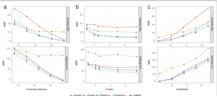
Simulated data

We simulated data varying the simulation parameters to capture the influence of the training set sizeN, the num-ber of tasksT, the dimensionalityD, and the task similarity on the performance of the five algorithms. We tested the following parameter ranges: For the training set sizeNwe usedN∈ {15, 30, 45, 60, 75}, for the number of tasksTwe choseT ∈ {2, 4, 5, 10, 15}, and the number of attributesD was set toD∈ {6, 10, 14, 18, 22}. For each parameter setup, we generated 10 random data sets for training and testing. The generation of 10 different splits should avoid a valida-tion bias induced by the random splitting procedure. Each test set contained 25 randomly generated test instances for each task with the same number of attributes as the training instances. Given a different number of training instancesN, the test set stayed the same. The parameters of the algorithms were searched with a 3-fold inner cross-validation on the training set. We employed a 3-fold inner cross-validation for the model selection to ensure a test set size of≥5.

0 20 40 60

High Similar

ity

20 40 60

MSE

0 20 40 60

High Similarity

4 8 12

MSE

MSE

0 50 100 150

Low Similarity

4 8 12

# tasks

0 50 100 150

Low Similarity

20 40 60

# training instances

MSE

0 20 40 60 80

High Similarity

10 15 20

MSE

a

0 50 100 150 200

Low Similarity

10 15 20

# attributes

MSE

b

c

tSVM 1SVM TDMTtax TDMTgs GRMT

Figure 5Performance on simulated data.Average mean squared error (MSE) while varying (a) the training set sizeN, (b) the number of tasksT, and (c) the number of attributesD. Varying a certain parameter, we kept the other parameters fixed toN₌45,T₌5, andD₌14. The average MSE was calculated from the performance on the 10 randomly generated test data sets for each parameter setup. The upper graphs show results for high task similarity, the lower graphs for low task similarity.

Another important factor is how much additional input space is covered by the similar tasks. The multi-task approaches benefit when the tasks cover a diverging por-tion of the input space. If a taskscovers a different region of the input space than a similar task t, knowledge can be transferred between the tasks, such that both tasks generalize well on both regions of the input space. To eval-uate the influence of the additional input space coverage gained from similar tasks, we generated the same training instances for all tasks. Still, the target valuesywere dif-ferent for the tasks because of the task specific models. For this simulation setup, all tasks cover the same portion of the input space and no additional coverage is achieved by transferring knowledge between the tasks. Given this setup, the multi task approaches performed equal to the tSVM because it is better to use the target values of the actual task than transferring knowledge from the target value of a similar task.

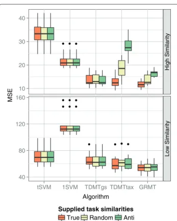
Further important aspects are the influence of the task similarities supplied to the algorithms and the prevention of negative transfer. To test the impact of the supplied task similarities on the performance of TDMTtax and GRMT, we compared the true task similarities with anti corre-lated similarities and random similarities. The true task similarities were estimated with the cosine similaritykcos between the weight vectors of the models, the anti cor-related task similarities were calculated by 1−kcos, and the random task similarities were set to uniformly dis-tributed random numbers from the interval [0, 1]. The similarity of a task to itself was fixed to 1.0 for all setups.

The results are depicted in Figure 6. The 1SVM, thetSVM, and TDMTgs do not use the supplied task similarity or determine the similarity in a grid search. Consequently, the supplied similarities did not considerably influence the performance of the algorithms. We conjecture that the small performance differences for TDMTgs are due to the randomization within the LIBLINEAR solver. For a low similarity between the simulated tasks the supplied simi-larity had only marginal influence, even if the algorithms were provided with anti correlated task similarities. For a high similarity between the tasks, GRMT was less prone to changes in the supplied task similarities than TDMT-tax. Provided with anti correlated task similarities, the performance of TDMTtax and GRMT decreased by 120% and 40%, respectively. Thus, the task similarity is a sen-sible parameter for TDMTtax, whereas GRMT is more robust against changes in the supplied task similarities. It should be stated that the simulated data employed a very simple taxonomy because all tasks were direct chil-dren of the root task. Earlier studies showed, that the gain of top-down learning increases with an increasing depth of the hierarchy [53]. Hence, the simple taxonomy of the simulated data might benefit GRMT.

10 20 30 40

40 80 120 160

High Similarity

Low Similarity

tSVM 1SVM TDMTgs TDMTtax GRMT

Algorithm

MSE

Supplied task similarities

True Random Anti

Figure 6Performance varying the supplied similarities.Mean squared error (MSE) while varying the supplied similarities. Each boxplot visualizes the performance on the 10 randomly generated test splits. True stands for correct task similarities given bykcos, Anti for anti correlated similarities given by 1₋kcos, and Random for random similarities. The upper graph shows results for a high task similarity between the simulated tasks, the lower graph for a low similarity.

taxonomies with incorrect task similarities. Hence, nega-tive transfer should not prevented for TDMTtax.

Kinase subsets

We evaluated the five algorithms on the kinase subsets. Each subset contains only compounds that are annotated with pIC50 labels for every target of the corresponding subset. This evaluation setup allows for a controlled eval-uation of the algorithms on chemical data. To obtain a different input space coverage for each task, we randomly selected 60 compounds per task. From the remaining instances of a task, we randomly chose 25 test instances, which is the reason why each subset was required to have at least 85 molecules. Compounds that are in the training set of a task are likely in a test set of a differ-ent task. Consequdiffer-ently, knowledge about the potency of a compound in one task can be transferred to another task provided that the tasks are sufficiently similar. We randomly generated 10 training and test sets for evalua-tion. For a comparable setup with respect to the simulated data, the parameter settings were determined with a 3-fold inner cross-validation. We supplied the algorithms

with subtrees of the humane kinome tree that contain only targets relevant to a subset (see Figure 7).

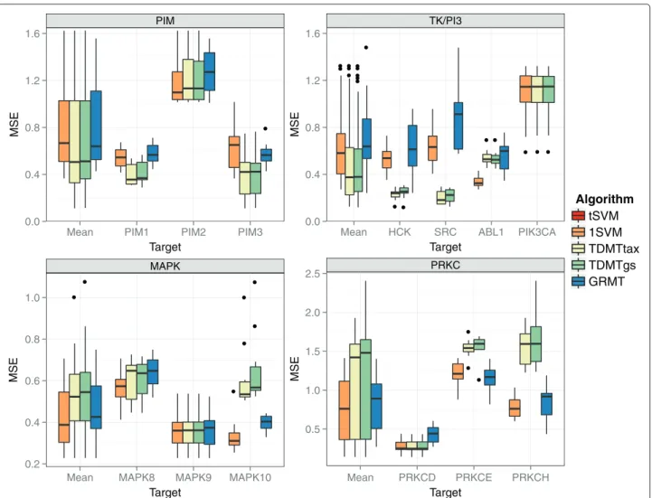
The results on the kinase subsets are presented in Figure 8. Additional results, such as the performance with respect to the scaffold or when using an ECFP encod-ing with depth 2 (ECFP_4), can be found in Additional file 3. For all subsets, but the MAPK subset, the multi-task approaches achieved a significantly better mean perfor-mance than the baseline methods 1SVM and tSVM. For the MAPK and PIM set, GRMT performed best, whereas TDMTtax achieved the lowest MSE for the TK/PI3 and PRKC set. Compared to the tSVM baseline, the best multi-task approach decreased the MSE by 26% for the MAPK subset up to 43% for the TK/PI3 subset. Zoom-ing in on the targets of the subsets, the performance gain of the best multi-task approach compared to the tSVM ranged from 16% for MAPK9 up to 56% for SRC. At least one multi-task algorithm obtained a significantly better performance than thetSVM for all targets except PIK3CA.

PIK3CA is part of the TK/PI3 kinase subset. The com-position of this set is different compared to the other 3 subsets. While the other subsets comprise targets of the same subfamily, the TK/PI3 set contains kinases of 2 different TK subfamilies and the atypical, taxonomically distant kinase PIK3CA. However, PIK3CA is structurally similar to the eukaryontic protein kinases [24,44]. The taxonomical relationships between PIK3CA and the other 3 targets were reflected in relatively low Spearman cor-relations between the target values (0.35-0.45). TDMTgs could not significantly improve the performance com-pared to the tSVM for this target because of the low task similarity. GRMT and TDMTtax performed equally to the tSVM because the similarity to PIK3CA was set to zero by the taxonomy. Supplying GRMT and TDMT-tax with the Spearman correlations resulted in a small but non-significant performance gain for both algorithms.

3 2

ABL1

SRC HCK

1

PIK3CA 2

1

MAPK9

MAPK10 MAPK8

PIM

TK/PI3 MAPK PRKC

Figure 7Taxonomies of kinase subsets.Taxonomies of the kinase subsets that were supplied to the multi-task algorithms. Each taxonomy is a subtree of the humane kinome tree.

values, the exact value ofBjust needs to be large enough for the TK taxonomy nodes to allow for knowledge trans-fer between the tasks. In the given human kinome tree, even taxonomically long branches induced a similarity parameterB>0.5.

On the PIM subset the multi-task approaches achieved a significantly lower MSE compared to thetSVM for all targets. The MSE of the 1SVM is considerably higher on PIM2 than on PIM1 and PIM3. The taxonomy based task similarities indicate that PIM2 is more distantly

PIM

0.0 0.5 1.0

Mean PIM1 PIM2 PIM3

Target

MSE

MAPK

0.0 0.3 0.6 0.9

Mean MAPK8 MAPK9 MAPK10

Target

MSE

TK/PI3

0.0 0.5 1.0

Mean HCK SRC ABL1 PIK3CA

Target

MSE

PRKC

0.0 0.3 0.6 0.9

Mean PRKCD PRKCE PRKCH

Target

MSE

Algorithm tSVM 1SVM TDMTtax TDMTgs GRMT

related to PIM1 and PIM3 than they are related to each other. Additionally, inhibitors often exhibit a higher affin-ity against both PIM1 and PIM3 than against PIM2 [54], which is reflected by the pIC50 values of the subsets. We conjecture that the 1SVM mainly learned the structure-activity relationships based on the training data of PIM1 and PIM3, which lead to a worse performance on PIM2 because the mean pIC50 values differ by about 0.8. In con-trast to the 1SVM, the multi-task approaches could exploit the taxonomy of the PIM kinases and adapt to differences in the target values, which improved the MSE. Gener-ally, the 1SVM should achieve a high MSE when there are considerable differences in the mean pIC50 of the targets. For the MAPK subset, the multi-task learners achieved the smallest performance gain. The 1SVM performed considerably worse than thetSVM for MAPK8, which is similar to the behavior on the PIM subset. However, lit-erature [55], the high taxonomy based task similarities (0.87-0.95), and the pIC50 values of the targets indicate a reasonably high similarity between the tasks. An expla-nation might be the considerably larger variance of the pIC50 values for MAPK8. The 1SVM mainly adapted to the applicability domain of MAPK9 and MAPK10, which does not include the larger pIC50 range of MAPK8. Inter-estingly, GRMT and TDMTgs performed significantly better than thetSVM on all targets of the subset, whereas TDMTtax performed similar to the tSVM except for MAPK9. This behavior indicates that the supplied taxon-omy is suboptimal. We evaluated an alternative taxontaxon-omy, which we generated with UPGMA from the Spearman correlations between the pIC50 values. The alternative taxonomy did have slightly lower task similarities and the positions of MAPK9 and MAPK8 were swapped (see Figure 9). Supplied with this taxonomy TDMTtax also

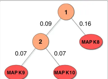
2

1

MAP K8

0.07

0.07

0.09

0.16

MAP K10 MAP K9

Figure 9Alternative taxonomy for the MAPK subset.The alternative taxonomy was generated with UPGMA from the Spearman correlations between the pIC50 values of the MAPK subset targets.

performed significantly better on MAPK8 and MAPK10 (see Additional file 3). The performance of TDMTgs also slightly increased with this alternative taxonomy on all targets but MAPK9. These results show that the topology of the taxonomy matters for top-down approaches.

On the PRKC subset, the multi-task algorithms achieved a significantly better performance than the tSVM on all subsets. For PRKCD, the 1SVM achieved a lower median MSE than the multi-task approaches. How-ever, this difference was non-significant. Like on the PIM subset, the mean pIC50 of PRKCE is about 0.6 lower than the mean pIC50 of the other targets, which resulted in a high MSE for the 1SVM on PRKCE. TDMTgs performed considerably worse than TDMTtax for all targets. The pIC50 values of PRKCE and PRKCH are dissimilar com-pared to the similarity to PRKCD. The grid search chose B ≤ 0.1 for the parent taxonomy node of PRKCE and PRKCH for 4 out of 10 repetitions. Given these parame-ter settings, PRKCE and PRKCH could not profit from the pIC50 value similarity to PRKCD. Furthermore, the grid search yieldedB≤ 0.25 for 5 out of 10 runs for PRKCD, which resulted in a small profit for PRKCD. Optimizing bothCandBresulted in overfitted parameter values for TDMTgs that do not generalize well. TDMTtax is less prone to overfitting because it only searches forCin a grid search.

Overall the results show that the multi-task algorithms are promising methods for inferring multi-target QSAR models. However, each of the algorithms has its draw-backs. While GRMT and particularly TDMTtax rely on sensible taxonomies, TDMTgs is prone to overfitting parameter values for small data sets.

mainly the same laboratory, whereas the data of the PRKC subsets stems from several different studies conducted by different laboratories.

To evaluate the predictive power of multi-task learning with respect to novel targets, we performed a leave-one-sequence-out validation, which puts aside the data of a certain target for external testing while using the data of the remaining targets for training. To keep comparability to the previous setup, we used the same 25 test com-pounds of a target as in the previous experiments. Further-more, the training sets had the same size as in the previous setup. To account for putting aside one target, the remain-ing targets received more trainremain-ing instances. Like before, we generated 10 different splits, which resulted in 10 different performance values per left out target.

The multi-task methods had to be adapted for the pre-diction of novel targets. For the TDMT approaches, the parent model of the left out target leaf was used for the prediction because a leaf model cannot be inferred without training instances. In the GRMT formulation, we adapted the graph LaplacianL, such that the GRMT does not regularize the model complexity (wt2) of a targett without training instances, but only forces the similarity to other models (Astws−wt2).

The results of the leave-one-sequence-out experiments are depicted in Figure 10. The results show that the 1SVM exhibits a similar behavior compared to GRMT, which is different to the behavior of both top-down approaches. On 3 targets GRMT and the 1SVM perform considerably better, whereas the top-down approaches achieved a bet-ter MSE for 4 targets. Furthermore, there is always one target per subset on which the TDMT methods perform equal to the 1SVM (PIM2, PIK3CA, MAPK9, PRKCD) because the parent node of the corresponding leaf is the root, and training the root is equal to training the 1SVM. Generally, the results indicate that it is often better to train the 1SVM instead of the GRMT approach. An explana-tion for this behavior is, that based on the small number of targets in a kinase subset, it is better to exploit as much knowledge from the other targets as possible. For data sets with more targets and a deeper taxonomy, there might be a difference between the 1SVM and GRMT. Comparing the results to the previous evaluation setup indicates that the knowledge transfer to novel targets does only work considerably well for highly similar targets (e.g. HCK, SRC). Zooming in on the details shows that one of the main problems for the prediction of novel targets is a shift in the bias. On PIM1 and PIM3, the leave-one-sequence-out results of the TDMT algorithms are similar to the results of the previous evaluation (see Figure 8), whereas the approaches performed considerably worse for PIM2. Differences in the bias might also be the explana-tion for the difference between the top-down approaches and GRMT/1SVM because the TDMT methods calculate

a new pIC50 bias for each node, whereas GRMT/1SVM calculate an average bias over all training instances.

Kinome

In the final experiment, we evaluated the five algorithms on the whole kinome data using the human kinome tree as taxonomy. We assessed the performance with a 3-fold nested cross-validation that we repeated 3 times. Hence, we obtained 9 performance evaluations per algorithm and target. The data set preparation of the kinome data required at least 15 compounds for each target. Conse-quently, a 3-fold outer cross-validation ensures a test set size of≥5. For the model selection, we employed a 2-fold inner cross-validation, again to ensure a test set size of at least 5.

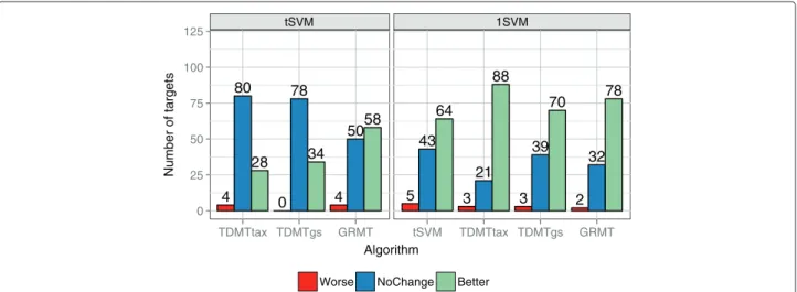
Figure 11 summarizes the results of the multi-task approaches compared to the baseline methods. Detailed results for all 112 kinase targets are depicted in Additional file 4. As to be expected, the 1SVM baseline had the worst performance on most of the data sets because the proteins of the kinome are substantially different. It obtained a con-siderably higher MSE on the majority of the targets. The 1SVM obtained a non-significantly different performance to thetSVM on 43 targets and to the multi-task algorithms on 21 targets for TDMTtax up to 39 targets for TDMTgs. On ERBB4 all other algorithms performed worse than the 1SVM. ERBB4 is a small set (39) whose compounds highly overlap with compounds of the large sets EGFR (1104) and ERBB2 (962). The overlapping molecules exhibit a high correlation between the pIC50 values (≈ 0.8). We think that the combination of the overlap, the high target value similarity, and possibly a restriction to a small part of the chemical space enabled the 1SVM to learn the task better than the other approaches.

Looking at the differences to the tSVM, GRMT per-formed best. It obtained a significantly lower MSE for the majority of the data sets, followed by TDMTgs, which achieved a lower MSE for a third of the targets. TDMT-tax exhibited the worst performance of the multi-task algorithms and performed significantly better for only 28 targets. However, zooming in on the SRC subfamily TDMTtax achieved the best results on HCK, LYN, and YES1 and decreased the MSE by 48−75% compared to thetSVM. A similar behavior on the SRC subfamily was observed on the TK/PI3 kinase subset. The SRC subfam-ily tree of the human kinome taxonomy approximates the task similarities well.

Algorithm tSVM 1SVM TDMTtax TDMTgs GRMT PIM

0.0 0.4 0.8 1.2 1.6

Mean PIM1 PIM2 PIM3

Target

MSE

TK/PI3

0.0 0.4 0.8 1.2 1.6

Mean HCK SRC ABL1 PIK3CA

Target

MSE

MAPK

0.2 0.4 0.6 0.8 1.0

Mean MAPK8 MAPK9 MAPK10

Target

MSE

PRKC

0.5 1.0 1.5 2.0 2.5

Mean PRKCD PRKCE PRKCH

Target

MSE

Figure 10Leave-one-sequence-out performance on kinase subsets.Mean squared error (MSE) for leave-one-sequence-out validation. Each boxplot depicts the performance of a leave-one-sequence-out validation performed on 10 random splits. The target “Mean” includes the data of all targets. For PIK3CA, the GRMT performance was not evaluated because the task similarity to the other targets was zero.

(0.32). Similar to the 1SVM, GRMT centers the pIC50 val-ues using the average over all tasks. It has to encode the bias between the average pIC50 values of the tasks using the features contained in the training compounds of the tasks. However, it might not be possible to encode the bias well, which results in a higher MSE. Thus, for taxo-nomically similar tasks with substantially different median pIC50 values GRMT potentially encounters difficulties. In contrast, the TDMT algorithms center the pIC50 val-ues for each taxonomy node separately, which allows to easily adapt to changing average pIC50 values. However, this behavior results in less comparable weights between the nodes because the bias of the pIC50 values is not encoded by features of the compounds of the tasks. The problem of differing average pIC50 values between tasks can be circumvented for GRMT by adding a regularized bias term as shown in Equation 7. Another possibility is to skip the feature selection, which removes features that

occur in more than 90% of the compounds. The weight of these features can act as implicit bias terms. Evaluating the performance of GRMT without feature selection resulted in a comparable performance to the tSVM on MAPK3 (see Additional file 4). Still, one should be cautious when using multi-task regression given tasks with considerably differing average target values.

0 25 50 75 100 125

Number of targets

tSVM 1SVM

4 80

28

0 78

34

4 5058

5 43

64

3 21

88

3 39

70

2 32

78

TDMTtax TDMTgs GRMT tSVM TDMTtax TDMTgs GRMT Algorithm

Worse NoChange Better

Figure 11Comparison of algorithms to baseline methods on kinome data.Summary of the differences between each algorithm and baseline methods on the 112 kinase targets. The left graph shows the summary compared to thetSVM baseline, the right graph compared to the 1SVM baseline. “Worse” denotes a significantly higher MSE compared to a baseline method, “NoChange” non-significant changes, and “Better” a significantly lower MSE.

existing target descriptors used in proteochemometric modeling.

As shown on the simulated data, the benefit of multi-task learning depends on the model complexity, the num-ber of training instances of a task, and the availability of a similar target. Given at least one target with suffi-cient similarity (≥ 0.8), GRMT decreased the MSE by 20% for targets with less than 100 compounds, whereas the decrease was only 6% on average for targets with at least 100 compounds. Hence, out-of-domain knowledge from other targets is mainly beneficial when not enough in-domain knowledge is available. In order to check the possible benefit of multi-task learning, we can compute a learning curve (e.g. number of compounds vs. MSE) as suggested in [22]. If the curve reaches saturation, multi-task learning is likely not beneficial. Furthermore, the benefit increases for targets with a small amount of in-domain knowledge that are similar to a target with a lot of compounds, like for YES1 in the SRC subfamily. The YES1 set comprises 37 compounds, whereas the taxonomically highly related target SRC contains 1610 compounds.

Finally, it should be mentioned that the multi-task algorithms are not designed for simultaneously inferring QSAR models on tasks as diverging as the whole kinome, but rather one should focus on a subset of desired targets.

Conclusions

In this study, we presented two multi-task SVR algo-rithms and their application on multi-target QSAR mod-els to support the optimization of a lead candidate in multi-target drug design. The first method, top-down domain adaption multi-task (TDMT) SVR, successively trains more specific models along a supplied taxonomy.

For TDMT the branch lengths of the taxonomy can be supplied by the user or approximated by a grid search during training. The second method, graph-regularized multi-task (GRMT) SVR, assumes the tasks to be pairwise related with a given similarity and trains all task models in one step. The training time of both algorithms is linear in the number of training instances and tasks.

We evaluated the two TDMT SVR variants and the GRMT SVR on simulated data and on a data set of human kinases assembled from the database ChEMBL. Furthermore, we examined the behavior of the employed methods on selected subsets of the kinome data set. The results show that multi-target learning results in a con-siderable performance gain compared to training separate SVR models if knowledge can be transferred between sim-ilar targets. However, the performance increases only as long as not enough in-domain knowledge is available to a task for solving the underlying problem. Generally, QSAR problems are complex and high dimensional such that a considerable performance gain is apparent as long as there is sufficient similarity between the tasks, which, in partic-ular, is the case for the kinase subfamilies. Yet, if the tasks are too similar it can be worthwhile to regard the models as identical and train a simple SVM with all data, as done by the 1SVM.