Lecture 6
Random variable
Plan of the lecture:
1. Discrete random variable
1.1Definitions of random variable and discrete random variable
1.2Probability mass function
2. Continuous random variables and PDFs
3. Cumulative distribution functions
1 Discrete Random variable
1.1 Definitions of random variable and discrete random variable
In many probabilistic models, the outcomes are of a numerical nature, e.g., if they
correspond to instrument readings or stock prices. In other experiments, the outcomes are not
numerical, but they may be associated with some numerical values of interest. For example, if
the experiment is the selection of students from a given population, we may wish to consider
their grade point average. When dealing with such numerical values, it is often useful to assign
probabilities to them. This is done through the notion of a random variable.
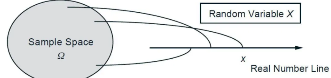
Given an experiment and the corresponding set of possible outcomes (the sample space),
a random variable associates a particular number with each outcome; see Fig. 1. We refer to this
number as the numerical value or the experimental value of the random variable.
Mathematically, a random variable is a real-valued function of the experimental outcome.
Figure 1: Visualization of a random variable. It is a function that assigns a numerical value to
each possible outcome of the experiment.
Here are some examples of random variables:
(a) In an experiment involving a sequence of 5 tosses of a coin, the number of heads in
the sequence is a random variable. However, the 5-long sequence of heads and tails is not
considered a random variable because it does not have an explicit numerical value.
(b) In an experiment involving two rolls of a die, the following are examples of random
variables:
(1) The sum of the two rolls.
(2) The number of sixes in the two rolls.
(c) In an experiment involving the transmission of a message, the time needed to transmit
the message, the number of symbols received in error, and the delay with which the message is
received are all random variables.
There are several basic concepts associated with random variables, which are
summarized below.
Main Concepts Related to Random Variables
Starting with a probabilistic model of an experiment:
A random variable is a real-valued function of the outcome of the experiment.
A function of a random variable defines another random variable.
We can associate with each random variable certain “averages” of interest, such the
mean and the variance.
A random variable can be conditioned on an event or on another random variable.
There is a notion of independence of a random variable from an event or from another
random variable.
A random variable is called discrete if its range (the set of values that it can take) is
finite or at most countably infinite. For example, the random variables mentioned in (a) and (b)
above can take at most a finite number of numerical values, and are therefore discrete.
A random variable that can take an uncountably infinite number of values is not discrete.
Concepts Related to Discrete Random Variables
Starting with a probabilistic model of an experiment:
A discrete random variable is a real-valued function of the outcome of the experiment
that can take a finite or countably infinite number of values.
A (discrete) random variable has an associated probability mass function (PMF), which gives the probability of each numerical value that the random variable can take.
A function of a random variable defines another random variable, whose PMF can be
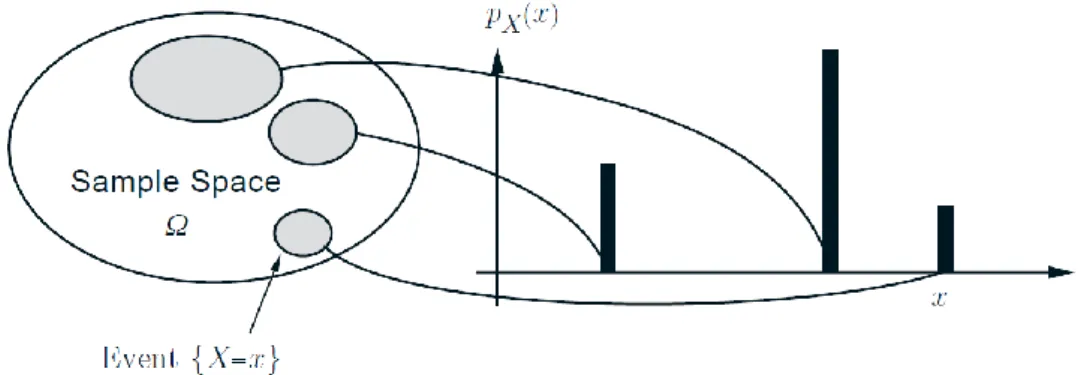
Figure 2: Example of discrete RV
1.2 Probability mass function
The most important way to characterize a random variable is through the probabilities of
the values that it can take. For a discrete random variable 𝑋, these are captured by the
probability mass function (PMF for short) of 𝑋, denoted 𝑝𝑋. In particular, if 𝑥 is any possible
value of 𝑋, the probability mass of 𝑥, denoted 𝑝𝑋(𝑥), is the probability of the event {𝑋 = 𝑥}
consisting of all outcomes that give rise to a value of 𝑋 equal to 𝑥:
𝑝𝑋 𝑥 = 𝑃 𝑋 = 𝑥 .
For example, let the experiment consist of two independent tosses of a fair coin, and let 𝑋
be the number of heads obtained. Then the PMF of 𝑋 is
𝑝𝑋 𝑥 = 1 41 2 𝑖𝑓 𝑥 = 0 𝑜𝑟 𝑥 = 2, 𝑖𝑓 𝑥 = 1,
0 𝑜𝑡ℎ𝑒𝑟𝑤𝑖𝑠𝑒.
In what follows, we will often omit the braces from the event/set notation, when no
ambiguity can arise. In particular, we will usually write 𝑃(𝑋 = 𝑥) in place of the more correct
0 5 10 15 20 25 30
01.02.10 06.02.10 11.02.10 16.02.10 21.02.10 26.02.10 03.03.10 08.03.10 13.03.10 18.03.10
notation 𝑃( 𝑋 = 𝑥 ).We will also adhere to the following convention throughout: we will use
upper case characters to denote random variables, and lower case characters to denote real
numbers such as the numerical values of a random variable.
Note that
𝑝𝑥 𝑋 𝑥 = 1,
where in the summation above, 𝑥 ranges over all the possible numerical values of 𝑋. This
follows from the additivity and normalization axioms, because the events {𝑋 = 𝑥} are disjoint
and form a partition of the sample space, as 𝑥 ranges over all possible values of 𝑋. By a similar
argument, for any set 𝑆 of real numbers, we also have
𝑃 𝑋 ∈ 𝑆 = 𝑥∈𝑆𝑝𝑋 𝑥 .
For example, if 𝑋 is the number of heads obtained in two independent tosses of a fair
coin, as above, the probability of at least one head is
𝑃 𝑋 > 0 = 𝑥>0𝑝𝑋 𝑥 = 12+14 =34.
Calculating the PMF of 𝑋 is conceptually straightforward, and is illustrated in Fig. 3.
Figure 3: Illustration of the method to calculate the PMF of a random variable 𝑋. For each
possible value 𝑥, we collect all the outcomes that give rise to 𝑋 = 𝑥 and add their probabilities to
obtain 𝑝𝑋 𝑥 .
Calculation of the PMF of a Random Variable 𝑋
1. Collect all the possible outcomes that give rise to the event {𝑋 = 𝑥}.
2. Add their probabilities to obtain 𝑝𝑋(𝑥).
2 Continuous random variables and PDFs
A random variable 𝑋 is called continuous if its probability law can be described in terms
of a nonnegative function 𝑓𝑋, called the probability density function of 𝑋, or PDF for short,
which satisfies
𝑃(𝑋 ∈ 𝐵) = 𝑓𝐵 𝑋(𝑥)𝑑𝑥,
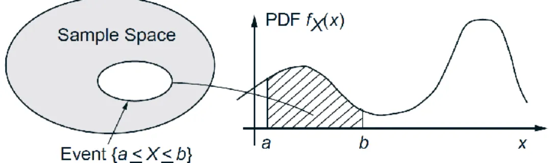
for every subset 𝐵 of the real line.In particular, the probability that the value of 𝑋 falls within an
interval is
𝑃(𝑎 ≤ 𝑋 ≤ 𝑏) = 𝑓𝑎𝑏 𝑋(𝑥)𝑑𝑥,
and can be interpreted as the area under the graph of the PDF (see Fig. 4). For any single value a,
we have 𝑃(𝑋 = 𝑎) = 𝑓𝑎𝑎 𝑋(𝑥)𝑑𝑥 = 0. For this reason, including or excluding the endpoints of
an interval has no effect on its probability:
𝑃(𝑎 ≤ 𝑋 ≤ 𝑏) = 𝑃(𝑎 < 𝑋 < 𝑏) = 𝑃(𝑎 ≤ 𝑋 < 𝑏) = 𝑃(𝑎 < 𝑋 ≤ 𝑏).
Figure 4: Illustration of a PDF. The probability that 𝑋 takes value in an interval [𝑎, 𝑏] is
𝑓𝑎𝑏 𝑋(𝑥)𝑑𝑥, which is the shaded area in the figure.
Note that to qualify as a PDF, a function 𝑓𝑋 must be nonnegative, i.e., 𝑓𝑋(𝑥) ≥ 0 for
𝑓−∞∞ 𝑋(𝑥)𝑑𝑥= 𝑃(−∞ < 𝑋 < ∞) = 1.
Graphically, this means that the entire area under the graph of the PDF must be equal to
1.
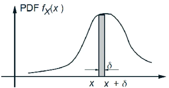
To interpret the PDF, note that for an interval [𝑥, 𝑥 + 𝛿] with very small length 𝛿, we
have
𝑃 [𝑥, 𝑥 + 𝛿] = 𝑥𝑥+𝛿𝑓𝑋(𝑡) 𝑑𝑡≈ 𝑓𝑋(𝑥) ∙ 𝛿,
so we can view 𝑓𝑋(𝑥) as the “probability mass per unit length” near x (cf. Fig. 5). It is
important to realize that even though a PDF is used to calculate event probabilities, 𝑓𝑋(𝑥) is not
the probability of any particular event. In particular, it is not restricted to be less than or equal to
one.
Figure 5: Interpretation of the PDF 𝑓𝑋(𝑥) as “probability mass per unit length” around 𝑥. If δ is
very small, the probability that 𝑋 takes value in the interval [𝑥, 𝑥 + 𝛿] is the shaded area in the
figure, which is approximately equal to 𝑓𝑋(𝑥) ∙ 𝛿.
Summary of PDF Properties
Let 𝑋 be a continuous random variable with PDF 𝑓𝑋:
𝑓𝑋(𝑥) ≥ 0 for all 𝑥.
𝑓−∞∞ 𝑋(𝑥)𝑑𝑥 = 1.
If 𝛿 is very small, then 𝑃 [𝑥, 𝑥 + 𝛿] ≈ 𝑓𝑋(𝑥) ∙ 𝛿. For any subset 𝐵 of the real line,
3 Cumulative distribution functions
We have been dealing with discrete and continuous random variables in a somewhat
different manner, using PMFs and PDFs, respectively. It would be desirable to describe all kinds
of random variables with a single mathematical concept. This is accomplished by the
cumulative distribution function, or CDF for short. The CDF of a random variable 𝑿 is
denoted by 𝑭𝑿 and provides the probability 𝑷(𝑿 ≤ 𝒙). In particular, for every 𝑥 we have
𝐹𝑋 𝑥 = 𝑃 𝑋 ≤ 𝑥 =
𝑝𝑋 𝑘
𝑥≤𝑘
𝑋: 𝑑𝑖𝑠𝑐𝑟𝑒𝑡𝑒,
𝑓𝑋 𝑡 𝑑𝑡
𝑥
−∞
𝑋: 𝑐𝑜𝑛𝑡𝑖𝑛𝑢𝑜𝑢𝑠.
Loosely speaking, the CDF 𝐹𝑋 𝑥 “accumulates” probability “up to” the value 𝑥.
Any random variable associated with a given probability model has a CDF, regardless of
whether it is discrete, continuous, or other. This is because {𝑋 ≤ 𝑥} is always an event and
therefore has a well-defined probability. Figures 6 and 7 illustrate the CDFs of various discrete
and continuous random variables. From these figures, as well as from the definition, some
general properties of the CDF can be observed.
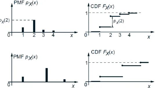
Figure 6: CDFs of some discrete random variables. The CDF is related to the PMF through the
formula 𝐹𝑋 𝑥 = 𝑃 𝑋 ≤ 𝑥 = 𝑥≤𝑘𝑝𝑋 𝑘 , and has a staircase form, with jumps occurring at the
values of positive probability mass. Note that at the points where a jump occurs, the value of 𝐹𝑋
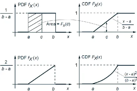
Figure 7: CDFs of some continuous random variables. The CDF is related to the PDF through
the formula 𝐹𝑋 𝑥 = 𝑃 𝑋 ≤ 𝑥 = 𝑓−∞𝑥 𝑋 𝑡 𝑑𝑡. Thus, the PDF 𝑓𝑋 can be obtained from the CDF
by differentiation: 𝑓𝑋 𝑥 =𝑑𝐹𝑑𝑥𝑋 𝑥 . For a continuous random variable, the CDF has no jumps, i.e.,
it is continuous.
Properties of a CDF
The CDF 𝐹𝑋 of a random variable 𝑋 is defined by 𝐹𝑋 𝑥 = 𝑃 𝑋 ≤ 𝑥 , for all 𝑥, and has
the following properties.
𝐹𝑋 is monotonically nondecreasing:
if x ≤ y, then 𝐹𝑋(𝑥) ≤ 𝐹𝑋(𝑦).
𝐹𝑋 𝑥 tends to 0 as 𝑥 → −∞, and to 1 as 𝑥 → ∞.
If 𝑋 is discrete, then 𝐹𝑋 has a piecewise constant and staircase-like form.
If 𝑋 is continuous, then 𝐹𝑋 has a continuously varying form.
If 𝑋 is discrete and takes integer values, the PMF and the CDF can be obtained from
each other by summing or differencing:
𝐹𝑋 𝑘 = 𝑘𝑖=−∞𝑝𝑋 𝑖 ,
𝑝𝑋 𝑘 = 𝑃 𝑋 ≤ 𝑘 − 𝑃 𝑋 ≤ 𝑘 − 1 = 𝐹𝑋 𝑘 − 𝐹𝑋 𝑘 − 1 ,
for all integers 𝑘.
If 𝑋 is continuous, the PDF and the CDF can be obtained from each other by
integration or differentiation:
𝐹𝑋 𝑥 = 𝑓−∞𝑥 𝑋 𝑡 𝑑𝑡,
𝑓𝑋 𝑥 =𝑑𝐹𝑋
𝑑𝑥 𝑥 .