Dielectric Decrement for Aqueous NaCl Solutions: E
ff
ect of Ionic
Charge Scaling in Nonpolarizable Water Force Fields
Sayan Seal,
†Katharina Doblho
ff
-Dier,
†and Jo
̈
rg Meyer
*
Gorlaeus Laboratories, Leiden Institute of Chemistry, Leiden University, PO Box 9502, 2300 RA Leiden, The Netherlands
*
S Supporting InformationABSTRACT: We investigate the dielectric constant and the dielectric decrement of aqueous NaCl solutions by means of molecular dynamic simulations. We thereby compare the performance of four different force
fields and focus on disentangling the origin of the dielectric decrement and the influence of scaled ionic charges, as often used in nonpolarizable force
fields to account for the missing dynamic polarizability in the shielding of electrostatic ion interactions. Three of the force fields showed excessive contact ion pair formation, which correlates with a reduced dielectric
decrement. In spite of the fact that the scaling of charges only weakly influenced the average polarization of water molecules around an ion, the rescaling of ionic charges did influence the dielectric decrement, and a close-to-linear relation of the slope of the dielectric constant as a function of concentration with the ionic charge was found.
1. INTRODUCTION
Electrolytic solutions and the solid−electrolyte interface are of importance in biological systems as well as for various chemical applications, such as batteries, and in the electrochemical industry. The computational modeling of electrolytes and solid−electrolyte interfaces is, however, challenging due to the large amount of atoms and molecules that need to be simulated. Implicit solvation models augmented by (modified) Poisson−Boltzmann models to account for nonzero ionic strength provide a computationally cheap workaround.1,2 These continuum models alleviate the need for thermody-namic sampling of the electrolyte degrees of freedom. On the downside, these models commonly require a parametrization, and the fitted parameters are often not transferable (e.g., between neutral solutes and charged solutes3 or between molecules and surfaces4,5). Even when using available experimental data as “parameters” (e.g., the concentration-and temperature-dependent dielectric constant of the electro-lyte), implicit solvation models systematically fail at high ion concentrations when the atomistic nature of the solvent becomes important.6 Force-field-based molecular dynamics calculations on the other hand provide a comparatively cheap option to access the solvent degrees of freedom explicitly. It is, however, nontrivial to devise forcefields that correctly describe important properties such as the solubility, density-over-temperature curves at different ionic concentrations, and activity coefficients.7−9
Most available and commonly used electrolyte force fields combine nonpolarizable water models with Lennard-Jones and Coulomb interactions for the ion−ion and water−ion interactions. In recent years, it has, however, been realized that this approach generally leads to an incorrect prediction of diffusivity constantsa fact that Kann and Skinner10 have remedied by rescaling the ionic charges. This rescaling of
charges was originally proposed by Leontyev and Stuche-brukhov.11 It is based on the idea of phenomenologically including the effect of an electronic dielectric continuum contribution to the polarizability in classical molecular dynamics.12 Leontyev and Stuchebrukhov have coined this the molecular dynamics electronic continuum (MDEC) model,11,12which has also been referred to as the electronic continuum correction (EEC) method.13 It has been widely used with good results,9,14 for example, for the structure of concentrated ionic solutions,13 electronic conductivity,15 as well as solvation and ion pairing.16The rescaled charges should account for the missing static polarizability of the water in the forcefield but could cause other undesired effects: for example, when ions sample regions in space that have a polarizability different from that of water or when ion association becomes important at high concentrations.10 Addressing the latter concern, Benavides et al.17showed that while the scaling of ion charges has a considerable effect on the free energy of the solid, the melting temperature can still be captured correctly by scaled ion force fields. In the present paper, we want to investigate the influence of the ion scaling approach on the dielectric decrement, that is, the reduction of the dielectric constant of water with increasing ion concentration.
The fact that solvated ions can influence the dielectric constant of the solvent was already recognized in the early 20th century18and was rigorously studied experimentally by Hasted et al.19 for a large number of salts and wide concentration ranges. For NaCl, they found a linear dielectric decrement at low concentrations that levels offat concentrations above 2 M. A tentative explanation of this effect, which is actually still in
Received: August 19, 2019
Revised: October 22, 2019
Published: October 24, 2019
Article pubs.acs.org/JPCB
Cite This:J. Phys. Chem. B2019, 123, 9912−9921
Derivative Works (CC-BY-NC-ND) Attribution License, which permits copying and redistribution of the article, and creation of adaptations, all for non-commercial purposes.
Downloaded via LEIDEN UNIV on November 25, 2019 at 12:32:33 (UTC).
line with today’s commonly accepted explanation, was already put forward by Blüh18in 1924. The basic idea is that, in the vicinity of an ion, the water dipoles will rather align along the
field created by the ion than react to an external field. As a result of this, the water molecules in the so-formed solvation shell will not contribute to the dielectric response18,20 or contribute to a lesser extent21than“free”water molecules, thus lowering the dielectric constant. This effect can be expected to be linear with concentration as long as the concentrations are low. At higher concentrations, volume exclusion effects,22,23as well as effects of overlapping hydration shells,24 ion−ion correlations (dressed ions),25,26 ion−ion correlations beyond the mean field,23,27 ion pair formation,28 and ion polar-izabilities29may become important. Alternatively (or additally), the dielectric decrement may also be caused by an ion-induced breakdown of dipole−dipole correlation, as put forward by Rinne et al.30Such a breakdown in dipole−dipole correlation would reduce the Kirkwood g factor31 and thus reduce the dielectric constant.
Although most force fields suffer from an incorrect representation of the dielectric constant at zero ionic strength, the effect of the dielectric decrement can be captured astonishingly well on the force field level (see, e.g., refs 30,
32−37). Remarkable accuracy, even at high concentrations, can be obtained with forcefields optimized toward the correct representation of the dielectric constant.38
In spite of a plethora of force-field-based studies on the dielectric decrement, there are only a few comparative studies, and several questions remain.
1. How far is the observed dielectric decrement influenced by the forcefield used?
2. Will the decrement diminish if the ionic charges are rescaled?
3. Are our observations more in line with an effect of dielectric saturation close to the ions, or may the decrement indeed be influenced more strongly by the breakdown of water correlation as suggested by Rinne et al.?30
To answer these questions, we simulate the dielectric constant at different concentrations of NaCl between 0 and 5 M using 4 different forcefields, two of them with ionic charges equal to qion=±1.0eand two with scaled ionic charges ofqion=±0.85e. The paper is organized as follows. InSection 2, we describe the computational methods, including the different FF parameters, the details regarding the computational setup, the procedure to calculate the dielectric constant, and the analysis of the MD data. Then, we present our results for the dielectric constant at different temperatures and ionic concentrations, discuss ion-pairing effects, and analyze the influence of rescaled ionic charges in Section 3, which is followed by the conclusions inSection 4.
2. METHODS
2.1. Force Fields.All forcefields that are used in this work describe interactions among and between (rigid) water molecules and the sodium and chloride ions based on Coulomb
π
= ϵ
V
q q
r 1 4 ij
i j
ij Coul
0 (1)
whereϵ0is the vacuum permittivity, and 12-6 is Lennard-Jones (LJ)
Ä
Ç ÅÅÅÅÅ ÅÅÅÅÅ ÅÅÅ i
k jjjjj j
y
{ zzzzz z
i
k jjjjj j
y
{ zzzzz z É
Ö ÑÑÑÑÑ ÑÑÑÑÑ ÑÑÑ
γ σ σ
= −
V
r r
4
ij ij
ij
ij
ij
ij LJ
12 6
(2)
(pair) potentials. Here, the indicesi andjrefer to H and O atoms as well as Na+ and Cl− ions, and rij is the distance between the pair (i,j). The atomic and ionic chargesqifor the Coulomb interaction and the well depth γij and distance parametersσijappearing in the LJ potential are tabulated in full detail in theSupporting Informationfor the four different force
fields employed in this study. Here, we only summarize the essential distinguishing features.
• CC (qion = ±1e): This force field is based on ion parameters determined by Smith and Dang byfitting to energies of small clusters.39Since we combine the ionic parameters with SPC/E40 as a water force field, as proposed by Chowdhuri and Chandra,33we refer to this force field as “CC”. Deviating from what has been proposed by these authors, we use geometric combina-tion rules for the LJ potential parameters in this work.
• MP (qion=±1e): We also include a forcefield that relies on the ion parameters from Mao and Pappu41 (MP). These parameters are based purely on crystal lattice properties and are hence independent of the water force
field. We combine it with TIP4P/200542in the present work.
• MP-S (qion=±0.85e): Kann and Skinner10proposed to rescale the ionic charges appearing in the MP forcefield to account for the lack of static polarizability in TIP4P/ 2005.42This scaled MP forcefield (termed MP-S in the following) is thus equivalent to MP, except for the fact that the ion charges are scaled by a factor 0.85.
• BPCEAV (qion = ±0.85e): This recent force field by Benavides et al.17 (our acronym results from the first letter of the authors’ last names) is also based on TIP4P/200542and employs ionic charges scaled by 0.85. BPCEAV differs from MP-S because it has been fitted more carefully to properties of the ionic solution. 2.2. Molecular Dynamics Simulations. All molecular dynamics (MD) simulations were performed using the LAMMPS code.43 Cubic boxes with box length L = 25.5 Å (i.e., with volume V= L3) were used. The number of water molecules was adjusted to match the experimental values for the density of NaCl solutions at different molarities at 300 K. We studied a large range of ionic concentrationsc ∈ 0.0, 0.1, 0.2, 0.5, 1.0, 1.5, 2.0, 2.5, 3.0, 4.0, and 5.0 M. At zero ionic strength (c= 0 M), the box contained NH2O = 556 water molecules corresponding to a densityρH2O= 0.99 g/cm3.
typical runtime of an entire simulation (both equilibration and thermodynamic sampling together) for any concentration was 13 hours, parallelizing 16 physical cores of two eight-core Xeon E5-2630 CPUs residing in the same compute node and using the standard spatial decomposition implemented in LAMMPS.43 2.3. Dielectric Constant. In a pure dipolar solvent, the dielectric constant can be obtained from the linear response theory50according to
ϵ = + ⟨ ⟩ − ⟨ ⟩ ϵ Vk T M M 1 3 2 2
B 0 (3)
wherekBis the Boltzmann constant,Tis the temperature, and M denotes the sum over all dipole moments pi in the simulation cell. Here and in the following, ⟨·⟩ denotes time averages.
In the presence of ions, the situation becomes more complicated. The only measurable quantity then becomes the frequency-dependent dielectric susceptibility, χ(ω), and dynamic cross-terms in the solution dielectric functionϵ(ω) as well as purely ionic terms would have to be taken into account in calculating the dielectric susceptibility.30,51Capturing these effects at the low-frequency limit is, however, computationally extremely challenging.30 The influence of kinetic cross-terms33,52 and ion contributions30,35 on the dielectric susceptibility can be expected to be small as long as ion paring, which can significantly enhance the low-frequency dielectric susceptibility, is negligible.35 As discussed in more detail in Section 3.4, the ion-pairing times observed for the forcefield discussed in this paper are such that an influence on the dielectric response cannot be ruled out for certain without calculating the dielectric response. However, rather than aiming at a full reproduction of the dielectric spectrum, in the present contribution, we are specifically interested in the effect of different forcefields on the dielectric decrement and, especially, to what extent the scaling of ionic charges influences dielectric decrement. We therefore do not aim at a full, computationally challenging, simulation of the dielectric susceptibility. Instead, we follow the commonly adopted approach36,38to limit our simulations to computing the static solution dielectric constantϵas defined ineq 3(i.e., neglecting dynamic cross-terms toϵand ion contributions toχ).
In computingeq 3, we take advantage of the fact that⟨M⟩= 0. (Note that this is only true if atoms constituting a single water molecule are taken from adjacent periodic cells using a minimum distance convention.) Test calculations showed that taking the statistical average of ⟨M⟩ into account does not significantly influence our result, proving that ⟨M⟩ is well converged to zero for the simulation times used.
Generally, the convergence of time-averaged quantities (like
ϵ as defined by eq 3) is judged based on plots of the cumulative average, which should stabilize if the sampling time is long enough. From such plots, it is, however, difficult to estimate error bars for the averaged quantity. To obtain statistical error bars for our estimates ofϵ, we therefore make use of a reblocking analysis.53 This allows us to estimate a value for the correlation-corrected standard deviationσ of the observable. To this end, we first compute estimators of the standard error for different block lengthsM= 1, 2, 4, 8, ... of the observablex=⟨x⟩
σ = ∑ ⟨ ⟩ − ⟨ ⟩ −
= x x
N ( ) ( 1) M i N M i M 1 2 , 2 M (4) where
∑
⟨ ⟩ = = − · · x M x 1 M ik i M
i M
k ,
( 1) (5)
andNMis the number of blocks of lengthMcontained in the time series xk with k ∈ [1, NM·M]. The value of σM will increase as long as serial correlation is still present and will stabilize at the correlation-corrected valueσ as soon asM is large enough. For very largeM, the estimate of σM becomes noisy. Making use of the python module pyblock,54 we automatically choose the ideal value ofMfor estimating σas suggested by Lee et al.55
To extract the excess polarization α, which defines the dielectric decrement at low concentrations, as well as the dielectric constant in the very high concentration (i.e., molten salt) limitϵms =ϵ(c→∞M), we fit our data forϵ(c) to an analytic model proposed by Gavish and Promislow.24
i k
jjjjj α y{zzzzz ϵ = ϵ − ϵ − ϵ ·
ϵ − ϵ
c L c
( ) w ( w ms) 3
w ms (6)
ϵw=ϵ(c= 0 M) is the dielectric constant of pure water (which we calculate separately and is thus not fit parameter). The functionL is given by
υ υ
υ
= −
L( ) coth( ) 1
(7)
For low concentrations,eq 6reduces to the linear equation as proposed by Hasted et al.19
α
ϵ( )c = ϵ −w c (8)
2.4. Ion Pairing.To quantify the pairing between Na+and Cl−ions, we calculate the coordination number
∫
π ρ= ′ ′ ′
+ − + + −
N ( )r 4 g ( )r r dr
r
Na Cl Na
0 Na Cl 2
(9)
where
∑ ∑
π ρ δ
= ⟨ | − | − ⟩ = = + − + + − g r
r r r r
( ) 1
4 i ( )
N
j N
i j
Na Cl 2
Na 1 1
Na Cl
(10)
is the radial distribution function (RDF) for the ion pair (Na+, Cl−),NNa+(NCl−) are the total numbers of Na+(Cl−) ions, and
ρ + =
+ N
V Na
Na
(ρ + =
− N
V Cl
Cl
particular ion pairi, jis in continuous close contact. If ioniis replaced by an ion i,̃ tijasc stops and a new tijasc̃ starts. Furthermore, ionsiand jcan pair multiple times during one simulation run, and ion j can be paired simultaneously with two counterionsiandi. While we believe this descriptor to bẽ relevant in the context of enhanced low-frequency dielectric response (seeSection 3.4), it should be kept in mind that the estimates for the mean ion association time will depend on the chosen cutoff distance and that the resulting pairing time distribution will be different from the average time during which an ionjis closely surrounded by at least one counterion i.
With this definition, we calculate the ion pair formation time distribution as
∑ ∑
∑
δ= −
= = =
+ −
+ −
+ −
p t
N N N t t
( ) 1 1 ( )
i N
j N
ij k N
ij k Na Cl
pair
Na Cl 1 1 1
, asc
ij
Na Cl
(11)
whereNijis the number of times that ioniforms an ion pair with ionj.
2.5. Water Dipole Alignment. The alignment of water molecules surrounding the Na+ and Cl−ions is characterized by
∑ ∑
δ=
| | ⟨= = · ̂ | ̂ | − ⟩
P r
N N r
p p r r
( ) 1 1 ( )
i N
j N
j ij ij
Xr
H O X H O 1 1
XO XO
2 2
X H2O
(12)
where X ∈ {Na+, Cl−}. This average dipole alignment P X r is
based on the projection of the individual water dipole
moments pj onto the radial unit vector ̂ = − | − |
rij
r r
r r
XO i j
i j
X O X O, which connects the ioniand the oxygen atom of the water molecule j. |pH2O|is the (static) magnitude of the dipole moment of a single water molecule, which differs for the different force
fields.
3. RESULTS AND DISCUSSION
3.1. Validation of Computational Setup.We start our discussion by validating the convergence ofϵwith respect to the simulated time interval of the MD simulations, which is shown inFigure 1 for the CC force field as a representative example. When usingeq 3to evaluate the dielectric constant,
relatively long simulations times are required to obtain satisfactory convergence.57 In our case, simulation times of 12 ns give satisfactory convergence. Other methods to compute ϵ may converge faster (see ref 58 for a recent comparison) but were deemed unnecessary here since 12 ns of simulation time for systems of the size considered here is nowadays easily accessible for force-field-based MD calcu-lations. In addition to the visual convergence check, we computed estimates for the standard deviations of the mean,σ, from a blocking analysis. We checked the reliability of these estimates by computing error bars to σ (error of the error). Independent of the force field, the corresponding relative errors do not considerably exceed 10%, thus providing confidence in our computational setup used to obtainσ.
Focusing on the minimum (c= 0 M, i.e., pure SPC/E water) and maximum (c= 5 M) concentrations, we have also checked the dependence of the calculated dielectric constants on system size by increasing the size of the cubic simulation boxes to box length L = 50.0 Å. The results shown inTable 1are identical within the statistical uncertainty. Consequently, the smaller box (L= 25.5 Å) is large enough to avoid errors forϵ that are caused byfinite size effects.
Our result for the dielectric constant of the CC forcefield at zero ionic strength (resulting in pure SPC/E water) ϵwCC =
ϵSPC/ E = 71.5 ± 1.9 is in good agreement with literature results.59The same holds true for MP, MP-S, and BPCEAV, all of which result in pure TIP4P/2005. For these cases, wefind
ϵwTIP4P= 59.3±1.3, in agreement with Abascal and Vega.42We emphasize here the known fact that SPC/E as well as TIP4P/ 2005 strongly underestimates ϵ, when compared with experimental results (ϵw = 78.3).56 This should be kept in mind during the following analysis of the dielectric decrement. 3.2. Temperature Dependence of Dielectric Con-stants. Before we turn to our results for the dielectric decrement obtained with the different forcefields, we briefly discuss whether its temperature dependence is relevant in the context of our MD simulations. Experimental data is available for temperatures ranging from 278 to 308 K and concen-trations between 0 and 5 M.60The factorT−1 in the second term ofeq 3leads to a“trivial”temperature dependence of our MD results for the dielectric constants. Thefluctuations of the total dipole momentMmay, however, also show a temperature dependence, which is in principle included in our MD simulations by the use of a thermostat. If this “nontrivial” temperature dependence ofϵis significant, then the dielectric decrement should be considered at different temperatures.
For a given data set of concentration-dependent dielectric constants, the aforementioned trivial temperature dependence can be eliminated by defining the temperature rescaled quantity
ϵ* = + [ϵ − ]
*
c T c T T
T ( ; ) 1 ( ; ) 1
(13) Figure 1.Dielectric constant (ϵ) as obtained with the CC forcefield
at 300 K for various ionic concentrationsc(colored lines). The result for pure water (ϵ(c= 0 M) =ϵw) is highlighted by the thick blue line, and the corresponding experimental value56(black horizontal line) is shown for comparison.
Table 1. Dielectric Constantϵas Obtained with the CC Force Field for Cubic Simulation Boxes with Different Box LengthsL for Different Concentrationsc. c= 0M
Corresponds to Pure SPC/E Water
for a given reference temperatureT*. We have plottedϵ*in
Figure 2forT*= 300 K as a function of concentration for 278,
300, and 308 K, again using the CC force field as a representative example. (The same trends are obtained for the other forcefields as well.) Considering the error bars in our calculations (see Section 3.1), we find the three solid lines corresponding to our MD data to overlap. Within the temperature range considered here, our MD simulations do not show any temperature dependence of the dipole
fluctuations, and the temperature dependence of the dielectric decrement is uniquely governed by the trivial temperature dependence included ineq 13. We have also appliedeq 13to the experimental data from Buchner et al.60that is available for
ϵ(c) at 278, 298, and 308 K and plotted the results inFigure 2
(dashed lines). A significant nontrivial temperature depend-ence is only observed experimentally forT< 300 K andc> 2 M, whereas the data forε*(c) almost overlaps at 298 and 308 K. This latter observation agrees with the predictions from the MD simulations at those temperatures.
Since the MD simulations did not show any nontrivial temperature dependence, we focus our analysis on the data obtained from MD simulations at 300 K.
3.3. Dielectric Decrement. As already indicated by the results presented before (Sections 3.1 and 3.2), our MD simulations predict a continuous decrease of the dielectric constant with increasing concentration. This is true not only for the CC forcefield discussed above but also for the other forcefields. A comparison of the resulting ϵ(c) is plotted in
Figure 3. For CC, MP, and MP-S, the dielectric decrement is
approximately linear only below a 2 M concentration and strongly levels offthereafter. For BPCEAV, the deviation from linearity appears to be weaker and more in line with the experiment. To put this onto a more quantitative basis, wefit the data obtained for the four force fields by eq 6. The fit parameters are compiled inTable 2.
At low concentrations, the dielectric decrement is propor-tional to α (see eq 8). Although the error bars on the fit parameters obtained from the correlation matrix of thefit are relatively large, we can clearly distinguish two groups of force
fields: CC and MP giving a value above 10 M−1, and MP-S and BPCEAV giving a value below 10 M−1. We will come back to this with a more detailed analysis inSection 3.5.
We now turn to the high concentration limit. Comparingϵms directly with the experiment is complicated due the fact that SPC/E and TIP4P/2005 predict incorrect dielectric constants for pure water at room temperature. We therefore focus on the difference ϵw − ϵms. Clearly, this difference, which we may consider as the maximally achievable dielectric decrement, is more in line with the experiment for BPCEAV and CC than it is for MP and MP-S. Furthermore, althoughϵw−ϵmsis similar for CC and the experiment, the shape of these two data sets differs strongly. While CC shows a stronger fall-off at low concentrations (indicated by a large value of α), it stabilizes much more strongly at high concentrations, while for the gradient ofϵ(5 M), BPCEAV is in much better agreement with the experiment. We attribute this overstabilization of the dielectric decrement at high concentrations for CC, MP, and MP-S to excessive ion pairing observed for these forcefields, as discussed next.
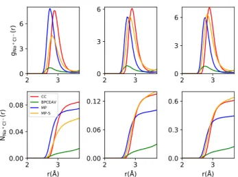
3.4. Ion-Pairing Effects.InFigure 4andTable 3, we have quantified the (Na+, Cl−) ion pairing as described by the different force fields. BPCEAV shows the smallest values for the RDF gNa+
Cl−(r) and the corresponding coordination numberNNa+Cl−(r) at the small Na+−Cl− distances (r < 4Å) considered here. This can be rationalized by the distance and well-depth parameters of the Lennard-Jones potentials, which are significantly different for BPCEAV compared with the other forcefields (see the Supporting Information). At larger
Figure 2.Concentration-dependent rescaled dielectric constantϵ*(c;
T) as defined byeq 13for NaCl solutions as obtained from our MD simulations with the CC forcefield (solid lines) and experiments60 (dashed lines) each at three different temperatures. The lines connecting the data points are only to guide the eye.
Figure 3. Dielectric constant ϵ at 300 K as a function of salt concentration as obtained from the MD simulations with the CC, BPCEAV, MP, and MPS forcefields (colored symbols) in comparison to the experimental data from60(black symbols). The indicated errors ϵobtained from the MD simulations have been obtained as described in the text. The solid lines (of same colors) are the result offittingeq 6to the corresponding data. Thefit parameters are compiled inTable 2.
Table 2. ParametersαandϵmsObtained by FittingEquation
6toϵ(c) from the MD Simulations with the Different Force Fields (See2.1) and the Experimental Data from Buchner et al.60,a
α(M−1) ϵ
ms ϵw ϵw−ϵms CC 13.9±0.4 18.9±1.3 71.5±1.9 52.6 BPCEAV 9.9±0.5 9.1±3.3 59.3±1.3 50.2 MP 11.1±0.4 17.4±1.4 59.3±1.3 41.9 MPS 9.3±0.5 21.8±2.1 59.3±1.3 37.5 expt. 11.7±0.3 28.8±2.1 78.3±1.3 49.5
aϵ
w=ϵ(c= 0 M) is obtained directly from the simulations for pure water or the experimental value,56respectively, and used to calculate the relative decrementϵw−ϵms.
distances, where the Coulomb interactions dominate, these differences are washed out. On the other hand, CC, MP, and MP-S show much stronger ion pairing, which may (partially) be responsible for the reduced dielectric decrement at high molarities. The question remains whether this is realistic or a shortcoming of the force fields used. Compared to ion association constants determined from conductometric meas-urements, our results clearly indicate too high probability of ion pairing. Fuoss61found an ion association constant ofKa= 0.82 for NaCl. Estimating the activity coefficients entering the equilibrium equation from a Davies expression, this would give ion association of below 1‰at 0.5 M concentration, much lower than what we observe. The strong ion association observed at 4 M would also suggest these ion pairs might be visible in X-ray diffraction measurements. No ion−ion contacts were, however, detected in X-ray diffraction measurements in 5 M solutions of NaCl.62Atfirst glance, the strong formation of contact ion pairs in CC, MP, and MP-S thus seems to be a shortcoming of these force fields. It may even indicate an incorrect solubility of NaCl in CC, MP, and MP-S. For the case of CC, a strongly reduced solubility compared with the experiment has actually been shown by Moučka et al.7(where CC is called SDGM). Reassuringly, however, although we observe a relatively high probability to form (Na+, Cl−) pairs, no excessively sharp peaks that could suggest formation of a
solid phase were observed in the Na+Na+ and Na+Cl− radial distribution functions even at high molarities.
To investigate this further, we compute ion association times from our MD simulations as described inSection 2.4.Figure 5
shows a histogram of these ion association times for the different force fields in a 3 M solution. The average pairing times for CC, BPCEAV, MP, and MP-S are 20, 3, 24, and 8 ps, respectively. This is on the same order of magnitude as the average pairing times observed by Rinne et al.30(12 ps) and still shorter than the decay times of 70 ps extracted by Sega et al.35from the dielectric response for the GROMOS forcefield. As shown by Sega et al.,35 long-lived ion pairs can significantly enhance the low-frequency dielectric response
χ(ω→0). On the other hand, Rinne et al.30found that pair formation times on the order of 12 ps do not spuriously enhance the low-frequency dielectric response. These authors also obtained reasonable agreement of their simulated dielectric response with experimental results, that is, χ(ω → 0) decreased with increasing molarity, as expected.
Even in the case that the ion association times in our simulations (especially for CC and MP) and the probability to form such an ion pair were sufficient to enhance the low-frequency dielectric response,χ, this would not show up in our calculations ofϵ.ϵ, as defined ineq 3, does not include ion-pairing effects, since the ion−ion and ion−water cross-terms are not considered. Since the effective field of the ion pair is reduced compared with that of an ion, ion pairing can therefore be expected to reduce the slope of ϵ(c) compared with a case without ion pairing. Our analysis hence suggests that the reduced slope of the dielectric constant as a function of concentration c observed for CC, MP, and MP-S at high concentrations, which is not in line with experimental results, may be due to the formation of spurious contact ion pairs.
3.5. Influence of Scaled Ionic Charges. As mentioned above, MP-S and BPCEAV result in a smaller ionic excess than CC and MP. It is immediately striking that the magnitude ofα seems to correlate with the ionic charge used in the forcefield. On average,αMP−S, BPCEAVis smaller thanαCC,MPby a factor of 0.77. Comparing onlyαMP−S and αMP, we find a factor 0.84. Considering the error bars inα, this compares reasonably well with the difference in ionic charges in the two groups of force
fields (qion=±0.85efor MP-S and BPCEAV andqion=±1efor CC and MP). To investigate this further, we plot the average
Figure 4. Radial distribution functions gNa+Cl−(r) (top row) and corresponding coordination numbers NNa+Cl−(r) (bottom row) calculated atc= 0.5 M (left column), 1.0 M (middle column), and 4.0 M (right column) using the four different forcefields.
Table 3. Value of the Coordination NumberNNa+Cl−(r= 3.4Å) Compared to the Probability of Ion Association Calculated Using a Value ofKa= 0.82 Determined by Fuoss61from Conductometric Measurements (Ion activities Were Estimated Using a Davies Expression)a
0.5 M 1.0 M 4 M
CC 0.074 0.12 0.586 BPCEAV 0.009 0.020 0.095 MP 0.069 0.111 0.519 MP-S 0.050 0.122 0.559 Expt.61 <0.001
MD30 ∼0.15
a
Finally, we also compare with the probability of contact ion pair formation obtained in molecular dynamics (MD) simulations by Rinne et al.30
Figure 5.Histogram of contact ion pair formation times for a 3 M solution. Note that all of the probability density functionspNapair+Cl−(t) are scaled to give a value of 1 at the shortest association times evaluated to allow for easier comparison of the different forcefields.
alignment of the water dipolesPNar +(r) andP Cl−
r (r) (around the
Na+and Cl−ions; seeeq 12) inFigure 6.
Naively, one would expect single water dipoles to align more strongly in thefield of more strongly charged ions andPr(r) to decrease asqion/r2, corresponding to the electricfield caused by the respective ion. This effect is, indeed, apparent inFigure 6
for the sodium ion at small distances below∼4 Å: Here, we observe a strong polarization near the ions that decreases rapidly as r increases. Furthermore, for r < 3 Å, the average polarization is clearly lower for MP-S and BPCEAV (both having charges scaled by 0.85) than for CC and MP (with chargesqion=±1e). As we go to larger distances around 4.8 Å, the average polarization increases again. This is likely caused by water−water interactions rather than direct water−ion interactions, which would also explain why there is no trend visible any more with the magnitude of qion in the different force fields. Interestingly, the second peak in the mean polarization does not correspond to the second solvation shell as indicated by the second maximum in the RDF but is shifted toward the tail of the second RDF peak.
For the chlorine ion, the situation becomes somewhat more complicated. At small distances below ∼3.6 Å, the average polarization is constant and does not increase above ∼0.6, independent of the forcefield used. A maximum value of 0.6 in average polarization around an anion may not come as a surprise, since this corresponds to the average polarization that we would expect if all water molecules point one H atom
toward the Cl−ion. That this value does not decrease up tor≈ 3.6Å likely indicates a saturation effect. This is indeed supported by the fact that the plateau region stops earlier for MP-S and BPCEAV (scaled charges) than for CC and MP and that the average polarization continues to lie lower for MP-S and BPCEAV than for CC and MP up tor≈4.3Å. As for Na+, we observe a second maximum in the average polarization at even larger distances (r≈ 5.7Å), which again corresponds to the (late) tail of the second solvation shell. We show in the
Supporting Informationthat this analysis (qualitatively) does
not change whenPClr −(r) is calculated based on the distance to
the closest hydrogen atom of the surrounding water molecules. To analyze this in even more detail, we will now concentrate on a comparison of the results for MP and MP-S only. Since these two forcefields differ only in the size of the ionic charges, their comparison allows us to directly extract the effect of the scaled charges without any influence of other force field parameters. From simple electrostatics, we would expect the average polarization to scale linearly with the chargeqionof the ion. We therefore present inFigure 7the results not only for
Pr; MPandPr; MP−Sbut also forPr; MP rescaled= 0.85·Pr; MP, which we might expect to lie on top ofPr; MP−S if the electrostatic ion−water dipole interaction is the only effect influencingPr. Indeed, at large distances, we observe a much better correlation between Pr; MP rescaled and Pr; MP−S than between Pr; MP and Pr; MP−S, suggesting that the pure electrostatic argument ofqionacting on the water dipoles holds. At smaller distances, however, deviations between the average polar-izationPr; MP rescaledandPr; MP−Sbecome apparent. For Cl−, we have already attributed this to saturation effects becoming important atr< 3.6 Å, that is, within thefirst solvation shell. The observed deviations for Na+ atr < 3.0 Å, that is, again
Figure 6.Average alignment of dipole vectorsPr(r) around Na+(top) and Cl−(bottom) ions. To allow a judgment on how likely it is tofind a dipole at distancer, we also plot the ion-oxygen RDF for the CC forcefield (gray line). The RDFs for the other forcefields are similar. Note that the results forPr(r) naturally become noisy at distances where the ion-oxygen RDF becomes small. All results are taken from 0.1 M solutions to avoid ion−ion interactions.
Figure 7.Same asFigure 6for MP and MP-S, but alsoPr; MP rescaled= 0.85·Pr; MPfor comparison.
within thefirst solvation shell, indicate that saturation effects also become important for the Na+ ion. This beginning saturation atr< 3.0 Å also explains why we do not observe a qualitative 1/r2behavior ofPr(r) at small distances.
This information should now be put together with the observations made forα, that is, thatαMP−S≈0.85αMP. Let us
first consider the case of Cl− in which Pr(r) within the first solvation shell is saturated independent of the forcefield and the ionic chargeqion used. Invoking the commonly accepted view of the dielectric decrement being caused on a single particle level by each independent water molecule orienting preferentially along the ionic field direction, the constant Pr would rather suggest a dielectric decrement that is independent of qion for the cases studied here. This is, however, not the case as seen by the change in α when changingqionin MP and MP-S. Our observation, which can (to a lesser extent) also be extended to the Na+ions, thus seems to back the idea put forward by Rinne et al.:30that the dielectric decrement is caused by an ion-induced breakdown of water− water interactions, which would show up to a much lesser extent inPr. Since the saturation effect inP
Na+
r is weaker than in
PClr −, it would be interesting to split the dielectric decrement
into a part stemming from the anions and one from the cations. This is, however, not easily achievable for neutral cells.
4. CONCLUSIONS
We have presented a comparative study of the performance of four different force fields for the description of the dielectric decrement observed at high ionic concentrations. Our focus was thereby not only to analyze the origin of the dielectric decrement in the different forcefields but also to investigate the influence of the scaling of ionic charges on the dielectric decrement.
For three of the forcefields studied, we found strong contact ion pair formation at high concentrations. For a 3 M solution, lifetimes between 8 and 24 ps were found. The strong contact ion pair formation in these force fields correlates with a reduced dielectric decrement at high concentrations, which is not in line with the experiment. We therefore argue that this strong ion pair formation is a result of an inaccurate description of interactions in those forcefields.
The influence of scaling of ionic charges was investigated at low concentrations. Our analysis of the dielectric decrement suggests a close to 1:1 relation between the ionic charge and the initial slope of the dielectric constant as a function of concentration. While this may be expected, it seems to be at odds with the average polarization Pr(r) of water molecules around an ion. Within the first solvation shell, where polarization effects are the strongest, we found a negligible influence of the ion charge onPr(r) around Cl−. Around Na+, the polarization did depend on the ion charge, but the scaling was not linear. Only at larger distances, a linear scaling ofPr(r) with the ion charge was found. If the ionic decrement were thus a pure saturation effect, we would not expect the dielectric decrement to scale linearly with ionic charge. This observation strengthens the argument put forward by Rinne et al.,30who suggested that the dielectric decrement may be caused by an ion-induced disturbance of the water−water correlations, which causes a reduction of the Kirkwood g factor and hence of the dielectric constant, rather than by a saturation effect in the water alignment.
■
ASSOCIATED CONTENT*
S Supporting InformationThe Supporting Information is available free of charge on the
ACS Publications websiteat DOI:10.1021/acs.jpcb.9b07916.
Force field parameters: well-depth parameters of Lennard-Jones potentials, distance parameters of Len-nard-Jones potentials, charges of hydrogen and oxygen atoms as well as sodium and chloride ions used in the different forcefield parameter sets; average dipole vector alignment around the Cl−ion (PDF)
■
AUTHOR INFORMATIONCorresponding Author
*E-mail: j.meyer@chem.leidenuniv.nl. Phone: +31 (0)71 527 5569
ORCID
Katharina Doblhoff-Dier:0000-0002-5981-9438
Jörg Meyer:0000-0003-0146-730X
Author Contributions
†S.S. and K.D.-D. contributed equally to this work.
Notes
The authors declare no competingfinancial interest.
■
ACKNOWLEDGMENTSJ.M. gratefully acknowledges financial support from The Netherlands Organisation for Scientific Research (NWO) under Vidi Grant no. 723.014.009.
■
REFERENCES(1) Mathew, K.; Sundararaman, R.; Letchworth-Weaver, K.; Arias, T. A.; Hennig, R. G. Implicit Solvation Model for Density-Functional Study of Nanocrystal Surfaces and Reaction Pathways.J. Chem. Phys.
2014,140, No. 084106.
(2) Fisicaro, G.; Genovese, L.; Andreussi, O.; Marzari, N.; Goedecker, S. A Generalized Poisson and Poisson-Boltzmann Solver for Electrostatic Environments.J. Chem. Phys.2016,144, No. 014103. (3) Dupont, C.; Andreussi, O.; Marzari, N. Self-Consistent Continuum Solvation (SCCS): The Case of Charged Systems. J. Chem. Phys.2013,139, No. 214110.
(4) Sundararaman, R.; Letchworth-Weaver, K.; Schwarz, K. A. Improving Accuracy of Electrochemical Capacitance and Solvation Energetics in First-Principles Calculations.J. Chem. Phys.2018,148, No. 144105.
(5) Hörmann, N. G.; Andreussi, O.; Marzari, N. Grand Canonical Simulations of Electrochemical Interfaces in Implicit Solvation Models.J. Chem. Phys.2019,150, No. 041730.
(6) Valiskó, M.; Boda, D. The Effect of Concentration- and Temperature-Dependent Dielectric Constant on the Activity Coefficient of NaCl Electrolyte Solutions.J. Chem. Phys.2014,140, No. 234508.
(7) Moučka, F.; Nezbeda, I.; Smith, W. R. Molecular Force Fields for Aqueous Electrolytes: SPC/E-Compatible Charged LJ Sphere Models and Their Limitations.J. Chem. Phys.2013,138, No. 154102. (8) Nezbeda, I.; Moucka, F.; Smith, W. R. Recent Progress iň Molecular Simulation of Aqueous Electrolytes: Force Fields, Chemical Potentials and Solubility.Mol. Phys.2016,114, 1665−1690. (9) Smith, W. R.; Nezbeda, I.; Kolafa, J.; Moucka, F. Recent Progresš in the Molecular Simulation of Thermodynamic Properties of Aqueous Electrolyte Solutions.Fluid Phase Equilib.2018,466, 19−30. (10) Kann, Z. R.; Skinner, J. L. A Scaled-Ionic-Charge Simulation Model That Reproduces Enhanced and Suppressed Water Diffusion in Aqueous Salt Solutions.J. Chem. Phys.2014,141, No. 104507.
(11) Leontyev, I. V.; Stuchebrukhov, A. A. Electronic Continuum Model for Molecular Dynamics Simulations.J. Chem. Phys.2009,130, No. 085102.
(12) Leontyev, I.; Stuchebrukhov, A. Accounting for Electronic Polarization in Non-Polarizable Force Fields.Phys. Chem. Chem. Phys.
2011,13, 2613−2626.
(13) Mason, P. E.; Wernersson, E.; Jungwirth, P. Accurate Description of Aqueous Carbonate Ions: An Effective Polarization Model Verified by Neutron Scattering.J. Phys. Chem. B2012,116, 8145−8153.
(14) Li, P.; Merz, K. M. Metal Ion Modeling Using Classical Mechanics.Chem. Rev.2017,117, 1564−1686.
(15) Wendler, K.; Dommert, F.; Zhao, Y. Y.; Berger, R.; Holm, C.; Site, L. D. Ionic Liquids Studied across Different Scales: A Computational Perspective.Faraday Discuss.2011,154, 111−132.
(16) Pegado, L.; Marsalek, O.; Jungwirth, P.; Wernersson, E. Solvation and Ion-Pairing Properties of the Aqueous Sulfate Anion: Explicit versus Effective Electronic Polarization. Phys. Chem. Chem. Phys.2012,14, 10248−10257.
(17) Benavides, A. L.; Portillo, M. A.; Chamorro, V. C.; Espinosa, J. R.; Abascal, J. L. F.; Vega, C. A Potential Model for Sodium Chloride Solutions Based on the TIP4P/2005 Water Model. J. Chem. Phys.
2017,147, No. 104501.
(18) Blüh, O. Die Dielektrizitätskonstanten von Elektrolytlösungen.
Z. Phys.1924,25, 220−229.
(19) Hasted, J. B.; Ritson, D. M.; Collie, C. H. Dielectric Properties of Aqueous Ionic Solutions. Parts I and II.J. Chem. Phys.1948,16, 1− 21.
(20) Haggis, G. H.; Hasted, J. B.; Buchanan, T. J. The Dielectric Properties of Water in Solutions.J. Chem. Phys.1952,20, 1452−1465. (21) Glueckauf, E. Bulk Dielectric Constant of Aqueous Electrolyte Solutions.Trans. Faraday Soc.1964,60, 1637−1645.
(22) Liszi, J.; Felinger, A.; Kristóf, E. H. Static Relative Permittivity of Electrolyte Solutions.Electrochim. Acta1988,33, 1191−1194.
(23) Adar, R. M.; Markovich, T.; Levy, A.; Orland, H.; Andelman, D. Dielectric Constant of Ionic Solutions: Combined Effects of Correlations and Excluded Volume. J. Chem. Phys. 2018, 149, No. 054504.
(24) Gavish, N.; Promislow, K. Dependence of the Dielectric Constant of Electrolyte Solutions on Ionic Concentration: A Microfield Approach.Phys. Rev. E2016,94, No. 012611.
(25) Persson, R. A. X. On the Dielectric Decrement of Electrolyte Solutions: A Dressed-Ion Theory Analysis.Phys. Chem. Chem. Phys.
2017,19, 1982−1987.
(26) Kjellander, R. Focus Article: Oscillatory and Long-Range Monotonic Exponential Decays of Electrostatic Interactions in Ionic Liquids and Other Electrolytes: The Significance of Dielectric Permittivity and Renormalized Charges. J. Chem. Phys. 2018, 148, No. 193701.
(27) Levy, A.; Andelman, D.; Orland, H. Dielectric Constant of Ionic Solutions: A Field-Theory Approach.Phys. Rev. Lett.2012,108, No. 227801.
(28) Adar, R. M.; Markovich, T.; Andelman, D. Bjerrum Pairs in Ionic Solutions: A Poisson-Boltzmann Approach.J. Chem. Phys.2017,
146, No. 194904.
(29) Demery, V.; Dean, D. S.; Podgornik, R. Electrostatić Interactions Mediated by Polarizable Counterions: Weak and Strong Coupling Limits.J. Chem. Phys.2012,137, No. 174903.
(30) Rinne, K. F.; Gekle, S.; Netz, R. R. Dissecting Ion-Specific Dielectric Spectra of Sodium-Halide Solutions into Solvation Water and Ionic Contributions.J. Chem. Phys.2014,141, No. 214502.
(31) Kirkwood, J. G. The Dielectric Polarization of Polar Liquids.J. Chem. Phys.1939,7, 911−919.
(32) Anderson, J.; Ullo, J.; Yip, S. Molecular Dynamics Simulation of the Concentration-Dependent Dielectric Constants of Aqueous Nacl Solutions.Chem. Phys. Lett.1988,152, 447−452.
(33) Chowdhuri, S.; Chandra, A. Molecular Dynamics Simulations of Aqueous NaCl and KCl Solutions: Effects of Ion Concentration on
the Single-Particle, Pair, and Collective Dynamical Properties of Ions and Water Molecules.J. Chem. Phys.2001,115, 3732−3741.
(34) Sala, J.; Guardia, E.; Martí, J. Effects of Concentration oǹ Structure, Dielectric, and Dynamic Properties of Aqueous NaCl Solutions Using a Polarizable Model. J. Chem. Phys. 2010, 132, No. 214505.
(35) Sega, M.; Kantorovich, S. S.; Holm, C.; Arnold, A. Communication: Kinetic and Pairing Contributions in the Dielectric Spectra of Electrolyte Solutions. J. Chem. Phys. 2014, 140, No. 211101.
(36) Pache, D.; Schmid, R. Molecular Dynamics Investigation of the Dielectric Decrement of Ion Solutions. ChemElectroChem 2018, 5, 1444−1450.
(37) Zasetsky, A. Y.; Svishchev, I. M. Dielectric Response of Concentrated NaCl Aqueous Solutions: Molecular Dynamics Simulations.J. Chem. Phys.2001,115, 1448−1454.
(38) Fuentes-Azcatl, R.; Barbosa, M. C. Sodium Chloride, NaCl/ϵ: New Force Field.J. Phys. Chem. B2016,120, 2460−2470.
(39) Smith, D. E.; Dang, L. X. Computer Simulations of NaCl Association in Polarizable Water.J. Chem. Phys. 1994,100, 3757− 3766.
(40) Berendsen, H. J. C.; Grigera, J. R.; Straatsma, T. P. The Missing Term in Effective Pair Potentials.J. Phys. Chem. A1987,91, 6269− 6271.
(41) Mao, A. H.; Pappu, R. V. Crystal Lattice Properties Fully Determine Short-Range Interaction Parameters for Alkali and Halide Ions.J. Chem. Phys.2012,137, No. 064104.
(42) Abascal, J. L. F.; Vega, C. A General Purpose Model for the Condensed Phases of Water: TIP4P/2005.J. Chem. Phys.2005,123, No. 234505.
(43) Plimpton, S. Fast Parallel Algorithms for Short-Range Molecular Dynamics. J. Comput. Phys. 1995, 117, 1−19.
DOI: 10.1006/jcph.1995.1039.
(44) Martínez, L.; Andrade, R.; Birgin, E. G.; Martínez, J. M. PACKMOL: A Package for Building Initial Configurations for Molecular Dynamics Simulations. J. Comput. Chem. 2009, 30, 2157−2164.DOI: 10.1002/jcc.21224.
(45) Berendsen, H. J. C.; Postma, J. P. M.; van Gunsteren, W. F.; DiNola, A.; Haak, J. R. Molecular Dynamics with Coupling to an External Bath.J. Chem. Phys.1984,81, 3684−3690.
(46) Nosé, S. A Unified Formulation of the Constant Temperature Molecular Dynamics Methods.J. Chem. Phys.1984,81, 511−519.
(47) Hoover, W. G. Canonical Dynamics: Equilibrium Phase-Space Distributions.Phys. Rev. A1985,31, 1695−1697.
(48) in’t Veld, P. J.; Ismail, A. E.; Grest, G. S. Application of Ewald Summations to Long-Range Dispersion Forces.J. Chem. Phys.2007,
127, No. 144711.
(49) Hockney, R. W.; Eastwood, J. W.Computer Simulation Using Particles; Adam Hilger: NY, 1989.
(50) Neumann, M.; Steinhauser, O.; Pawley, G. S. Consistent Calculation of the Static and Frequency-Dependent Dielectric Constant in Computer Simulations.Mol. Phys.1984,52, 97−113.
(51) Caillol, J. M.; Levesque, D.; Weis, J. J. Theoretical Calculation of Ionic Solution Properties.J. Chem. Phys.1986,85, 6645−6657.
(52) Sega, M.; Kantorovich, S.; Arnold, A. Kinetic Dielectric Decrement Revisited: Phenomenology of Finite Ion Concentrations.
Phys. Chem. Chem. Phys.2015,17, 130−133.
(53) Flyvbjerg, H.; Petersen, H. G. Error Estimates on Averages of Correlated Data.J. Chem. Phys.1989,91, 461−466.
(54) Spencer, J. Pyblock. Software available from https://github. com/jsspencer/pyblock(accessed Aug 13, 2019).
(55) Lee, R. M.; Conduit, G. J.; Nemec, N.; López Ríos, P.; Drummond, N. D. Strategies for Improving the Efficiency of Quantum Monte Carlo Calculations. Phys. Rev. E 2011, 83, No. 066706.
(56) Barthel, J.; Bachhuber, K.; Buchner, R.; Hetzenauer, H. Dielectric Spectra of Some Common Solvents in the Microwave Region. Water and Lower Alcohols.Chem. Phys. Lett.1990,165, 369− 373.
(57) Gereben, O.; Pusztai, L. On the Accurate Calculation of the Dielectric Constant from Molecular Dynamics Simulations: The Case of SPC/E and SWM4-DP Water.Chem. Phys. Lett.2011,507, 80−83. (58) Elton, D. C. Understanding the Dielectric Properties of Water. Ph.D. Thesis, Stony Brook University, New York, 2016.
(59) Kusalik, P. G.; Svishchev, I. M. The Spatial Structure in Liquid Water.Science1994,265, 1219−1221.
(60) Buchner, R.; Hefter, G. T.; May, P. M. Dielectric Relaxation of Aqueous NaCl Solutions.J. Phys. Chem. A1999,103, 1−9.
(61) Fuoss, R. M. Conductimetric Determination of Thermody-namic Pairing Constants for Symmetrical Electrolytes. Proc. Natl. Acad. Sci. USA1980,77, 34−38.
(62) Marcus, Y.; Hefter, G. Ion Pairing. Chem. Rev. 2006, 106, 4585−4621.