Stability and fluctuations in black hole thermodynamics
George Ruppeiner*Division of Natural Sciences, New College of Florida, 5800 Bay Shore Road, Sarasota, Florida 34243-2109, USA
(Received 12 December 2006; published 26 January 2007)
I examine thermodynamic fluctuations for a Kerr-Newman black hole in an extensive, infinite environment. This problem is not strictly solvable because full equilibrium with such an environment cannot be achieved by any black hole with massM, angular momentumJ, and chargeQ. However, if we consider one (or two) ofM,J, orQto vary so slowly compared with the others that we can regard it as fixed, instances of stability occur, and thermodynamic fluctuation theory could plausibly apply. I examine seven cases with one, two, or three independent fluctuating variables. No knowledge about the thermody-namic behavior of the environment is needed. The thermodythermody-namics of the black hole is sufficient. Let the fluctuation moment for a thermodynamic quantityXbephX2i. Fluctuations at fixedMare stable for all thermodynamic states, including that of a nonrotating and uncharged environment, corresponding to average valuesJQ0. Here, the fluctuation moments forJandQtake on maximum values. That for Jis proportional toM. For the Planck mass it is0:3990@. That forQis3:301e, independent ofM. In all cases, fluctuation moments forM,J, and Q go to zero at the limit of the physical regime, where the temperature goes to zero. WithMfluctuating there are no stable cases for averageJQ0. But, there are transitions to stability marked by infinite fluctuations. For purelyMfluctuations, this coincides with a curve which Davies identified as a phase transition.
DOI:10.1103/PhysRevD.75.024037 PACS numbers: 04.70.Dy, 05.40.a, 05.70.a
I. INTRODUCTION
The fundamental simplicity of black holes has led to their thermodynamic description [1–3]. Viewed from out-side, Kerr-Newman black holes can be characterized only by their mass M, angular momentum J, and charge Q. Detailed internal structure and history of formation are irrelevant in this ‘‘no hair’’ property. Such a drastic reduc-tion of complexity is characteristic of thermodynamic systems.
In this description, black hole entropy is proportional to the area of the event horizon. With the appropriate multi-plier, this entropy may be added to the entropy of any conventional thermodynamic system. The sum obeys a generalized second law of thermodynamics, with nonde-creasing total entropy for a closed composite system.
But entropy is also connected to microscopic informa-tion (number of accessible microstates), raising the possi-bility of a thermodynamic fluctuation theory [4] based on Einstein’s formula for the probability,
P/expStot=kB; (1) where Stot is the entropy of the closed system and kB is Boltzmann’s constant. While the nature of such informa-tion probably requires a future quantum theory of gravity, the thermodynamic formalism allows us to proceed know-ing just the entropy.
Strictly speaking, a thermodynamic fluctuation ap-proach is unviable since a Kerr-Newman black hole cannot come to equilibrium with any extensive, infinite environ-ment. For no physical values of M, J, or Q is the full
Hessian determinant1 of the black hole entropy S
SM; J; Q negative definite [5], as it must be to produce a local maximum in the total entropy. This puts the full problem, withM; J; Qall fluctuating, beyond the reach of the standard thermodynamic fluctuation formalism. Dynamically, physics ultimately favors extreme situations where the black hole either evaporates completely or grows without limit.
In reality, however, one of the variablesM,J, orQmay be slow to change in time compared with the other two. Physically, it would be surprising if they all went at the same rate. This possibility offers the restricted class of problems with just two fluctuating variables, and the third effectively fixed or drifting very slowly out of equilibrium with the environment. There is also the possibility of a single fluctuating variable, with the other two fixed.
In this paper I consider all seven possible cases: fluctu-atingM; J; Q,J; Q,M; Q,M; J,M,J, andQ. Seven entropy Hessian determinants:p1,p2,p3,p01,p02,p002, and
p001, in various combinations, govern fluctuations. For stability, the relevant Hessian determinants must all be positive. As we will see, p3 is always negative, p01, p
0
2, andp001 are never negative, andp1, p2, andp002 may have either sign depending on the thermodynamic state. This means that the fluctuation case M; J; Qis not stable for any thermodynamic state,J; Q,J, andQare stable for all states, andM; J,M; Q, andMmay be stable or unstable depending on the thermodynamic state.
*Electronic address: [email protected]
1By Hessian determinant I mean a determinant of a square
This paper is arranged as follows. First, I summarize the basic thermodynamic fluctuation formalism as it applies to black holes. Second, I give a stability and fluctuation analysis of all seven cases above. Third, I discuss which cases might be physically relevant.
II. THERMODYNAMIC FLUCTUATION THEORY
A. Black hole thermodynamics
General relativity, including thermodynamic arguments, allows one to calculate the Kerr-Newman black hole en-tropy [3,6]
SM; J; Q 1
82M
2Q22qM4J2M2Q2: (2)
HereM,J, andQare expressed in length units,MandQin cm, andJ in cm2. To convert to ‘‘real’’ units (Qin esu) write: M c2 G ; J c3 G
; and Q
c2
G1=2
; (3)
whereGis the constant of gravity andcis the speed of light [7]. In these geometrized units,Gc1.
To convert S to real units requires more discussion. Bekenstein [1] and Hawking [2] gave the conventional unit black hole entropySbh,2
Sbh kB 1 4 A L2 p ; (4)
whereAis the black hole area [6],
A42M2Q22qM4J2M2Q2; (5)
Lpis the Planck length,
Lp @G c3 s
1:6161033 cm; (6)
and@is Planck’s constant divided by2.3This leads to the conversion factor forS,
Sbh kB
S
8
L2p
: (7)
As emphasized by Bekenstein [1], a theory containing both @andGhas a quantum gravity flavor.4
The quantitiesM,J, andQare conserved. This makes them natural coordinates for treating the interaction be-tween two thermodynamic systems.
Entropy, though additive between two systems, is not conserved. Neither is black hole entropy extensive. That is, if M, J, and Q are scaled up by a common factor, the entropy does not scale up by the same factor.
Define the black hole temperatureT(proportional to the constant surface gravity), the angular velocity , and the constant surface electric potentialby [3,5]
1 T @S @M J;Q ; (8) T @S @J M;Q ; (9) and T @S @Q M;J : (10)
Equations (2) and (8) yield
1
T M
4
2 2
1
p
; (11)
where the positive dimensionless quantities
J
2
M4; (12)
and
Q
2
M2: (13)
RealTandSrequire
<1: (14)
Equality in Eq. (14) would clearly have T !0, which violates the third law of black hole thermodynamics for-bidding naked singularities [9]. I refer to conditions sat-isfying Eq. (14) as the physical regime.
SM; J; Qis a homogeneous function of the variables
M;pJ; Q [6]. I shall use the term special homogeneous function (SHF) for a function of the form
Maf; ; (15)
where the constant aand the functionf; are dimen-sionless.Sis an SHF since, by Eq. (2),
S1 8M
222p1: (16) It is straightforward to prove: (1) if a function is an SHF, then its derivative with respect to any ofM,J, orQis an SHF, (2) multiplying and dividing two SHF’s results in an SHF, and (3) adding or subtracting two SHF’s results in an SHF. The last follows since addition or subtraction requires the SHF’s to have the same units, and hence the same value ofa. Since we may construct all the thermodynamic func-tions in this paper with the operafunc-tions above starting with
SM; J; Q, they must all be SHF’s. Hence, we may
repre-2Bekenstein first gave this in his Eq. (17), page 2338, but with
a prefactor other than1
4. Hawking corrected this on his page 193.
3Thus, entropy in units ofk
Bis 1=4the Area in units of the
Planck area; see [8] for a recent semipopular discussion.
4The entropy in this paper is the same as that of Davies [3],
sent the signs of our seven Hessian determinants with just two variables, rather than the three we might expect.
B. Black hole fluctuations
Consider now the environment surrounding the black hole. I regard it to be an extensive, infinite thermodynamic system of particles and photons with entropy Se. As dis-cussed by Hawking [2], forfinite environments scenarios of full equilibrium with a single black hole exist. Pavo´n and Rubı´ [10] have worked out a thermodynamic fluctuation theory for such a case. Katz, Okamoto, and Kaburaki [11] have also analyzed stability for a number of ensembles involving Kerr-Newman black holes. But theories based on finite environments depend as well on the thermodynamics of the environment, which might not be known. By con-trast, the more physically relevant extensive, infinite envi-ronments result in fluctuation expressions dependent only on the known thermodynamic properties of the black hole.
The total entropy
StotSSe (17)
obeys a generalized second law of thermodynamics that for a closed system it not decrease [1–3]. I will build the thermodynamic fluctuation theory around the Gaussian expansion ofStot[4].
Introduce the notation [12]
X1; X2; X3 M; J; Q; (18) and
F
@S
@X; (19)
with corresponding properties of the environment denoted by the subscripte. Let us assume (incorrectly, as we will see) that the black hole and the environment are fully in equilibrium, with a local maximum for Stot. Consider a small fluctuation X away from this equilibrium. To second order,
StotFXFeXe
1 2
@F @XX
X
1
2
@Fe
@X e
XeXe; (20)
where the coefficients are evaluated at the equilibrium state, which is set by the environment. The conservation laws demand
X Xe; (21)
and a necessary condition for maximum entropy is
FFe: (22)
If the environment is very large, the second quadratic term in Eq. (20) is negligible compare with the first. To see this, fix the values ofXe. As the extensive environment is scaled up to infinity at fixed Fe, Xe scales up without
limit, and @Fe=@Xe!0. The ability to drop this qua-dratic term is a significant simplification offered by an infinite environment.
Equation (20) now becomes
Stot 12gXX; (23)
where the symmetric matrix
g
@2S
@X@X: (24)
An essential point in this paper is that if we set one or two Xto zero, the sum Eq. (23) is only trivially modified. The corresponding F’s need not be set equal as in Eq. (22). Entropy maximum requires that the matrixg
of the remaining variable(s) be positive definite. Conditions under which this might be satisfied are dis-cussed in Sec. III.
The Gaussian approximation to the thermodynamic fluc-tuation theory results from Eqs. (1), (7), and (23) [4]. The probability (written for n3 variables) of finding the thermodynamic state in the range X1; X2; X3 to (X1
dX1,X2dX2,X3dX3) is
PdX1dX2dX3
p
2n=2 exp
1
2X
X
dX1dX2dX3; (25)
where
8
L2 p
g; (26)
andis the determinant of. The modification ifn <3 is obvious.
All first fluctuation moments are zero [4]:
hXi 0: (27)
Second fluctuation moments are
hXXi ; (28)
withthe components of the inverse
matrix.
C. Black hole phase transitions
Discussed have been possible phase transitions associ-ated with black holes [3]; see Refs. [13,14] for recent references. In regular thermodynamic systems, phase tran-sitions are usually presented in the context of microscopic properties coupling to macroscopic thermodynamics [15]. Such an approach is not yet possible with black holes. Although there is a thermodynamic picture, the micro-scopic picture is mostly missing. This considerably com-plicates the discussion.
easy to construct thermodynamic quantities which diverge for any state.5Perhaps, by analogy with fluid systems, the divergence of quantities such as heat capacities has some special status. But, in the absence of microscopic models, it is hard to be sure.
Interesting are discussions of phase transitions with some change of black hole topology [13,14]. But Kerr-Newman black holes have a spherical topology in the physical regime. Some authors draw conclusions from scaling relations among critical exponents [16]. The diver-gence of the curvature in a geometric approach to thermo-dynamics has also been connected to black hole phase transitions [13,14,17,18]. In this paper I add the divergence in second fluctuation moments of conserved quantities to the discussion. But, other than to suggest this, I draw no particular conclusions with respect to phase transitions.
III. SEVEN FLUCTUATION CASES
In this section, I analyze the seven possible fluctuation cases. The discussion is mostly formal, with considerations of physical significance deferred to the next section.
In reading difficult thermodynamic calculations, one can easily lose perspective in following simplification tricks. To avoid this, I work directly inM,J, andQcoordinates and use Mathematica to perform the computational tedium. Since stability and fluctuations are independent of the coordinates used to calculate them, we need never fear missing something essential by working in the ‘‘wrong’’ coordinates. The necessary quantities of analysis are the seven Hessian determinantsp1,p2,p3,p10,p02,p002, andp001
defined below. These are all SHF’s, so I can represent their signs simply by finding their dependence onJandQ.
First, some general remarks about my results. All second fluctuation moments involving M, J, or Q in the stable regime go to zero at the limit of the physical regime (
1). All cases involving fluctuations at fixed M are stable for all thermodynamic states. This includes physi-cally perhaps the most important state with average J
Q0, corresponding to a nonrotating, uncharged environ-ment. No case with fluctuatingM is stable for this state. The switch from unstable to stable is accompanied by an infinity inphM2i. For purelyMfluctuations, this tran-sition occurs at the Davies phase trantran-sition point.
A.M; J; Qfluctuating
Here, all threeM; J; Qfluctuate and relevant is the full second order expansion forStot, Eq. (23). Necessary and sufficient conditions [19] that the quadratic form for
Stotbe positive definite is that
p1g11>0; (29)
p2
g11 g12
g21 g22
>0; (30) and
p3
g11 g12 g13
g21 g22 g23
g31 g32 g33
>0: (31)
Consider first p3. Direct evaluation of Eq. (31), using Eqs. (2) and (24), shows
p3
K43K33K23L2K2KL45L24
64M2K5 ;
(32)
where the combination of variables [5]:
Kp1; (33)
and
Lp1: (34)
Figure1showsM2p
3. The values displayed are all nega-tive. Indeed, Tranah and Landsberg [5] proved thatp3<0 for all states in the physical regime, violating the inequality Eq. (31). There are thus no stable cases with M; J; Qall fluctuating. Figure2show this schematically.
Note also that p3 diverges at the limit of the physical regime, K!0, as do all of the Hessian determinants in this section.
B.J; Qfluctuating,Mfixed
Here,J; Qfluctuate at fixedM. By Eq. (23),
2Stotg22J22g23JQg33Q2: (35)
By Eq. (20), fixing the masses means that the temperatures of the black hole and the environment need not match. FIG. 1. M2p
3 as a function of J=M2 for several values of Q=M.p3is negative for all values shown. The curves all diverge at the end of the physical regime1.
5For example, iff is a regular thermodynamic function with
Maximum entropy in the equilibrium state requires
p01g22>0; (36) and
p02
g22 g23
g32 g33
>0: (37) Direct calculation shows
p01 K
2L21
4M2K3 ; (38)
and
p02 K
3 L21K1
16M2K4 : (39)
SinceK0andL1, we see thatp01 andp02 are never negative in the physical regime, and fluctuations are stable. Figure3shows this schematically.
Physically, the environment most easily realized is non-rotating and uncharged. This corresponds to average values
JQ0. Here, direct calculation with Eq. (28) yields the fluctuation moments shown in TableI. Fluctuations inJ
scale up directly withM. At the Planck mass
Mp
@c G
s
2:177105 g1:6161033 cm;
(40)
Jfluctuates at a little less than [email protected] inQare independent of M, a little more than three fundamental charges.
Table I also shows the fluctuation moments along the axesJ0andQ0. For givenK, the mass dependence
is the same as for the origin. Along each coordinate axis, fluctuation moments for bothJandQare maximum at the origin, and decrease monotonically to zero at the end of the physical regime.
C.M; Qfluctuating,Jfixed
Here,M; Qfluctuate at fixedJ. By Eq. (23),
2Stotg11M22g13MQg33Q2:
(41) FIG. 3. Stable fluctuation regime forJ; Qfluctuating at fixed M. The plus signs indicate the signs of bothp01andp02. Clearly, Stot may have a local maximum at any point in the physical regime.
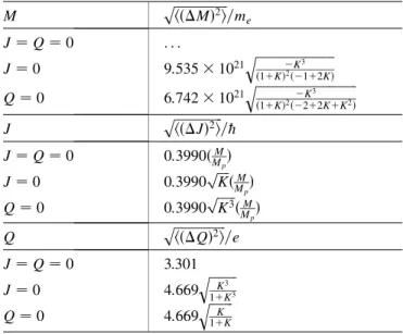
TABLE I. Fluctuation moments for stable fluctuations at the origin and along the axes ofJ,Qspace for (top to bottom)J; Q, M; Q, and M; J fluctuations. Unstable cases are indicated with a ‘‘. . ..’’ In all the stable cases on the coordinate axes, off diagonal elements, e.g.hMJi, are zero.
J; Q phJ2i=@ phQ2i=e
JQ0 0:3990M
Mp 3.301
J0 0:3990pKM
Mp 4:669
K3
1K31=2
Q0 0:3990pK3M
Mp 4:669
K
1K
1=2
M; Q phM2i=m
e
hQ2i p
=e
JQ0 . . . .
J0 . . . .
Q0 6:7421021 K3
1K22KK2 q
4:669 K
1K
1=2
M; J phM2i=m
e
hJ2i p
=@
JQ0 . . . .
J0 9:5351021 K3
1K212K q
0:3990pKM Mp
Q0 . . . .
FIG. 2. Fluctuation regimes forM; J; Qall free to fluctuate. The curve marks the end of the physical regime1. The minus signs (signs ofp3) indicate thatStothas no local maximum anywhere in the physical regime.
6For a Planck mass black hole, the entropy in Eq. (7), and
therefore the number of microstates, is of order unity. It is hard to imagine the character of a black hole with a smaller mass.
By Eq. (20), fixingJmeans that the angular velocities of the black hole and its environment need not match. Stability requires
p1>0; (42)
and
p002
g11 g13
g31 g33
>0: (43) Direct calculation shows
p1 2KL
2K22KL2
4K3 ; (44)
and
p002 K
4 L24K3 L22K2 L42L24K2L45L24
16K4 : (45)
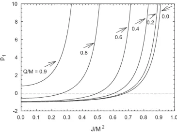
Figure4showsp1. It has regimes of positive and nega-tive values separated by a curve of zeros which follows from setting the numerator in Eq. (44) to zero. The only solution in the physical regime is2KL2, which may be written
2643: (46) As emphasized by Davies [3], Eq. (46) marks a diverging heat capacity
CJ;QT @S
@T
J;Q
: (47)
This connects top1via7
p1 1
T2C J;Q
: (48)
Figure 5showsp002, which has regimes of positive and negative values separated by a curve of zeros.8Fig.6shows this curve as well as the curvep1 0. Also shown is the regime of stable fluctuations where both p1 and p002 are positive. Clearly, the only coordinate axis in J, Q space with stable fluctuations is the J axis. Table I shows the stableM; Qfluctuation moments forQ0, withmethe electron mass. Fluctuations in M start unstable at the origin, but become stable when K exceeds 0.7321 (J=M20:6813).
FIG. 4. p1as a function ofJ=M2for several values ofQ=M.p1 may be positive or negative. The curves all diverge at the end of the physical regime.
FIG. 5. p002 as a function ofJ=M2for several values ofQ=M. p002may be positive or negative. The curves all diverge at the end of the physical regime.
7There is a minor typographical error in Ref. [5]. On the right
hand side of Eq. (3.17),Cshould beL.
For givenK, neither fluctuation moment depends onM. Fluctuations in M expressed in electron units are huge, requiring many electron masses to produce a sizable change in Stot. In contrast, very few electron charges are required to vary Q by its fluctuation moment. This pattern is more general, and leads me in the next section to consider mass as a drifting parameter not governed by the statistics of thermodynamic fluctuations.9
All the fluctuation moments diverge along the curve
p002 0 because on inverting the coefficient matrix in Eq. (41) p002 goes on the bottom. There are no anomalies in the fluctuation moments along the Davies infinity curve
p10, which is not in the stable regime.
D.M; Jfluctuating,Qfixed
Here,M; Jfluctuate at fixedQ. By Eq. (23),
2Stotg11M22g12MJg22J2: (49)
By Eq. (20), fixingQmeans that the potentials of the black hole and its environment need not match.
Stability requires
p1>0; (50) and
p2>0: (51) Direct calculation shows
p2 2K
33K22L21K3L24
16M2K4 : (52)
Figure7showsM2p
2. It has both positive and negative values.p2is zero10in the physical regime if and only if
34
2
412 : (53)
This curve of zeros is shown in Fig.8, along with that for
p1. There is a regime in the physical region where bothp1
andp2 are positive and fluctuations are stable.
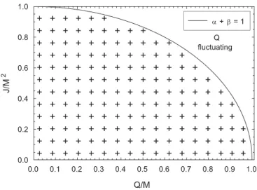
From Fig. 8, the only coordinate axis with stable fluc-tuations is the Q axis. Table I shows the stable M; J
fluctuation moments. Fluctuations start unstable at the origin, but for J0become stable atK1=2(Q=M 0:8660). This stable regime corresponds to the black hole FIG. 7. M2p
2 as a function of J=M2 for several values of Q=M. p2 may be positive or negative. The curves all diverge at the end of the physical regime.
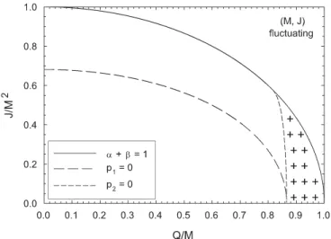
FIG. 6. Stable fluctuation regime for M; Qat fixed J. The physical regime wherep1andp002 are both positive is indicated bysigns.
FIG. 8. Stable fluctuation regime forM; Jfluctuating at fixed Q. The physical regime where p1 and p2 are both positive is indicated bysigns.
9However, if the charged entities producing fluctuations were
predominantly, say, quantum black holes with the Planck mass, and we substituted Mp for me in Table I, the multiplier for
hM2i p
=Mp would be the far more reasonable 0.3990.
10This curve of zeroes corresponds to diverging C
;Q in
in a nonrotating environment. For givenK, the fluctuation moment forMis mass independent while that forJscales up in proportion to mass.
Off the coordinate axes, the fluctuation moments all diverge along the curvep2 0, sincep2is the determinant of the coefficients in Eq. (49). There are no anomalies in the fluctuation moments along the Davies curve p10, which is not in the stable regime.
E.Mfluctuating,J,Qfixed
Here,Mfluctuates at fixedJandQ. By Eq. (23),
2Stotg11M2: (54)
Stability requires
p1>0: (55) Figure 9 shows the regime of stable fluctuations. The origin is unstable, but each coordinate axis has a stable regime, shown in TableII. Fluctuations inMbecome stable along theQaxis atK1=2(Q=M0:8660), and along theJaxis atK0:7321(J=M20:6813). For givenK, the fluctuation moment forMis mass independent.
Off the coordinate axes, the M fluctuation moment diverges on the Davies anomaly curvep1 0.
F.Jfluctuating,M,Qfixed
Here,Jfluctuates at fixedMandQ. By Eq. (23),
2Stotg22J2: (56)
Stability requires
p01>0: (57) But p01 is never negative in the physical regime, so all fluctuations are stable. Figure 10 shows the regime of stable fluctuations.
TableIIshows fluctuations inJat the origin and along the axes. For givenKthey scale up in proportion toMand are maximum at the origin.
G.Qfluctuating,M,Jfixed
Here,Qfluctuates at fixedMandJ. By Eq. (23),
2Stotg33Q2: (58)
Stability requires
p001 g33>0: (59)
We find
TABLE II. Fluctuation moments for stable fluctuations at the origin and along the axes ofJ,Qspace for (top to bottom)M,J, andQfluctuations. Unstable cases are indicated with a ‘‘. . ..’’
M phM2i=m
e
JQ0 . . .
J0 9:5351021 K3
1K212K q
Q0 6:7421021 K3
1K222KK2 q
J phJ2i=@
JQ0 0:3990M
Mp
J0 0:3990pKM
Mp
Q0 0:3990pK3M
Mp Q phQ2i=e
JQ0 3.301
J0 4:669 K3
1K3 q
Q0 4:669 K
1K
q
FIG. 10. Stable fluctuation regime forJfluctuating at fixedM andQ. The physical regime wherep01is positive is indicated by signs.
p001 K
3L22
4K3 : (60)
Since K0 and L p2, p001 is never negative, and all fluctuations are stable. Figure 11 shows the regime of stable fluctuations.
TableIIshows fluctuations inQat the origin and along the axes. For givenK, they are independent ofMand are maximum at the origin.
IV. PHYSICAL CONSIDERATIONS
In this section, I give a limited discussion of which fluctuation cases might have physical relevance.
Start by making an imperfect analogy to a classical thermodynamics problem. Consider a binary fluid mixture of two noninteracting components. The mixture is sepa-rated into two parts by a rigid semipermeable membrane which lets through one of the fluid components, but not the other. One of the parts is finite in size, and the other is an infinite environment.
Each of the two parts can be characterized by three independent conserved thermodynamic variables, the in-ternal energy and the two particle numbers. These variables would beXandX
e in the formalism of Sec. II B. There are three conjugate variablesFandFefor each part. Pick
X3, with conjugate variable F
3, as the fixed particle number.
The two parts in contact will exchange energyX1 and particles X2 until they reach equilibrium where S
tot is maximized, subject to the constraintX3 const. A maxi-mum requires that the first order terms in Eq. (20) sum to zero. SinceX3 X3
e 0, there is no need to require
F3 Fe3. But fluctuatingX1andX2do requireFFe for1, 2. These two conditions, andX3 const, set the equilibrium state. The environment’s second order term in
Eq. (20) is negligible for the same reason as before (ex-tensive, infinite environment), and we get the Gaussian fluctuation theory Eq. (25) with just two fluctuating inde-pendent variables.
In reality, the membrane will not be perfect, andX3 will drift slowly. But we can continue to use thermodynamic fluctuation theory Eq. (25) as a good approximation simply by adjusting the equilibrium values ofX1 andX2 and the expansion coefficients as X3 drifts. This discussion extends easily to the case where the membrane is imper-meable to both components, transmitting only heat.
The black hole problem here is an imperfect realization of this binary fluid problem. First, there is no membrane impermeable to M, J, or Q. They all fluctuate. Neither could we reasonably select a specially prepared environ-ment to control one of the variables (e.g., a massless, spinless, or a chargeless gas). The black hole will presum-ably create whatever particles it likes near its event hori-zon, and equilibrium is unlikely until the environment is populated by particles in the same proportion to those created.
But this does not prevent us from moving ahead. Davies11pointed out that for charged nonquantum black holes the spin down rate is very slow compared with electric discharge processes. This suggests M; Q, M, or
Q fluctuations. Davies also pointed out that if the black hole is in a thermal radiation bath, J and Q are fixed if superadiance can be neglected, suggestingMfluctuations. A big contribution by Davies was to show thatM fluctua-tions have a regime of stability (shown here in Fig. 9) despite the fact that the heat capacity of self gravitating systems is usually negative.
There is no obvious measure for comparing the relative significance of changes of different quantities. My ap-proach is to estimate the contribution to the second order term in Stot of the various properties of a slow electron added to the black hole. Properties which contribute little are judged to be disconnected from thermodynamic fluc-tuations, and taken to be slowly drifting.
If a slow electron falls into a black hole,Mwill change by the electron mass me,J roughly by the electron spin angular momentum, about@, andQby the electron charge
e. So put
dM; dJ; dQ me;@; e: (61)
Now pick a state M; J; Q, and compare the variation in
2Stot in Eq. (23) on trying in turn each of the three
dM; dJ; dQ. Of course, there is much more to fluctua-tions than slow electrons, but the numbers shown below are so extreme that my simple argument might be at least representative of the full picture.
The diagonal elements of 2Stot are g11dM2;
g22dJ2; g33dQ2. Define the normalized quantities FIG. 11. Stable fluctuation regime forQfluctuating at fixedM
andJ. The physical regime wherep001is positive is indicated by signs.
11See page 511 of Ref. [3].
Y
gdX2 P3
1gdX22
q : (62)
The second derivativesg11p1, g22p01, andg33
p001 are given by Eqs. (38), (44), and (60).
The relative sizes ofYdepend onM. Consider first the Planck mass black hole. ForMMp, Fig.12shows each
Yfor all physicalJandQ.dM makes a negligible con-tribution to fluctuations, indicatingJ; Qfluctuations. This corresponds to Fig.3where all physical states have stable fluctuations.
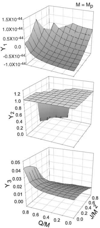
FIG. 13. Y1(fordM),Y2(fordJ), andY3(fordQ) as functions of J=M2 andQ=Mfor a solar mass black hole MM
s. It is
seen thatdJanddMhave negligible effect on2Stot, indicat-ing thatQfluctuations are the most significant here.
FIG. 12. Y1(fordM),Y2(fordJ), andY3(fordQ) as functions of J=M2 and Q=M for a Planck mass black hole MM
p.
Figure13shows the results for a solar mass black hole
MMs147 700 cm: (63)
Here,dJ is by far the least important, with dMmaking a larger, though still insignificant, contribution. dQ domi-nates and Q fluctuations, shown in Fig. 11, seem appro-priate. These are stable for all states.
V. CONCLUSIONS
I have worked out thermodynamic fluctuation theory for the Kerr-Newman black hole in an extensive, infinite en-vironment. Such an environment has the advantage that its character is irrelevant beyond the values of the three pa-rameters specifying its thermodynamic state. This is sig-nificant because the precise constitution of the universe is unknown (dark matter, etc). The known thermodynamics of the black hole is all that enters the structure of the theory. Although the full problem where allM; J; Qfluctuate is not stable, it seems reasonable to consider limited cases
where one or two of these conserved variables vary so slowly as to be considered fixed. These were all examined. All fluctuations with M fixed are stable everywhere in the physical regime. Scenarios withMfixed may be physi-cally the most relevant, as I argued with fluctuating parti-cles having roughly the properties of an electron. For a Planck mass black hole, J; Q fluctuations seem most significant. AsMincreases,Qfluctuations become domi-nant. Physically, perhaps most important are fluctuations in a nonrotating and uncharged environment, with average
JQ0. Here fluctuations are maximum and the sec-ond fluctuation moment forQis3:301e, independent ofM. The second fluctuation moment for J scales up linearly withM. For the Planck mass it is0:3990@. In cases where
M fluctuates, the transition from unstable (nearJQ 0) to stable is accompanied by infinite fluctuation moments.
[1] J. D. Bekenstein, Phys. Rev. D 7, 2333 (1973); 9, 3292 (1974).
[2] S. W. Hawking, Phys. Rev. D13, 191 (1976). [3] P. C. W. Davies, Proc. R. Soc. A353, 499 (1977). [4] L. D. Landau and E. M. Lifshitz, Statistical Physics
(Pergamon, New York, 1977).
[5] D. Tranah and P. T. Landsberg, Collective Phenomena 3, 81 (1980).
[6] L. Smarr, Phys. Rev. Lett.30, 71 (1973).
[7] C. W. Misner, K. S. Thorne, and J. A. Wheeler,Gravitation
(Freeman, San Francisco, 1973). [8] J. D. Bekenstein, Sci. Am., p. 58 (2003).
[9] B. Carter, inBlack Holes, edited by C. DeWitt and B. S. DeWitt (Gordon and Breach, New York, 1973).
[10] D. Pavo´n and J. M. Rubı´, Phys. Lett. A 99, 214 (1983); Gen. Relativ. Gravit.17, 387 (1985).
[11] J. Katz, I. Okamoto, and O. Kaburaki, Classical Quantum Gravity10, 1323 (1993).
[12] H. B. Callen, Thermodynamics and an Introduction to Thermostatistics(Wiley, New York, 1985).
[13] G. Arcioni and E. Lozano-Tellechea, Phys. Rev. D 72, 104021 (2005).
[14] J. E. A˚ man and N. Pidokrajt, Phys. Rev. D 73, 024017 (2006).
[15] M. E. Fisher, in Proceedings of the Gibbs Symposium, edited by D. G. Caldi and G. D. Mostow (American Mathematical Society and American Physical Society, Providence, Rhode Island, 1990).
[16] O. Kaburaki, Phys. Lett. A217, 315 (1996).
[17] S. Ferrara, G. W. Gibbons, and R. Kallosh, Nucl. Phys.
B500, 75 (1997).
[18] R. G. Cai and J. H. Cho, Phys. Rev. D 60, 067502 (1999).
[19] H. Eves, Elementary Matrix Theory (Dover, New York, 1966).
![Figure 1 shows M 2 p 3 . The values displayed are all nega- nega-tive. Indeed, Tranah and Landsberg [5] proved that p 3 < 0 for all states in the physical regime, violating the inequality Eq](https://thumb-us.123doks.com/thumbv2/123dok_us/8184705.2169761/4.918.476.843.63.334/figure-displayed-tranah-landsberg-proved-physical-violating-inequality.webp)