Antenna Response to CDM E-fields
Timothy J. Maloney
Intel Corporation, 2200 Mission College Blvd., SC9-09, Santa Clara, CA 95054 USA tel.: 408-765-9389 e-mail: [email protected]
This paper is co-copyrighted by Intel Corporation and the ESD Association
Abstract – The CDM event results from collapse of an electric dipole, producing an analytically describable radiation field pulse. A coaxial monopole E-field antenna’s transfer function gives the antenna signal in near-field, which features a bipolar “monocycle” pulse. A TLP-based synthetic monocycle pulser, for characterizing antenna-driven ESD detectors, is described.
I. Introduction
A Charged Device Model (CDM) ESD stress results when a charged component creates equal and opposite mirror charge in a ground plane, followed by collapse of the electric dipole in a current pulse when the affected pin touches ground. In recent years, workers have sought to measure such ESD events or monitor them in the factory by detecting radiated fields with a nearby antenna [1, 2]. This has achieved some static monitoring and control, but it has not been clear how to interpret the measured antenna waveforms in terms of the more familiar component CDM current waveforms and charge quantities. Also, factory tools are being outfitted with compact CDM ESD threshold detectors, fed by antennas situated near the possible source of ESD events. This motivates us to relate the yes/no thresholds of these electronic boxes, at a particular setting, to the expected properties of the antenna pulses coming in.
The author’s recent paper [3] described, in analytic form for free space, the small collapsing dipole pulses common to CDM events. These are pulsed Hertzian dipoles, much as long described in the literature for pulsed transmitting antennas but using a unique pole-zero treatment that captures all near and far fields (static field, induction field, radiated field) at once. This formulation, using complex frequencies to describe the current and field pulses, allows inversion to the time domain through the inverse Laplace Transform, and thus provides us with the basic building blocks of the CDM fields. Then we need to find the expected response of an antenna to that field. Our example will be a simple E-field antenna with a straightforward transfer function for the expected signal into a 50 ohm scope. As we will see, this pulse shape has been found to agree well with experiments, whereby an artificial CDM event produces a monitored current pulse and antenna signal simultaneously. The antenna is placed nearby (15 cm,
for example), as it would typically be in factory equipment. Given the propagation time to the antenna location (500 psec) and the expected speed of the event (nanosecond or sub-nanosecond pulses, rise times down to 100 psec or less), both the near fields and far field contribute, but this is all captured in one pole-zero expression as in [3], employable in both time and frequency domains.
Once the overall behavior of antenna signals for CDM is described, computed, and measured, we need to measure the effect of such signals on the compact ESD detector box, the yes/no threshold detector, at a particular setting. Does triggering primarily depend on peak-to-peak voltage, as expected? What is the influence of pulse speed, and is signal dispersion in the cable important? We will see how to replace the artificial air discharge CDM pulse and antenna with a highly reproducible synthetic pulse that has much more dynamic range and is easier to use. Starting with a familiar Transmission Line Pulse (TLP) system and using some expedient passive circuits, one can synthesize fast bipolar pulses resembling the E-field monopole antenna (made from coaxial cable and little else) response to CDM field pulses.
II. Pulsed Field Theory and Pulse
Generators
E, aligned with the current source and electric dipole
moment vector (z-direction), as this induces the largest signal in the antenna (Figure 1). In the s-domain,
c r s
s dl sr s I s
E
(1 ),
4 sin ) ( )
( 2 2
3 0
, (1)
where the polar angle =/2 at the equator, r is the distance from the source, c is the speed of light, dl is the length of the dipole. As explained in [3], the three terms describe the static field, induction field, and radiation field in the complex frequency domain. We will describe the current pulse I(s) once we see an example of a current pulse produced by dipole collapse.
The E-field of an electric dipole is the only field to which our E-field antenna is sensitive; the polar field E is the only E-field at the equator, as the radial field
Er vanishes there. Er depends only on static and inductive terms. Meanwhile, the associated magnetic field H is azimuthal and involves only the induction
and far-field radiation terms. These facts are well established in standard textbooks [4-6], but [3] offers a rare glimpse into the s-domain formulation (instead of setting s=j) and thus allows direct access to the pulsed field solutions that we need for CDM.
Figure 1. Experimental arrangement of CDM electric dipole initial source p and 6 mm coaxial antenna.
2. CDM-like Pulse Source and Model
A conceptual view of a generator of CDM-like pulses is shown in Figure 2. A charged plate with a spring loaded pogo pin comes down on a pedestal at the end of the center conductor of a 50-ohm coax line with its shield on the ground plane. The field created betweenthe charge plate and the ground plate then collapses and the current is detected by the 50-ohm scope connection. Note that any CDM spark resistance is in series with the 50 ohms, which raises the damping factor, simplifies the pulse, and makes ringing unlikely.
Figure 2. CDM pulse generator. Charge plate probe hits pedestal and dipole collapses, with current pulse and dipole radiation.
The top trace in Figure 3 shows the current pulse resulting from -100V applied to a pulse generator built as in Fig. 2, an instrument that has come to be known as the Charged Device Model Event Simulator (CDMES) [7]. A 3 GHz oscilloscope was used; the pulse has its peak and strongest derivatives in the first few hundred picoseconds.
We need a current function I(s) to approximate the pulse from this artificial CDM source. With a polynomial-based pole-zero expression, the fields can be computed using Heaviside inversion of the Laplace Transform [3]. The two-pole series RLC response to a step function is a favorite way to model a CDM pulse current [3] that occurs through capacitive discharge such as in Fig. 2. This is even the case with human body model (HBM) currents [8]. One can avoid field singularities by putting enough polynomial order in the denominator of E(s). We use high-speed poles to
model a step source with finite rise time for the spark, then multiply the familiar RLC expression for the rest of I(s) [3].
Figure 4a shows a calculated current pulse that approximates the experimentally measured CDMES current pulse as shown in Fig. 3, up to the trailing “ledge” on the measured pulse. Four poles were used
to
50
scope
p
15
cm
6
mm
“monopole”
antenna
on
50
cable
10
Meg
Charge
plate
Coax
to
50
ohm
scope
+V
Ground
plate
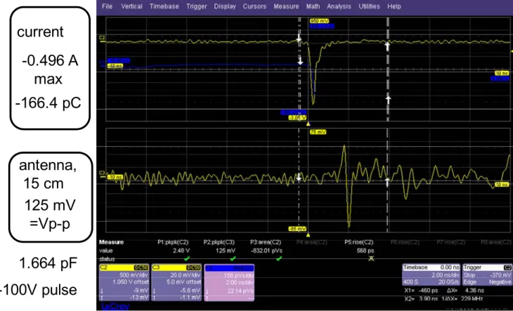
Figure 3. Measured current (top) and antenna response (bottom) to E-field at 15 cm, using artificial CDM source; 2 nsec/division, 3 GHz scope. Setup as in Fig. 1, current polarity negative. Integrated current gives -166.4 pC of charge; 10x attenuation used.
for the basic current pulse--two poles for the estimated 60 psec spark rise time and two more to capture the estimated RLC network (see Appendix), where R80 ohms (spark resistance + 50 ohms), L3 nH (probe inductance) and C1.66 pF (given by current integral from Fig. 3, although that includes the “ledge”). Then two more poles were added to capture the 3 GHz oscilloscope filtering, in accordance with models in [9]. With total charge reduced by 28% to adjust for the ledge, the current pulse then peaks at 0.49 amps, as calculated in Mathematica using Heaviside expansion to produce the inverse Laplace Transform.
The resulting E-field, in Figure 4b, is calculated from (1) for a 15 cm distance. The dipole moment length dl is about 4.5 mm, so the Hertzian dipole approximation is still good. Note that the resulting E-field is very sharp, showing the influence of the derivatives, particularly from the far-field (s2) term. Note also that while the CDM event is a collapsing dipole that starts out with nonzero static field and polarization (p in Fig. 1 is the initial dipole for a positive voltage), it is easiest to calculate the transient as a step in the polarization that ends at a finite value. This value, of course, cancels the initial static field.
Figure 4a. Calculated CDM current pulse, 1 nsec full scale.
Figure 4b. E-field pulse E at 15 cm from CDM current source as
in Fig. 4a; 1 nsec full scale.
-166.4 pC
antenna,
15 cm
current
1.664 pF
125 mV
=Vp-p
-100V pulse
-0.496 A
max
0.2 0.4 0.6 0.8 1.0
0.1 0.2 0.3 0.4 0.5
amps
nanosec
Volts/cm
0.2 0.4 0.6 0.8 1.0
-0.05 0.05 0.10 0.15 0.20 0.25 0.30
III.
Calculated and Measured
Antenna Pulses
The antenna used in these studies is a so-called monopole antenna made from coaxial cable. It is conceptually much as pictured in Fig. 1, aside from the Teflon cap over the 6 mm extension of the coaxial center conductor. A signal is generated as the E-field induces an electric dipole in the tip, driving the 50-ohm load. A simple circuit model gives the transfer function of such an antenna [10], and it can be applied as in [3] to give measured voltage Vm as
2 0
0 1
) (
) (
s C L s C Z
s C Z l s
E s V
m m m
m m
z m
, (2)
for which Z0 is cable impedance (usually 50 ohms), Cm and Lm are the inductive and capacitive equivalents of the probe wire, and lm is the length of the probe wire. The field E-z=E when maximum at
the equator, =/2, as before. The experimental setup, Fig. 1, defines positive polarity. To get the sign right, it is helpful to consider the initial induced dipole on the antenna; for a positive dipole as shown, there will be a net negative charge integrated from current during the collapse. The transfer function for our 6 mm probe is found from values suggested by [10], with Lm=5.1 nH and with a little more capacitance (Cm=0.38 pF) due to the Teflon cap. Combining (1) and (2), the “s” terms now cancel, so the signal will have no dc component, as expected, and will be influenced by the two new poles from the antenna. Sure enough, the predicted antenna signal as in Figure 5 shows a response to the sharp pulse of Fig. 4b that is influenced by ringing of the antenna itself. The dispersion along the coaxial cable (150 cm, RG-316) to the scope for such fast pulses was a concern, but calculations based on time-honored analysis [11] show that such effects should be negligible, only a picosecond or two for this cable length.
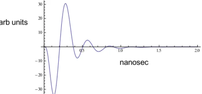
Figure 5. Calculated antenna response to E-field as in Fig. 4b, 15 cm from CDM source, 1.5 nsec full scale. Alignment as in Fig. 1.
Filtering by the 3 GHz scope bandwidth has been carried into the Fig. 5 calculations as well. The first two peaks of Fig. 5 match those of Fig. 3 almost
exactly, with -48.1 mV and +72.6 mV calculated in Fig. 5, versus +52 mV and -73 mV measured in Fig. 3 (Fig. 3 being flipped because of the -100V). But the third peak is not as prominent in Fig. 3 as in Fig. 5. Even so, only slight changes to the current function (so that it has a longer and smoother tail, a little closer to the “ledge” feature of Fig. 3) produces a predicted antenna pulse as in Figure 6, now having a reduced third peak although more balanced initial two peaks. As there is considerable estimation of the model parameters of the antenna and the discharge source, plus slight differences each time for air spark, plus effects of stray fields from the chargeup wire (which were reduced through careful design but are hard to eliminate completely), the agreement between theory and experiment is excellent. It’s a rare case of an ab initio pulsed field calculation followed by experiment. Such a crisp event as in Fig. 3 will not happen each time, but when it does, it’s a worst case, and its maximum current, field, and antenna signal can be associated with a maximum likelihood of device destruction if detected in the factory.
Figure 6. Calculated antenna response to E-field using a current source with a longer tail than Fig. 4a. 15 cm from CDM source, 2 nsec full scale, 3 GHz scope filter. Alignment as in Fig. 1.
The main feature of the antenna pulse is the prominent “monocycle” pulse up front, present in Figs. 3-6, with its overall peak-to-peak voltage Vp-p found in the swing of the first two peaks. We suspect that most CDM ESD detectors will be sensitive to Vp-p and now will show how to create easily reproducible monocycle pulses for detector characterization.
IV. Synthetic Antenna Pulses
1. Directional Couplers in the Time Domain
The expression for Vm, Eq. 2, converted to current given the 50 ohm scope input, indicates a small but finite current integral, given by the static charge on the antenna before collapse of the CDM dipole. This can just barely be discerned in Figs. 5-6 and looks like it may be lost in the noise in Fig 3. The antenna is much better as a sudden event detector and is not much of a static field meter! Accordingly, the 0.2 0.4 0.6 0.8 1.0 1.2 1.4-40
-20 20 40 60
nanosec millivolts
0.5 1.0 1.5 2.0
-30
-20
-10 10 20 30
arb units
monocycle pulse is nearly a balanced bipolar pulse for a typical CDM event. Thus we will allow our desired synthetic antenna pulse, something that easily characterizes an ESD detector, to have balanced pulse properties. We expect most ESD detectors to be kick-started by the peak-peak voltage Vp-p, and that the required time scale is short but not critical. Our target is to synthesize short bipolar pulses as a stand-in for less controllable “real” air discharge CDM pulses discussed above.
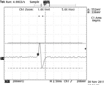
Earlier work [12] showed how a 3dB quarter wave directional coupler can be used to nearly differentiate a TLP step function, resulting in a CDM-like pulse at the sharp rising edge. There is only a single pulse if the TLP source has an RC termination as in [12], with a gradual decay of the falling edge. The monocycle pulse thus should result from the use of two successive quarter wave couplers, as in Figure 7. Figure 8 shows that indeed is the case. Note that Vp-p has a huge dynamic range over viable TLP voltages and attenuator choices, with the requirement of typical antenna Vp-p like 125 mV (Fig. 3) easily met. The scheme is quite suitable for synthesizing antenna-like pulses.
The monocycle pulse width is affected by scope speed, and the center frequencies of the directional couplers (0.75 and 1.5 GHz here).
Figure 7. TLP-based setup with two quarter-wave 3 dB couplers, aimed at producing a monocycle pulse.
Formally, the s-domain response of a coupler can be deduced from the standard frequency domain expression for the coupled signal [12-14]
sin cos
1
sin
2 1
2
j k
jk V
V
(3)
oo oe
oo oe
Z Z
Z Z k
, 20
, and ω0=2f0 is the ¼ wave angular frequency. Zoo and Zoe are the odd and even mode impedances, and all four ports are impedance matched, most often to 50 ohms. We can extend to all
complex frequencies by taking s=j,
k
'
1
k
2 ,Figure 8. Monocycle pulse output at 50V line charge, 10X attenuation, using scheme as in Fig. 7. Vp-p=552 mV after attenuation. 1 GHz scope, 2.5 nsec/division.
t0=1/4f0, the one-way transit time, and writing (3) as
1 coth ' sinh
cosh '
sinh )
( ) (
0 0
0 0 1
2
st k
k st
st k
st k s
V s V
. (4)
The response to a step V1(s)=V10/s and inversion to the time domain thus depend on finding an inverse Laplace Transform of (4), although the complete time series has been worked out [12,14].
The solution to (4) is, curiously, a scaled version of the basic TLP solution for an open-circuited line being switched into a resistive load. The circuit in Figure 9 is equivalent to such a case, and the input impedance of an open line of characteristic impedance Z0 is Z0 coth(st0), where t0 is the one-way transit time as above. Thus the loop admittance Y(s)=1/Z(s) is
d
R st Z
s Y
0 0coth
1 )
( . (5)
Figure 9. TLP circuit viewed in s-domain, equivalent to switching a Z0 line charged to -V0 into a load resistance Rd.
IN
90
0
ISO
IN
ISO
0 90
Step, from TLP
OUT, to 50 scope
90and ISO outputs are matched with 50
R
dZ
0,
t
0To get the current, multiply by voltage step V0/s, much as in (4), where V2(s) is a multiple of step voltage V1(s) whether V1(s) has finite rise time or not. Eqs. (4) and (5) are seen to be equivalent if k’/k is associated with Z0 and 1/k with Rd. Because coupling constant k<1, the TLP situation commensurate with the coupler would be for Rd>Z0. Now it is becoming clearer—the coupler wave series is the same as TLP into a resistor greater than the line impedance Z0, usually 50 ohms! That means no zero crossing in response to a pure step.
Following (5) and Fig. 9, by writing out the coth term in exponential form, it can be shown that
0 0 2 2 0 0
,
)
1
(
1
)
(
)
(
0 0Z
R
Z
R
e
e
R
Z
s
V
s
I
d d st st d
. (6)This is clearly a square pulse if =0, and always a series of steps of length 2t0. The solution in the time domain is
(7)
where u(t) is the unit step function. The same concepts can be applied to Eq. (4) to give
k
k
e
e
k
k
s
V
s
V
st st
1
1
,
)
1
(
1
)
1
(
)
(
)
(
0 0 2 2 1 2
(8)for the coupled line case. As (7) results from convolution with a step function, the time domain inversion of (4) and (8) must be
(9)
where (t) is the Dirac delta function. So indeed there is an inverse Laplace Transform for the likes of Eqs. (4) and (5), it’s just hard to find in mathematical tables. For example, (7) and (9) can be derived from item 29.3.66 in [15], but many steps are involved. The step response of a coupler was given by the author some time ago [12,14] but following a different treatment. Figure 10 is reproduced from [14] and represents (4) or (8) times 1V/s, or (9) convolved with a unit step function.
The coupler’s time domain impulse response, as on the right hand side of (9), is therefore the time derivative of the function in Fig. 10, a series of delta functions, first positive and then always negative. Note that the coupler operates best as a differentiator if k is small and the center frequency f0 is high
compared to, say, the reciprocal of the rise time of the step. For simulating antenna signals on the order of 100 mV using a TLP that easily produces pulses in the hundreds of volts, we can afford weak coupling. But Fig. 10 shows at a glance that even the fairly strong 3 dB coupler is not a bad differentiator if it is fast enough.
Figure 10. Ideal step response, on the coupled port, of a 3db (k=0.707) directional coupler, to an abrupt 1V traveling wave step on the input port. One time step is 2t0. From [14]; ©IEEE, 2005.
The monocycle pulser results from cascading two couplers, meaning that two functions like (8) plus a non-ideal step function are all multiplied, or two functions like (9) plus a suitable step function are all convolved. With proper choices we approximate the second derivative of the TLP step, as in Fig. 8. As noted earlier, the center frequencies of the two couplers used to produce Fig. 8 are 0.75 and 1.5 GHz, so t01=333 psec and t02=167 psec. These are commercial couplers, nominal 3 dB with estimated k=0.759 as discussed in [12].
2. Useful Approximations
It is useful to apply a polynomial approximation to (4), letting t0=t01 and noting series expansion
3 1 ) coth( 01 01 01 st st
st , so step response to
V1(s) = V10/s is
)
3
'
1
(
'
)
(
2 01 2 01 10 01 2
t
s
k
st
k
V
kt
s
V
, (10)after “s” terms cancel. The leading term of this (for s=0), when divided by Z0 to convert to current and charge, agrees with the Total Charge Theorem [12,14], although arriving at the result by different means. The Total Charge Theorem is now seen to be the leading term of an infinite series, the 0th moment
0 0.05 0.1 0.15 0.2 0.25 0.3 0.35 0.4 0.45
0 1 2 3 4 5
Tim e /Tim e of Flight
C oup le d V o lt ag e p er V o lt
nn d t n t u nt t u Z R V t
I
0 0 0 0
0 ( 2 ) ( (2 2) )
) (
nn t n t nt t k k s V s
V
0 0 0 12 ( 2 ) ( (2 2) )
or Q term of a current expression. This shows the power of the Laplace Transform analysis method. As shown, (10) is a two-pole approximation to the step response, and the series can be continued to approximate the step response with greater accuracy. Adding the second coupler with t02=1/4f02 convolves V2(s) with a related function times a factor of st02, i.e., nearly differentiates once again. The last contributor is the original TLP step V1(s) modified to have a finite rise time, and the monocycle pulse results. A generalized expression for the monocycle, with separate parameters for couplers 1 and 2, is
.
3
1
)
(
)
(
2 02 2 01 ' 2 ' 1
02 01 2 ' 2 02 ' 1 01 '
2 ' 1
2 02 01 2 1 1
t
t
k
k
t
t
s
k
t
k
t
s
k
k
s
t
t
k
k
s
V
s
V
m(11)
In a manner very similar to the CDM current, field and antenna signal calculations, these formulae were plugged into Mathematica to obtain plots as shown in Figure 11, a predicted monocycle pulse signal using the conditions as in the experiment of Fig. 8. In this calculation, the transit times t01 and t02 were as above, and k1=k2=0.759 as measured in [12]. Couplers were modeled as in (10), with each series cut off after the s2 term. Scope model was for 1 GHz in accordance with [9], D=0.707, and the pulse source V1(s) rise time, 10-90%, was 0.5 nsec, modeled as a pseudo-Gaussian (D=0.707), also in accordance with [9] and with [16].
Figure 11. Predicted monocycle signal for conditions of Fig. 8 using 2-pole approximations; 5 nsec full scale. Peak heights, ratios, pulse shape and time scale are all close to measured data.
Agreement of Fig. 11 with the Fig. 8 experiment is pretty good considering the numerous approximations and estimates. These simple methods should be adequate for choosing couplers for a desired experiment. It is well to remember that the coupler expressions, starting with the textbook Eq. (3), are customarily given in terms of the height of the incoming wave, V1, in a matched system, which will be half the charging voltage of the line for a TLP
pulse. However, in the TLP setup of Fig. 9 and Eq. (6), V0 is the full line charging voltage.
V. Calibration Example
The monocycle pulser is intended for easy calibration of an ESD event detector that is otherwise intended to pick up pulses from a monopole antenna. To simulate the antenna source more fully, the pulse should originate from a high impedance source, as the monopole antenna is a DC open circuit. This can be done by routing the pulse to the detector through a commercial pickoff tee [17] as shown in Figure 12. The 450 ohm output impedance will reflect nearly all of the signal reflected from the event detector, as would be the case with a monopole antenna. Signal strength is reduced by 10X, but there is still plenty of dynamic range to produce antenna-level signals (note that Fig. 8 required 10X attenuation at only 50V charge to avoid overloading the scope).
Figure 12. Using a 10X (20 dB) resistive pickoff tee in a 50-ohm system so that the monocycle pulser has high impedance, similar to the monopole antenna.
Next we tried out the monocycle pulse system on a compact ESD event detector with monopole antenna input that has recently become available, the MiniPulse® from Simco-Ion [18]. The pickoff tee of Fig. 12 and 150 cm of RG-316 cable was needed to simulate the monopole antenna and its 150 cm cable, because a substantial reflection from the event detector was found, as shown in Figure 13.
The MiniPulse event detector is set at an adjustable threshold sensitivity (1.2-1.9 volts) and initiates an alarm when an event is triggered. The setting relates to the output of internal logarithmic amplifiers, allowing a large dynamic range of antenna signals. Thus we hoped that our simple metric of “Vp-p of a fast monocycle pulse” would relate in a meaningful way to the setting of the MiniPulse event detector. Indeed that is the case for a 150 cm (5 ft) antenna cable with the monocycle pulse, shown in Figure 14.
1 2 3 4 5
-0.2
-0.1 0.1 0.2 0.3
Volts
nanosec
450 (20 dB)
Port 1 Port 2
Port 3
pulse in to 50 scope
Figure 13. Monocycle pulse (left, 175 mV=Vp-p) and its reflection from ESD event detector (right, 112 mV) after transit of 150 cm cable (15 nsec). Here the cable and event detector were on Port 2 and Port 3, 20 dB down, was routed to the oscilloscope.
Figure 14. Monocycle pulse peak-to-peak voltage (Vp-p) magnitude vs. threshold setting of MiniPulse event detector, semi-log plot. Excellent agreement with exponential fit (422 mV/decade).
The semi-log plot of Fig. 14 shows excellent agreement with an exponential fit, as anticipated from the use of the log amp. The MiniPulse does detect pulses weaker than 100 mV but we should clean up stray radiation from the TLP relay actuation to be confident of the data. Because of the reflection coefficients, the calibration data shown for the 150 cm cable in Fig. 14 does not apply to cables of different length, as the MiniPulse utilizes the resonant cavity formed by the cable. Trendlines for 300 and 450 cm cables (10 ft., 15 ft.) are above and to the left of the trendline in Fig. 14; thus the system is less sensitive to pulses for longer cables. The extreme case of an impedance-matched source turns out to be unacceptable for the MiniPulse event detector.
VI. Conclusions
The fields of a CDM-like pulse can be generated by using an air spark to collapse an electric dipole in a handheld instrument, one that also allows measurement of the current pulse. The E-fields nearby can be picked up and measured by a small “monopole” antenna, whose transfer function can be estimated from antenna dimensions. The result is a measured signal (combining static field, induction field, and radiation field) that is remarkably close to what is predicted from pulsed Hertzian dipole theory [3] from the known parameters, and affords considerable insight into the monitoring of actual CDM events in a semiconductor factory. Because the air spark is hard to control in the instrument and even harder to control in the factory (where we are trying to avoid it!), only the strongest events look just like the theoretical prediction, but those are the worst-case events of highest interest. The antenna waveforms can put definite bounds on the associated CDM event in terms of current and charge quantity, although complete “current imaging” from the antenna signal, as described in [3], remains a difficult goal.
It has been important to recognize the CDM radiation event as being well approximated by the pulsed Hertzian dipole, and as one that benefits from a pole-zero treatment in the s-domain. As described in [3], these tools have largely been overlooked in earlier reviews of pulsed Hertzian dipoles [19], where the tradition has been to use a Gaussian waveform, having no defined t=0, no oscillations, and freedom to choose only the time scale and strength of the pulse. In the present day, the inverse Laplace Transform is so readily available with math software, even as a free applet on the web [20], that the accepted method of acquiring a quick grasp of pulsed fields and signals really ought to change. The monopole antenna transfer function can be worked into the same pole-zero scheme through approximate models [3, 10] that are in reasonable agreement with more exact calculations [21]. This formulation of the field and signal expressions in the s-domain, with Heaviside inversion of the Laplace Transform into the time domain through computer tools, allows a complete and concise picture of the fields to be acquired quickly.
The main feature of a monopole antenna response to a CDM event is the fast bipolar pulse, with peak-peak voltage Vp-p of, usually, tens to hundreds of millivolts. Similar pulses (monocycle pulse) can be made very reproducibly by augmenting a TLP system with two high-speed directional couplers so that a
y = 0.1696e5.4535x
R² = 0.9927
100 1000 10000
1 1.2 1.4 1.6 1.8 2
Mo
n
o
cy
cl
e
Vp
‐
p,
mV
MiniPulse setting, V
non-ideal step is (nearly) differentiated twice. Time and frequency domain expressions for the monocycle pulse are presented, and approximations make it easy to design suitable pulse hardware. This artificial antenna pulse is useful for studying any kind of CDM ESD event detector, e.g., one aimed at replacing the oscilloscope in the factory with a small alarm box attached to the antenna. The CDM event detector studied here showed predictable response to antenna Vp-p over a wide dynamic range, owing to use of a logarithmic amplifier.
Appendix
While the polar field E(s) as in Eq. (1) is sufficient
for the experiments described herein, the remaining fields of the electric dipole in the s-domain are as follows [3]. The magnetic field is entirely azimuthal and has no static component:
sin
4
) 1 ( ) ( )
( 2
r s dl s I s
H . (A1)
Finally, the radial E-field Er(s) has a static component but vanishes in the far field:
s s r
dl s I s
Er
cos ) 1 ( 2
) ( )
( 3
0
. (A2)
Magnetic dipoles are totally analogous to electric dipoles, while exchanging the roles of E and H fields [3-6], but it is well to remember that the magnetic dipole is I(s) times an area, unlike I(s)/s (polarization) times dl for the electric dipole.
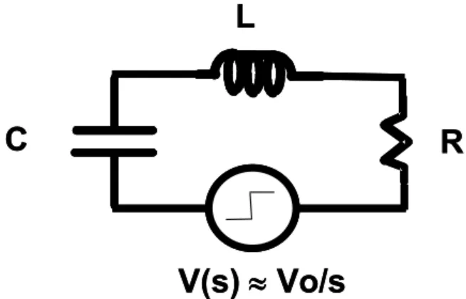
The I(s) expression used herein for the CDM-like pulse is also taken from [3] and starts with a 2-pole RLC model as in Figure A.1.
Figure A.1. Two-pole RLC model of CDM pulse.
The current function for Fig. A.1 is
1
)
(
2 0
RCs
LCs
CV
s
I
, (A3)and is readily integrated into the field expression, along with additional poles describing the finite rise time of the step source.
Acknowledgements
The author thanks Mark Hogsett, Lyle Nelsen and Steve Heymann of Simco-Ion (an ITW company) for lab work, and thanks Julian Montoya and Ghery Pettit of Intel for manuscript review. Also he thanks Joseph S. Hayden III of Intel for exploratory network analyzer studies of antennas and cables. Finally, the author wants to remember the late Tina Cantarero, who built all the major elements of the monocycle pulser at Intel, as described in [12].
References
[1] J.A. Montoya and T.J. Maloney, "Unifying Factory ESD Measurements and Component ESD Stress Testing", 2005 EOS/ESD Symposium, Sept. 2005, pp. 229-237. See https://sites.google.com/site/esdpubs/documents/e sd05.pdf.
[2] A. Jahanzeb, K. Wang, J. Harrop, J Brodsky, T. Ban, S. Ward, J. Schichi, K. Burgess and C. Duvvury, “Capturing Real World ESD Stress with Event Detector”, 2011 EOS/ESD Symposium, pp. 197-201.
[3] T.J. Maloney, "Easy Access to Pulsed Hertzian Dipole Fields Through Pole-Zero Treatment", cover article, IEEE EMC Society Newsletter, Summer 2011, pp. 34-42. See http://ewh.ieee.org/soc/emcs/acstrial/newsletters/s ummer11/index.html.
[4] S. Ramo, J. Whinnery, and T. Van Duzer, Fields and Waves in Communication Electronics (New York: John Wiley & Sons, 1965).
[5] J.B. Marion, Classical Electromagnetic Radiation (New York: Academic Press, 1965).
[6] J. D. Jackson, Classical Electrodynamics, 3rd Edition (New York: John Wiley and Sons, 1999). [7] Simco-Ion, Alameda, CA; private
communication.
[8] T.J. Maloney, "HBM Tester Waveforms, Equivalent Circuits, and Socket Capacitance", 2010 EOS/ESD Symposium, pp. 407-415. See https://sites.google.com/site/esdpubs/documents/e sd10.pdf.
[9] T.J. Maloney and A. Daniel, "Filter Models of CDM Measurement Channels and TLP Device Transients", 2011 EOS/ESD Symposium
C
V(s)
Vo/s
L
R
C
V(s)
Vo/s
L
Proceedings, pp. 386-394. See https://sites.google.com/site/esdpubs/documents/e
sd11.pdf.
[10] S. Caniggia and F. Maradei, "Numerical Prediction and Measurement of ESD Radiated Fields by Free-Space Field Sensors", IEEE Trans. on Electromagnetic Compatibility, vol. 49, no. 3, pp. 494-503 (Aug. 2007).
[11] R.L. Wigington and N.S. Nahman, "Transient Analysis of Coaxial Cables Considering Skin Effect", Proc. IRE, vol. 45, pp. 166-174, Feb. 1957.
[12] T.J. Maloney and S.S. Poon, "Using Coupled Transmission Lines to Generate Impedance-Matched Pulses Resembling Charged Device Model ESD", 2004 EOS/ESD Symposium, pp. 308-315. Also published in IEEE Trans. On Electronics Packaging Manufacturing, vol. 29, no. 3, pp. 172-178 (July 2006). See https://sites.google.com/site/esdpubs/documents/e sd04.pdf.
[13] G. Matthaei, L. Young, and E.M.T. Jones, Microwave Filters, Impedance-Matching Networks, and Coupling Structures (New York: McGraw-Hill, 1964; reprinted by Artech House, 1980), pp. 798-800.
[14] T.J. Maloney and S.S. Poon, "Total Charge Theorem for Directional Couplers and Z-matched Coupled Lines", IEEE Microwave and Wireless Components Letters, vol 15, pp. 413-415 (June 2005).
[15] M. Abramowitz and I.A. Stegun, Handbook of Mathematical Functions, (New York: Dover Publications, 1965).
[16] C. Mittermayer and A. Steininger, "On the Determination of Dynamic Errors for Rise Time Measurement with an Oscilloscope", IEEE Trans. on Instrumentation and Measurement, Vol. 48, no. 6, pp. 1103-07, Dec. 1999.
[17] Picosecond Pulse Labs, Inc.; web page at http://www.picosecond.com. Picosecond also offers a monocycle pulser.
[18] Simco-Ion (an ITW company), www.simco-ion.com.
[19] G. Franceschetti and C.H. Papas, “Pulsed Antennas”, IEEE Trans. on Antennas and Propagation, Vol. AP-22, No. 5, Sept. 1974, pp. 651-661. Also is a government report, online at http://www.ece.unm.edu/summa/notes/Sensor.htm l, SSN 203.
[20] Web resource,
http://www.eecircle.com/applets/007/ILaplace.ht ml.