https://www.phoenixpub.org/journals/index.php/jaar Journal of Applied and Advanced Research, 2019: 4(1) 1624 http://dx.doi.org/10.21839/jaar.2019.v4i1.263
ISSN 2519-9412 / © 2019 Phoenix Research Publishers
Research Article – Hydrology
Rainfall-runoff estimation of Bojiang lake watershed using SCS-CN model coupled with GIS
for watershed management
Nametso Matomela٭, Li Tianxin, Lehlohonolo Morahanye, Obadia Kyetuza Bishoge,
Harrison Odion Ikhumhen
School of Energy and Environmental Engineering, University of Science and Technology Beijing, Beijing 100083, PR China
(Received: 14-12-2018; Accepted 25-01-2019; Published Online 27-01-2019)
٭Corresponding author (E-mail: [email protected])
Abstract
A proper understanding of watershed spatio-temporal hydrological characteristics is critical to the management of a watershed and its natural resources such as water and vegetation. Rainfall runoff estimation plays an important role as an integral part of watershed management. Runoff volume and distribution data provides valuable information for water management strategies such as selection of artificial water abstraction sites, water storage facilities, and soil erosion control strategies. In the present study, Bojiang lake watershed was used to indicate the application of Soil Conservation Service Curve Number method (SCS-CN) coupled with Geographic Information System (GIS) and Remote Sensing (RS) techniques. The watershed falls within Erdos Larus Relictus National Nature Reserve (ELRNNR) which was listed under the wetlands of international importance in 2002. Rainfall runoff is influenced by a variety of factors within a watershed such as soil and land use/cover types, soil moisture content, rainfall, drainage density, and shape and size of the watershed. The SCS Curve number is the most popular and widely applied method for runoff estimation. GIS and Remote Sensing play an important role in estimating surface runoff by SCS-CN method. ArcGIS 10.2 software was used to overlay different thematic layers and develop an attribute table and calculate a weighted curve number. The weighted curve number was applied to the SCS-CN equations to estimate daily, monthly, and yearly runoff. Correlation coefficient (r) was used to test for the relationship between rainfall and runoff, and verify the computation of the method. The results show an average runoff of 17.78 mm which is about 7.18% of the annual average rainfall for the years 2001-2016. The derived output maps can assist in identifying suitable areas for water recharge/abstraction. The study demonstrates that SCS-CN in conjunction with GIS and RS can be used to calculate runoff for ungagged watersheds and assist in watershed management strategies.
Keywords: Rainfall-runoff; Remote Sensing; Soil Conservation Service; Watershed; GIS; Bojiang lake watershed.
Introduction
Water resources need to be carefully monitored and managed in order to achieve their sustainability and continue to be beneficial to the society. Watersheds are important units of which water and other natural resources can be strategically managed (Singh et al., 2017). A watershed is an area of land that drains water to a common outlet (Sindhu et al., 2013). Effects of climate change and gradually increasing human activities continue to put pressure on water as a scarce resource (Singh et al., 2017; Sample and Liu, 2014). Watersheds need to be carefully managed in order to use water resource wisely and optimally. Surface hydrological indications are one of the promising scientific tools for assessment and management of water resources (Ouyang et al., 2011; Viji et al., 2015). There is an urgent need for the evaluation of water resources as water plays a primary role in the sustainability of livelihoods and regional economy. A good understanding of hydrologic variability of a watershed or wetland is essential to develop effective management or restoration strategies (Ghobadi et al., 2012; Viji et al., 2015). Hydrological conditions of a wetland are one of the main factors affecting the status of wetland systems. Hydrologic modeling provides a means to help understand wetland hydrological processes under the influence of human activities and climate change (Ghobadi et al., 2012). Rainfall run off is one of the key hydrologic parameters to be considered in wetlands, watersheds, and water resource management (Viji et
al., 2015). Runoff estimation of a watershed facilitates the prediction of the probable amount of water drained by the watershed, development of water conservation strategies, and map out areas susceptible to soil erosion (Katara et al., 2013).
infiltration rate. SCS-CN has been widely applied as it is relatively easy to apply, simple, and reliable in getting results (Katara et al., 2013). Since the Bojiang catchment is relatively large, about 642km2, the SCS-CN method has been applied for the estimation of runoff. Tailor and Shrimali (2016), showed that runoff can be estimated using SCS-CN method together with GIS for proper watershed management. Dhawale (2013), applied SCS-CN method to approximate surface runoff depth when there is insufficient hydrologic information. The study demonstrated the significance of GIS and Remote Sensing data to obtain model parameters to estimate surface runoff from an ungauged watershed (Dhawale, 2013). The SCS-CN model was used together with remote and GIS to understand the correlation between runoff potential and Land use/Land cover, and correlation between runoff and soil condition (Dhawale, 2013). Kadam et al. (2012) applied the SCS-CN method to identify potential areas for construction of rainwater harvesting structures. Bhura et al. (2015) carried a study on surface runoff estimation from various land use types in Mapili watershed using SCS CN and GIS. The aforementioned method has been selected due to its wide application and capability to produce usable results that can be referred to in watershed management and natural resource conservation or restoration.
The Bojiang lake catchment is the only wetland in the world with the specific intent to protect the Larus Relictus (Relict Gull) and its habitats and was recorded in the List of Wetlands of International Importance in 2002 (Yan et al., 2017). The ungauged catchment has been seriously endangered by dryness and lake shrinkage, yet the hydrological processes in the catchment are poorly understood due to the lack of in-situ observations. Previous studies reported that water shortage in the catchment is mainly due to increased water consumption by human activities, and construction of silt trap dams (Yan et al., 2017) . Few studies have been done on the hydrology of the study area at
watershed or basin level especially taking into consideration the physiological characteristics of the watershed (Liang, 2017). The variations in stream flow were attributed to climate parameters (precipitation and evapotranspiration) and human activities (Liang, 2017). Precipitation and vegetation changes were the main factors contributing to Bojiang lake area variations (Yan et al., 2017). Estimation of runoff for Bojiang lake catchment is of great significance as the area is ungauged, therefore, prediction of runoff can assist in soil and water conservation plans for efficient watershed management. In the present study, SCS-CN model coupled with GIS and Remote Sensing has been used to estimate runoff for Bojiang lake catchment area.
Research methodology
Study area description
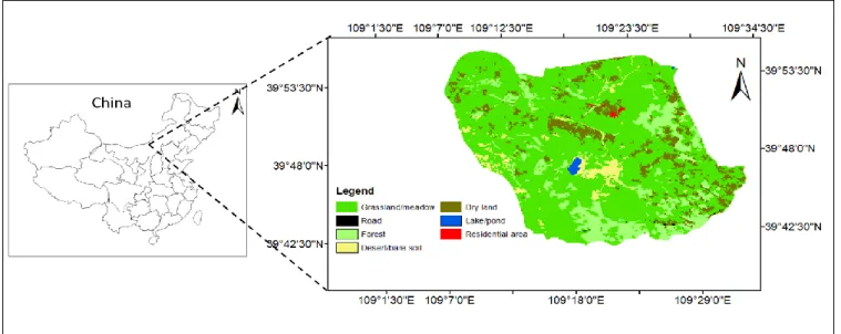
The Bojiang lake watershed is located within the in ELRNNR in Ordos City, Inner Mongolia Autonomous Region in China. The watershed is approximately 45 km to the west of Dongsheng District of Ordos City. The Bojiang lake basin lies between 109o7’0”E to 109o34’30”E longitude and 38o59’0”N to 39o42’30”N. The inland basin is situated in a semi-arid region and covers an area of about 642 km2. The yearly mean temperature of the basin is around 5.2oC. The yearly mean precipitation is approximately 247.53 mm, but the mean yearly evaporation capacity of the basin is about 2501 mm. Bojiang Lake is the largest lake in the basin, and two seasonal rivers named Jigou River and Porto River flow into the lake. Jigou and Porto river are the two seasonal rivers that flow into the Bojiang lake which is the biggest lake in the basin. The vegetation in the watershed mainly comprises of shrubs and grasses. The Bojiang Lake basin is a closed basin with an elevation of 1360-1600 m. The Lake is a shallow lake, with an average depth of 2.5 m and the deepest point of 9.0 m (Yan et al., 2017). Figure 1 below shows the location map of the study area.
Fig. 1. Location map of Bojiang lake watershed
Materials and methods
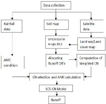
The methodology adopted in this study is outlined in Figure 2 which shows the different steps executed to finally estimate the watershed runoff. Daily rainfall data from 2001 to 2016 was obtained from Dongsheng meteorological station (Dongsheng National Reference station). A 30 x 30m DEM
https://www.phoenixpub.org/journals/index.php/jaar
Landsat 8 satellite image and topographic maps. Figure 3 shows the land use/land cover map. The soil types of the watershed were converted to hydrological soil groups B, C and D according to their infiltration properties. The land use map layer, and the derived hydrological soil group layer, were overlaid in Arcgis and used as inputs for the union tool (analysis tools) in order to derive polygon area of soil types (HSG) under each Land use/Land cover. A curve number, for each derived polygon, was determined based on the SCS-CN method standards and a weighted curve number (WCN) was calculated for AMC-I, II, and III. Finally, rainfall runoff was estimated using the equation provided by the SCS-CN method.
Fig. 2. Flow chart of methodology for runoff calculation by SCS-CN Model
SCS Curve Number Model
The SCS-CN was developed in the early 1950s by the United States Department of Agriculture (USDA) and the Natural Resource Conservation Society. This method can also be called the CN method and it was established to estimate rainfall runoff (Satheeshkumar et al., 2017; Rallison, 1980; Tailor and Shrimali, 2016). The SCS-CN is grounded on the water balance equation and the hypotheses which are outlined as follows, (a) ratio of the actual direct runoff to the potential runoff is equal to the ratio of the actual infiltration to the potential infiltration, and (b) the quantity of the initial abstraction is some fraction of the potential infiltration (Vandersypen et al., 1972). The USDA developed uncomplicated empirical equations and readily curves and tables which are applied in SCS method (Dhawale, 2013).
𝑄
(𝑃−𝐼𝑎)
=
𝐹
𝑆 …… (1)
𝐹 = (𝑃 − 𝐼𝑎) − 𝑄 ……(2)
Substituting Eq. (2) in eq. (1) and by solving;
𝑄 =
(𝑝−𝐼)2(𝑝−𝐼𝑎)+𝑠 ……(3)
Where, 𝑄 = actual runoff (mm), P=rainfall (mm), 𝐼𝑎=initial abstraction, which represents all the losses before
the runoff begins and is given by the empirical equation.
𝐼𝑎=0.2 𝑆 ……(4)
Substituting Eq. (4) in eq. (3); the eq. (3) becomes
𝑄 =(𝑝−0.2𝑠)(𝑝−0.8𝑠)2 For P>Ia (0.2S) ……(5)
𝑆 = the potential infiltration after the runoff begins given by following equation
𝑠 =25400
𝐶𝑁 − 254 ……(6)
CN is the curve number, a dimensionless number that range from 0-100, which is drawn from a table provided by the SCS handbook of Hydrology depending on the HSG, landuse/landcover , and AMC (Songara et al., 2015; Satheeshkumar et al., 2017; Amutha and Porchelvan, 2009). HSG is expressed in four groups which are A, B, C, and D, with A signifying the lowest rate of runoff potential and highest rate of infiltration, B and C moderate, and D signifies the highest runoff potential and lowest rate of infiltration. AMC is categorised into AMC I, II, and III depending on rainfall limits for dormant and growing seasons. The SCS CN method has been modified for larger watershed. Thus, for watersheds larger than 15 km2 the method can be applied by weighing curve numbers with regards to the land use/land cover areas of the watershed. The weighted curve number equation is shown below.
𝐶𝑁𝑤 =∑(𝐶𝑁𝑖∗𝐴𝑖)
𝐴 ……(7)
Where,
CNw= weighted curve number
CNi= curve number from to any number Ai= area with curve number CNi Antecedent moisture condition (AMC)
Antecedent moisture condition refers to the amount of water present in the soil at a given time (Mishra et al., 2004). AMC is an essential factor for deciding the final CN value. Three antecedent soil moisture conditions (AMC I, AMCII, AMCIII), were developed by the SCS according to conditions of the soil and precipitation limits for inactive and growing seasons. Table 2 shows the classification of Antecedent Moisture Condition. This study has taken AMC II which is average condition to determine the curve number value for Bojiang lake watershed.
Table 1. Group of Antecedent soil moisture classes (AMC)
AMC Group Soil Characteristics
Five-day antecedent rainfall (mm)
Dorman Growing season i Wet conditions. Soils are dry not
to wilting point, cultivation has taken place
<13 <36
ii Average conditions 13-28 36-53 iii Light or heavy rainfalls and low
temperatures have occurred within the last 5 days; saturated soils
>28 >53
AMC II (CNII) can be converted to the other AMC groups through the following correlation equation.
CNIII for AMC − I:2.281−(0.01281∗𝐶𝑁𝐼𝐼)𝐶𝑁𝐼𝐼 ……(9)
Hydrological soil group (HSG)
Topographic maps were scanned, georeferenced, and digitized in ArcGIS 10.2 software in order to produce all the necessary maps. The SCS model categorizes soil types into four groups which are A, B, C and D, in accordance with their infiltration rate (Sindhu et al., 2013). A HSG map was carefully produced based on the different types of soils in the watershed whereby each soil type was attributed to the hydrological soil group it belongs to. Classification of HSG is shown in table 2 in accordance with the SCS-CN standards. Hydrological soil group and Antecedent moisture content assists in determining the CN values. The method of
conservation was used to derive CN values for AMC I and II out of AMC II.
Land use/Land cover map
The land use/land cover map was produced with the help of data collected during the site visit of the study area. Remote sensing satellite images (Landsat) were also used as some areas were inaccessible during the field data collection. Thus, Remote Sensing data was complemented by the field data and subsequently both supervised and unsupervised classification were carried out using ARCGIS software. Finally, an output map was produced to show the classification of various land uses and land cover of the study area as shown in fig. 3.
Table 2. Hydrological soil Group Classification (Sindhu et al., 2013)
Fig. 3. (a) Land use cover map (b) Soil distribution map of Bojiang lake watershed Hydrological
soil Group
Description Minimum infiltration rate
(mm/hr) A Soils are characterized by high infiltration and low runoff potential even when
extremely wetted. These types of soil have high water transmission rate. They comprise of deep, well to exceedingly well drained sands or gravels.
7.62-11.43
B This group consists of soils with moderate infiltration rates when exceedingly wetted and consists primarily of moderately deep to deep, drained to moderately well-drained soils with moderately fine to moderately coarse textures. The water transmission rate of these soils is average.
3.81 – 7.62
C The soils have a slow infiltration rate when exceedingly wetted and comprises primarily of soils that have a layer which prevents percolation of water, or soils with fine to averagely fine texture. Thus, the rate of water transmission is slow for these soils.
1.27- 3.81
D Soils have very slow infiltration rate and therefore the runoff potential is high when thoroughly wetted. They comprise primarily of clay soils with high everlasting high-water table, high swelling potential, soils with a layer of clay close to the surface, and shallow soils on top of material which is not easily allowing passage of water.
0-1.27
https://www.phoenixpub.org/journals/index.php/jaar
Table 3. Calculation of weighted curve number for Bojiang Lake watershed
SR No. Land use cover Soil type
(HSG)=) CN (Km
2) %AREA %AREA*CN WEIGHTED CN
1 dry land B 72 9 1.4019608 100.9411744 58.26891905 =AMC I
C 81 21 3.2712418 264.9705829 76.13025227=AMC II D 86 32 4.9847494 428.6884444 88.19268859=AMC III 2 residential area B 72 0.138189 0.0215262 1.549884439
C 81 2 0.3115468 25.2352936
D 86 3 0.4673203 40.18954167
3 forest B 66 4 0.6230937 41.12418217
C 77 15 2.3366013 179.918297
D 83 79 12.3061 1021.406297
4 Desert/bare soil B 72 8 1.2461873 89.72548837
C 81 3 0.4673203 37.85294041
D 86 17.247387 2.6866844 231.0548595
5 Lake/pond _ 100 2 0.3115468 31.15468346
6 grassland/meadow B 58 52.572479 8.1893947 474.9848932
C 71 134 20.873638 1482.028292
D 78 259 40.345315 3146.934577
7 Road D 98 1 0.1557734 15.2657949
Weighted area curve number
Cumulative Departure from the mean (CDM)
The cumulative departure from the mean is a method which is widely applied when analyzing time series data such as precipitation and temperature data (Yan et al., 2017). The method is used to show trends through accumulated departure curves. The CDM was calculated using the following formula:
CMD = ∑𝑛𝑖=1(𝑥𝑖− 𝑥̅)/𝑥̅ ……(10)
where CMD is the cumulative departure from the mean, 𝑥𝑖 is a single value in a time series data, and 𝑥̅ is the mean
value of the time series data.
The CMD method was used to analyze rainfall data for the period 2001-2017.
Pearson correlation coefficient
The Pearson correlation coefficient, also called Pearson’s r is an extensively used method used to measure correlation between two variables (Yan et al., 2017). The correlation coefficient (r) is a dimensionless numeric value that ranges from -1 to 1. Thus, the coefficient value determines the significance of the correlation. A correlation coefficient of 0 indicates that there is no linear relation between two variables. If the coefficient is 1 or very close to 1, it shows that the two variables have a positive linear correlation. The correlation coefficient is calculated using the following formula;
Fig. 4. (a) Curve number map (b) Hydrological soil group map
𝑟 = ∑𝑛𝑖=1(𝑥𝑖−𝑥̅)(𝑦𝑖−𝑦̅) √∑𝑛𝑖=1(𝑥𝑖−𝑥̅)2∑𝑛𝑖=1(𝑦𝑖−𝑦̅)2
……(11)
Where r is the correlation coefficient, 𝑥𝑖 and 𝑦𝑖 are the
single values of the two variables. 𝑥̅ and 𝑦̅ are the mean values of the time series data for the two variables. The Pearson correlation coefficient was used to calculate the correlation between rainfall and runoff in the watershed.
Results and discussion
Curve numbers and Hydrological soil group maps
The weighted curve numbers were computed for dry, wet, and normal conditions as showed in Table 3. Equation 3 was used to calculate weighted curve number for AMC II (normal condition). Curve numbers for wet (AMC I) and dry condition (AMC III) were derived from weighted CN for normal conditions using Equations 9 and 8. The calculated curve numbers were 58.27, 76.13, and 88.19 for AMC I, II, and III respectively.
A CN grid map was created using the Geospatial Hydrologic Modelling Extension (HEC-GeoHMS), a geospatial hydrology extension that is used within ArcGIS to develop hydrologic modelling inputs. The data sets added to the HEC-GeoHMS include DEM, soil-land use polygon and a curve number lookup table.
A soil distribution map of the watershed was developed using GIS as indicated in Figure 4. The soil types were mapped out using fieldwork and auxiliary data. The soil types outlined include fluro-aquic soil, chestnut soil, regosol soil, light chestnut colored soil, grey desert soil, meadow soil, and prairie wind-blown soil. The soil distribution map assisted in the development of the HSG map based on the various soil types and their properties such as infiltration rate and potential for runoff. The derived HSG map is shown in Figure 5 which indicated that a significant area of the watershed, about 60.79%, is covered by soils that belong to HSG D. Therefore, most of the area is covered by soils which have low infiltration rate and high runoff potential when thoroughly wetted.
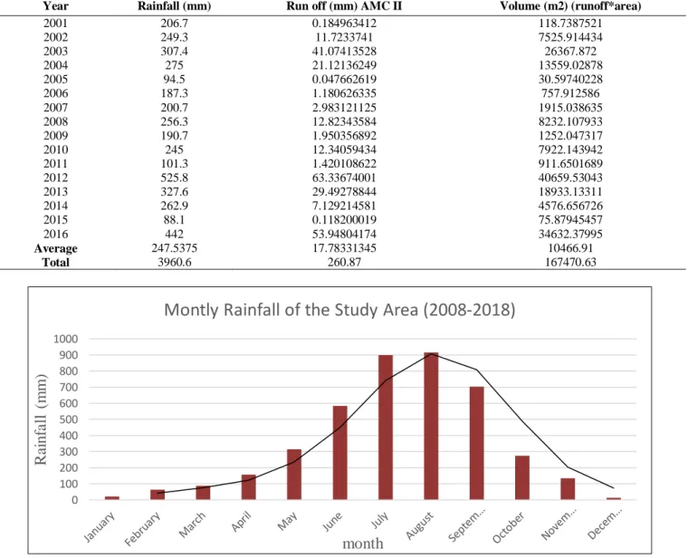
Table 4. Rainfall-runoff depth and volume (2001-2016)
Year Rainfall (mm) Run off (mm) AMC II Volume (m2) (runoff*area)
2001 206.7 0.184963412 118.7387521
2002 249.3 11.7233741 7525.914434
2003 307.4 41.07413528 26367.872
2004 275 21.12136249 13559.02878
2005 94.5 0.047662619 30.59740228
2006 187.3 1.180626335 757.912586
2007 200.7 2.983121125 1915.038635
2008 256.3 12.82343584 8232.107933
2009 190.7 1.950356892 1252.047317
2010 245 12.34059434 7922.143942
2011 101.3 1.420108622 911.6501689
2012 525.8 63.33674001 40659.53043
2013 327.6 29.49278844 18933.13311
2014 262.9 7.129214581 4576.656726
2015 88.1 0.118200019 75.87945457
2016 442 53.94804174 34632.37995
Average 247.5375 17.78331345 10466.91
Total 3960.6 260.87 167470.63
Fig. 5. monthly rainfall and moving average of the study area
Rainfall and runoff in the catchment area
The rainfall data from 2001-2016 was collected from Dongsheng meteorological station. The rainfall runoff of Bojiang lake watershed ranges from 0.04 mm to 63.3 mm
(2001-2016) as shown in table 4. Maximum runoff was observed in 2012 which was about 24.28% of the total rainfall and the minimum was observed in 2005 about 0.02%. The rainfall ranges between 88.1mm and 525.8mm as shown in Table 4, and most of the rainfall occurred in the months of
0 100 200 300 400 500 600 700 800 900 1000
R
ai
n
fa
ll
(
m
m
)
month
https://www.phoenixpub.org/journals/index.php/jaar
July, August, and September, as indicated in Figure 5. Average annual rainfall runoff is 17.78 mm which equates to 7.18% of the average annual rainfall, whereas the average runoff volume for the 16-year period is 167470.63 m2. The variation of rainfall and runoff depth is presented in Figure 5. The apparent low rainfall-runoff proportion might be due to the reason that the study area is semi-arid with low intensity rainfall and infrequent rainfall events over time. Rainfall runoff is also influenced by land use and land cover types, slope and soil type distribution across the watershed. The study area consists of different land cover types, however it is
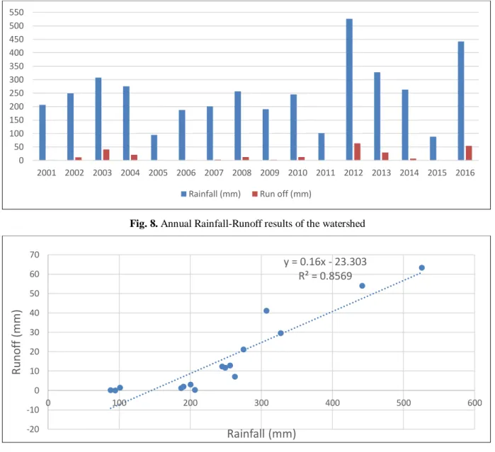
dominated by grassland/meadow (69.41%) and forest (15.27%) land covers. A scatter plot was created to measure the linear relationship between rainfall and runoff. The rainfall and runoff were correlated and the correlation coefficient (r2) was found to be 0.86, thus showing a positive strong relationship between rainfall and runoff in the study area. Surface runoff verification could not be carried out since the study is an ungagged catchment. Nonetheless, considering the reliability and the wide application of the SCS-CN model for runoff estimation, the obtained results are regarded as satisfactory (Senay and Verdin, 2004; Mahmoud, 2014).
Fig. 6. Rainfall variation for Bojiang lake watershed
Fig. 7. Annual precipitation trend and cumulative departure from the mean (2001-2016)
The trend of precipitation changes and cumulative departure from the mean were calculated as shown in Figure 6. Figure 6 generally shows a strong fluctuation in the trend of annual precipitation from 2001-2016. As shown in Figure 7 precipitation was generally below average from 2004 until 2011. The annual precipitation increased drastically and reached its peak in 2012.
Conclusion
The study demonstrates that the use of SCS-CN method couple with GIS is a viable way to estimate rainfall runoff in an ungagged watershed. The method can significantly assist in the effective management of a watershed and water resources. Accurate prediction of rainfall runoff using conventional methods can be laborious and time consuming.
However, remote sensing together with GIS can greatly support the estimation of runoff. The method presented is cost effective and yields relatively accurate results. The total annual surface runoff of 17.78mm represents about 7.18% of the total annual rainfall in the watershed. Antecedent moisture condition and CN values are of great significance and need to be carefully determined when calculating runoff. The rate of runoff depth depends on the Curve number values which are decided based on the soil and land use cover types. The results obtained also show that runoff potential differs with land use/cover and soil characteristics. In the present study, the CN values for AMC I to AMC III have been found to be 58.26, 76.13, 88.19, respectively. The relationship between rainfall and runoff was tested using correlation coefficient (r2) and the result showed a positive
206.7 249.3
307.4 275
94.5
187.3200.7 256.3
190.7 245
101.3 525.8
327.6 262.9
88.1 442
330.7
0 100 200 300 400 500 600
R
AI
N
FALL
(M
M
)
YEARS Rainfall (mm)
-2 -1.5 -1 -0.5 0 0.5 1 1.5
2000 2002 2004 2006 2008 2010 2012 2014 2016 2018
pr
ec
ip
it
at
io
n
depa
rt
ur
e
fr
o
m
t
he
m
ean
year
Fig. 8. Annual Rainfall-Runoff results of the watershed
Fig. 9. Rainfall-Runoff relationship
relationship between the two variables. The SCS-CN method proves to be efficient, cost effective, and can be applied to large areas to map out sites for artificial water recharge or abstraction. Therefore, the method can be applied as an integral part of land and water resources in order to achieve sustainable development.
References
Amutha, R., and Porchelvan, P. (2009). Estimation of surface runoff in Malattar sub-watershed using SCS-CN method. Journal of the Indian Society of Remote Sensing, 37(2), 291–304.
Bhura, C.S., Singh, N.P., Mori, P.R., Prakash, I. and Mehmood, K. (2015). Estimation of Surface Runoff For Ahmedabad Urban Area using SCS-CN Method and GIS. International Journal of Science Technology & Engineering, 1(11), 411–416.
Dhawale, A.W. (2013). Runoff Estimation for Darewadi Watershed using RS and GIS. International Journal of Recent Technology and Engineering, 1(6), 46–50. Senay, G.B., and Verdin, J.P. (2004). Developing index
maps of water-harvest potential in Africa. Applied Engineering in Agriculture, 20(6), 789–799.
Ghobadi, Y., Pradhan, B., Kabiri, K., Pirasteh, S., Shafri,
H.Z.M., and Sayyad, G.A. (2012). Use of multi-temporal remote sensing data and GIS for wetland change monitoring and degradation. In IEEE Colloquim on Humanities, Science & Engineering Research. pp. 103–108.
Kadam, A.K., Kale, S.S., Pande, N.N., Pawar, N.J., and Sankhua, R.N. (2012). Identifying Potential Rainwater Harvesting Sites of a Semi-arid, Basaltic Region of Western India, Using SCS-CN Method. Water Resources Management, 26(9), 2537–2554.
Katara, P., Machiwal, D., Mittal, H.K., Dashora, Y., and Bhagat, A.D. (2013). Estimation of Runoff for Ahar River Catchment in Udaipur District Integrated Remote Sensing and Geographical Information System. The Institute of Engineers (India), Udaipur Local Centre, (July 2016), 169–175. Retrieved from internal-pdf://194.46.46.255/Katara-2013-Estimation of Runoff for Ahar Rive.pdf
Liang, K. (2017). Quantifying streamflow variations in ungauged lake basins by integrating remote sensing and water balance modelling: A case study of the erdos Larus relictus National Nature Reserve, China. Remote Sensing, 9. 588.
Mahmoud, S.H. (2014). Investigation of rainfall-runoff modeling for Egypt by using remote sensing and GIS
0 50 100 150 200 250 300 350 400 450 500 550
2001 2002 2003 2004 2005 2006 2007 2008 2009 2010 2011 2012 2013 2014 2015 2016
Rainfall (mm) Run off (mm)
y = 0.16x - 23.303 R² = 0.8569
-20 -10 0 10 20 30 40 50 60 70
0 100 200 300 400 500 600
Ru
n
o
ff
(mm)
https://www.phoenixpub.org/journals/index.php/jaar integration. Catena, 120, 111–121.
Mishra, S.K., Jain, M.K., and Singh, V.P. (2004). Evaluation of the SCS-CN-based model incorporating antecedent moisture. Water Resources Management, 18(6), 567– 589.
Ouyang, N.L., Lu, S.L., Wu, B.F., Zhu, J.J., and Wang, H. (2011). Wetland restoration suitability evaluation at the watershed scale- A sase study in upstream of the Yongdinghe River. Procedia Environmental Science, 10, 1926–1932.
Rallison, R.E. (1980). Origin and evolution of the SCS runoff equation. ASCE, 912–924.
Sample, D.J., and Liu, J. (2014). Optimizing rainwater harvesting systems for the dual purposes of water supply and runoff capture. Journal of Cleaner Production, 75, 174–194.
Satheeshkumar, S., Venkateswaran, S., and Kannan, R. (2017). Rainfall–runoff estimation using SCS–CN and GIS approach in the Pappiredipatti watershed of the Vaniyar sub basin, South India. Modeling Earth Systems and Environment, 3(1), 24.
Sindhu, D., Shivakumar, B.L., and Ravikumar, A.S. (2013). Estimation of Surface Runoff in Nallur Amanikere Watershed Using Scs-Cn Method, 404–409.
Singh, L.K., Jha, M.K., and Chowdary, V.M. (2017).
Multi-criteria analysis and GIS modeling for identifying prospective water harvesting and artificial recharge sites for sustainable water supply. Journal of Cleaner Production, 142, 1436–1456.
Songara, J. C., Joshipura, H. T. K. N. M., & Prakash, I. (2015). Estimation of Surface Runoff of Machhu Dam III Chatchment Area , Morbi , Gujarat , India , using Curve Number Method and GIS, 3(03), 2038–2043.
Tailor, D., and Shrimali, N.J. (2016). Surface runoff estimation by SCS curve number method using gis for Rupen-Khan watershed , Mehsana district , Gujarat soil. Journal of Indian Water Resources Society, 36(4), 2–6.
Vandersypen, D.R., Bali, J.S., and Yadav, Y.P. (1972). Handbook of hydrology. Government of India-Ministry of Agriculture, Central Unit for Soil Conservation, New Delhi.
Viji, R., Prasanna, P.R., and Ilangovan, R. (2015). Modified SCS-CN and Green-Ampt Methods in Surface Runoff Modelling for the Kundahpallam Watershed, Nilgiris, Western Ghats, India. Aquatic Procedia, 4, 677–684.