An IPv6 Deployment Guide
TABLE OF CONTENTS...V
LIST OF FIGURES... XI
LIST OF TABLES...XIII
LIST OF TABLES...XIII
FOREWORD ... XIV
PART I IPV6 FUNDAMENTALS... 1
CHAPTER 1 INTRODUCTION ... 3
1.1 THE HISTORY OF IPV6 ... 3
1.2 THE 6NETPROJECT... 5
CHAPTER 2 IPV6 BASICS ... 7
2.1 DATAGRAM HEADER... 7
2.2 HEADER CHAINING... 9
2.3 ROUTING HEADER... 11
2.4 FRAGMENTATION... 12
2.5 OPTIONS... 13
CHAPTER 3 ADDRESSING ... 15
3.1 ADDRESSING ESSENTIALS... 15
3.2 UNICAST ADDRESSES... 16
3.3 INTERFACE IDENTIFIER –MODIFIED EUI-64 ... 17
3.4 ANYCAST ADDRESSES... 18
3.5 MULTICAST ADDRESSES... 19
3.6 REQUIRED ADDRESSES AND ADDRESS SELECTION... 19
3.7 REAL-WORLD ADDRESSES... 21
CHAPTER 4 ESSENTIAL FUNCTIONS AND SERVICES... 24
4.1 NEIGHBOUR DISCOVERY... 24
4.1.1 Router Discovery... 25
4.1.2 Automatic Address Configuration ... 25
4.1.3 Duplicate Address Detection ... 26
4.1.4 Neighbour Unreachability Detection ... 27
4.1.5 Router Configurations for Neighbour Discovery ... 27
4.2 THE DOMAIN NAME SYSTEM... 42
4.2.1 Overview of the DNS ... 42
4.2.2 DNS Service for 6NET ... 43
4.2.3 DNS Service Implementation ... 44
4.3 DHCPV6 ... 52
4.3.1 Using DHCP Together With Stateless Autoconfiguration ... 52
4.3.2 Using DHCP Instead of Stateless Autoconfiguration ... 52
4.3.3 Overview of the Standardisation of DHCPv6 ... 52
4.3.4 Overview of the DHCPv6 Specifications... 54
4.3.5 DHCPv6 Implementations Overview... 55
CHAPTER 5 INTEGRATION AND TRANSITION... 59
5.1 PROBLEM STATEMENT... 59
5.1.1 Dual Stack ... 60
5.1.2 Additional IPv6 Infrastructure (Tunnels) ... 61
5.1.3 IPv6-only Networks (Translation) ... 61
5.2 TUNNELLING METHODS... 62
5.2.1 Configured Tunnels... 62
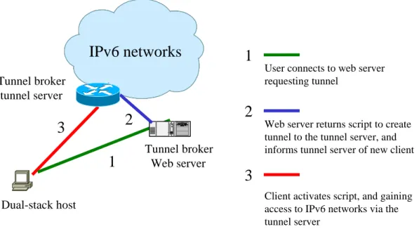
5.2.2 Tunnel Broker... 62
5.2.3 Automatic Tunnels... 64
5.2.7 Teredo... 66
5.2.8 Tunnel Setup Protocol... 67
5.2.9 Dual Stack Transition Mechanism (DSTM) ... 67
5.2.10 The Open VPN based Tunnelling Solution ... 70
5.3 TRANSLATION METHODS... 74
5.3.1 SIIT, NAT-PT and NAPT-PT... 74
5.3.2 Bump in the Stack... 74
5.3.3 Bump in the API ... 76
5.3.4 Transport Relay... 77
5.3.5 SOCKS... 79
5.3.6 Application Layer Gateway ... 79
5.3.7 The ‘Trick or Treat’ DNS-ALG... 80
5.4 CONFIGURATION EXAMPLES:DUAL STACK... 82
5.4.1 Dual-stack VLANs ... 82
5.5 CONFIGURATION EXAMPLES:TUNNELLING METHODS... 86
5.5.1 Manually Configured Tunnels ... 86
5.5.2 6over4 ... 94
5.5.3 6to4 ... 94
5.5.4 ISATAP ... 100
5.5.5 OpenVPN Tunnel Broker ... 106
5.5.6 DSTM... 116
5.6 CONFIGURATION EXAMPLES:TRANSLATION METHODS... 125
5.6.1 NAT-PT... 125
5.6.2 ALG... 127
5.6.3 TRT ... 134
CHAPTER 6 ROUTING ... 140
6.1 OVERVIEW OF IPROUTING... 140
6.1.1 Hop-by-hop Forwarding ... 140
6.1.2 Routing Tables... 141
6.1.3 Policy Routing ... 142
6.1.4 Internet Routing Architecture ... 143
6.1.5 Is IPv6 Routing Any Different?... 145
6.2 IMPLEMENTING STATIC ROUTING FOR IPV6... 146
6.2.1 Cisco IOS... 146
6.2.2 Juniper JunOS ... 148
6.2.3 Quagga/Zebra ... 149
6.3 RIP ... 151
6.3.1 RIPng Protocol... 151
6.4 IMPLEMENTING RIPNG FOR IPV6... 153
6.4.1 Cisco IOS... 154
6.4.2 Juniper JunOS ... 161
6.4.3 Quagga ... 165
6.5 IMPLEMENTING IS-IS FOR IPV6 ... 167
6.5.1 Cisco IOS... 167
6.5.2 Juniper JunOS ... 177
6.6 IMPLEMENTING OSPF FOR IPV6 ... 181
6.6.1 LSA Types for IPv6... 181
6.6.2 NBMA in OSPF for IPv6... 182
6.6.3 Cisco IOS... 183
6.6.4 Juniper JunOS ... 186
6.6.5 Quagga ... 189
6.7 IMPLEMENTING MULTIPROTOCOL BGP FOR IPV6... 192
6.7.1 Cisco IOS... 192
6.7.2 Juniper JunOS ... 201
6.7.3 Quagga/Zebra ... 201
7.1.2 MIBs ... 205
7.1.3 The Other Standards ... 206
7.1.4 Flow Monitoring (IPFIX, Netflow...)... 206
7.1.5 Management of IPv6 Protocols and Transition Mechanisms ... 207
7.1.6 Remaining Work to be Done ... 207
7.2 NETWORK MANAGEMENT ARCHITECTURE... 207
7.2.1 Conceptual Phase... 207
7.2.2 Implementation Phase - Management Tools Set ... 209
7.3 MANAGEMENT TOOLS DEPLOYED IN 6NET ... 210
7.3.1 Management Tools for Core Networks (WAN) ... 211
7.3.2 Management Tools for End-sites (LAN) ... 214
7.3.3 Tools for all Networks... 217
7.4 RECOMMENDATIONS FOR NETWORK ADMINISTRATORS... 218
7.4.1 Network Management Architecture ... 218
7.4.2 End-site Networks ... 218
7.4.3 Core Networks... 218
CHAPTER 8 MULTICAST ... 220
8.1 ADDRESSING AND SCOPING... 220
8.1.1 Well Known / Static Addresses ... 222
8.1.2 Transient Addresses ... 222
8.1.3 Summary ... 224
8.2 MULTICAST ON THE LOCAL LINK... 224
8.2.1 Multicast Listener Discovery (MLD)... 224
8.2.2 MLD Snooping ... 225
8.3 BUILDING THE MULTICAST TREE:PIM-SMV2... 225
8.4 INTER-DOMAIN MULTICAST... 226
8.4.1 The ASM Case ... 226
8.4.2 The SSM Case... 229
8.4.3 Future Work ... 230
8.5 MRIB-MULTICAST ROUTING INFORMATION BASE... 230
8.5.1 Extensions to BGP (MBGP)... 231
CHAPTER 9 SECURITY... 232
9.1 WHAT HAS BEEN CHANGED IN IPV6REGARDING SECURITY? ... 232
9.1.1 IPSec... 232
9.1.2 IPv6 Network Information Gathering... 233
9.1.3 Unauthorised Access in IPv6 networks ... 234
9.1.4 Spoofing in IPv6 Networks... 235
9.1.5 Subverting Host Initialisation in IPv6 Networks... 235
9.1.6 Broadcast Amplification in IPv6 Networks ... 236
9.1.7 Attacks Against the IPv6 routing Infrastructure ... 237
9.1.8 Capturing Data in Transit in IPv6 Environments ... 237
9.1.9 Application Layer Attacks in IPv6 Environments ... 237
9.1.10 Man-in-the-middle Attacks in IPv6 Environments ... 237
9.1.11 Denial of Service Attacks in IPv6 Environments... 238
9.2 IPV6FIREWALLS... 239
9.2.1 Location of the Firewalls ... 239
9.2.2 ICMP Filtering ... 242
9.3 SECURING AUTOCONFIGURATION... 245
9.3.1 Using Stateless Address Autoconfiguration ... 245
9.3.2 Using Privacy Extensions for Stateless Address Autoconfiguration ... 245
9.3.3 Using DHCPv6... 245
9.3.4 Static Address Assignment ... 246
9.3.5 Prevention techniques ... 246
9.3.6 Fake router advertisements... 246
9.4 IPV4-IPV6CO-EXISTENCE SPECIFIC ISSUES... 248
9.4.4 ISATAP ... 253
9.4.5 Teredo... 253
9.4.6 GRE Tunnels... 255
9.4.7 OpenVPN Tunnels ... 255
9.4.8 Dual-stack ... 256
9.4.9 DSTM... 257
9.4.10 NAT-PT/NAPT-PT... 258
9.4.11 Bump in the API (BIA) ... 259
CHAPTER 10 MOBILITY ... 260
10.1 BINDINGS CACHE... 260
10.2 HOME AGENT OPERATION... 261
10.3 CORRESPONDENT NODE OPERATION... 262
10.4 BINDING CACHE COHERENCE... 263
10.4.1 Binding Update Messages... 263
10.4.2 Binding Acknowledgement Messages ... 264
10.4.3 Binding Request Messages... 264
10.4.4 Binding Update List ... 264
10.5 PROXY NEIGHBOUR DISCOVERY... 264
10.6 HOME ADDRESS OPTION... 265
10.7 HOME AGENT DISCOVERY... 265
10.8 THE MOBILITY HEADER... 266
10.9 THE RETURN ROUTABILITY METHOD... 267
10.10 AVAILABLE IMPLEMENTATIONS... 268
10.11 DEPLOYMENT CONSIDERATIONS... 269
10.11.1 Hardware Requirements ... 269
10.11.2 Software Requirements ... 270
10.12 CISCO MOBILE IPV6 ... 271
10.12.1 Available Feature Set... 271
10.12.2 How to Get it ... 271
10.12.3 Installation ... 271
10.12.4 Configuration ... 272
10.12.5 Configuration Commands... 272
10.12.6 Operation... 275
10.13 MOBILE IPV6 FOR LINUX... 276
10.13.1 How to get it ... 276
10.13.2 Installation ... 276
10.13.3 Configuration ... 277
10.13.4 Usage Notes/Problems... 280
10.14 KAMEMOBILE IPV6... 281
10.14.1 How to get it ... 281
10.14.2 Installation ... 281
10.14.3 Configuration ... 282
10.14.4 Remarks ... 284
CHAPTER 11 APPLICATIONS ... 286
11.1 THE NEW BSDSOCKETS API... 287
11.1.1 Principles of the New API Design ... 287
11.1.2 Data Structures ... 288
11.1.3 Functions ... 290
11.1.4 IPv4 Interoperability... 296
11.2 OTHER PROGRAMMING LANGUAGES... 296
11.2.1 Python... 296
11.2.2 Java... 298
PART II CASE STUDIES ... 301
CHAPTER 12 IPV6 IN THE BACKBONE ... 303
12.1.3 Naming Scheme ... 309
12.1.4 DNS... 311
12.1.5 IGP Routing... 311
12.1.6 EGP Routing... 314
12.2 SURFNET CASE STUDY (NETHERLANDS) ... 316
12.2.1 The SURFnet5 Dual Stack network ... 316
12.2.2 Customer Connections ... 317
12.2.3 Addressing plan... 317
12.2.4 Routing ... 319
12.2.5 Network Management and Monitoring... 319
12.2.6 Other Services ... 320
12.3 FUNETCASE STUDY (FINLAND) ... 322
12.3.1 History ... 322
12.3.2 Addressing Plan ... 324
12.3.3 Routing ... 325
12.3.4 Configuration Details... 326
12.3.5 Monitoring... 329
12.3.6 Other Services ... 329
12.3.7 Lessons Learned... 330
12.4 RENATERCASE STUDY (FRANCE) ... 331
12.4.1 Native Support... 331
12.4.2 Addressing and Naming ... 331
12.4.3 Connecting to Renater 3 ... 332
12.4.4 The Regional Networks ... 333
12.4.5 International Connections... 333
12.4.6 Tunnel Broker Service Deployment ... 334
12.4.7 Network Management ... 335
12.4.8 IPv6 Multicast ... 336
12.5 SEERENCASE STUDY (GRNET) ... 337
12.5.1 SEEREN Network... 337
12.5.2 Implementation Details of CsC/6PE Deployment ... 339
CHAPTER 13 IPV6 IN THE CAMPUS/ENTERPRISE ... 341
13.1 CAMPUS IPV6DEPLOYMENT (UNIVERSITY OF MÜNSTER,GERMANY)... 341
13.1.1 IPv4... 342
13.1.2 IPv6... 343
13.1.3 IPv6 Pilot... 344
13.1.4 Summary ... 352
13.2 SMALL ACADEMIC DEPARTMENT,IPV6-ONLY (TROMSØ,NORWAY) ... 354
13.2.1 Transitioning Unmanaged Networks ... 354
13.2.2 Implementation of a Pilot Network... 355
13.2.3 Evaluation of the Pilot Network... 360
13.2.4 Conclusions ... 362
13.3 LARGE ACADEMIC DEPARTMENT (UNIVERSITY OF SOUTHAMPTON)... 364
13.3.1 Systems Components ... 364
13.3.2 Transition Status ... 370
13.3.3 Supporting Remote Users... 372
13.3.4 Next Steps for the Transition... 372
13.3.5 IPv6 Transition Missing Components ... 373
13.4 UNIVERSITY DEPLOYMENT ANALYSIS (LANCASTER UNIVERSITY) ... 374
13.4.1 IPv6 Deployment Analysis ... 374
13.4.2 IPv6 Deployment Status ... 378
13.4.3 Next Steps ... 380
13.5 OTHER SCENARIOS... 384
13.5.1 Early IPv6 Testbed on a Campus ... 384
13.5.2 School Deployment of IPv6 to Complement IPv4+NAT ... 385
13.5.3 IPv6 Access for Home Users... 385
CHAPTER 14 IPV6 ON THE MOVE ... 387
14.1 FRAUNHOFER FOKUS... 387
14.1.1 MIPL-HA ... 388
14.1.2 Kame-HA ... 388
14.1.3 MCU-CN ... 389
14.1.4 IPSec... 389
14.2 TESTBED COMPONENTS... 389
14.3 LANCASTER UNIVERSITY... 391
14.3.1 The Testbed... 391
14.3.2 Components ... 392
14.3.3 Addressing and Subnetting ... 393
14.3.4 Testing ... 394
14.4 UNIVERSITY OF OULU... 400
14.4.1 Testbed... 400
14.4.2 Handover Performance... 400
BIBLIOGRAPHY... 403
GLOSSARY OF TERMS AND ACRONYMS ... 412
APPENDICES... 419
APPENDIX A1: LIST OF PER-POP LOCATION SUPPORT DOMAINS ... 419
APPENDIX A2: SYSTEMS PROVIDING DNS SERVICE FOR 6NET... 420
Figure 2-1 Basic IPv6 Datagram Header ... 7
Figure 2-2 IPv4 and IPv6 Header Comparison... 9
Figure 2-3 Header Chaining Examples... 11
Figure 2-4 Changes in the Routing Header During Datagram Transport ... 12
Figure 3-1 Structure of the Global Unicast Address ... 16
Figure 3-2 Real-world Structure of the Global Unicast Address ... 17
Figure 3-3 Conversion of MAC Address to Interface Identifier ... 18
Figure 3-4 Structure of the IPv6 Multicast Address ... 19
Figure 3-5 Structure of the Real-world Global Unicast Address Prefix ... 22
Figure 5-1 Tunnel broker components and setup procedure ... 63
Figure 5-2 6to4 Service Overview ... 64
Figure 5-3 Teredo Infrastructure and Components... 66
Figure 5-4 DSTM Architecture ... 68
Figure 5-5 Tunnel Broker Scenario... 70
Figure 5-6 Interaction of tunnel broker components ... 71
Figure 5-7 Types of Tunnel Broker Clients... 72
Figure 5-8 The BIS Protocol Stack ... 75
Figure 5-9 The BIA Protocol Stack ... 76
Figure 5-10 Transport Relay Translator in Action ... 78
Figure 5-11 ALG Scenario ... 80
Figure 5-12 Sample Address Assignment and Routing Configuration... 111
Figure 5-13 Sample Subnet Routing ... 111
Figure 5-14 Test Network Infrastructure ... 116
Figure 5-15 Example Setup of Faithd TRT ... 137
Figure 6-1 Classical IP Forwarding ... 141
Figure 6-2 Internet Routing Architecture... 144
Figure 6-3 RIPng Message ... 152
Figure 7-1 The Unified MIB II ... 206
Figure 8-1 The MSDP Model... 227
Figure 8-2 Embedded-RP Model ... 228
Figure 8-3 MRIB and RIB... 231
Figure 9-1 Internet-router-firewall-protected Network Setup ... 240
Figure 9-2 Internet-firewall-router-protected Network Setup ... 241
Figure 9-3 Internet-edge-protected Network Setup ... 241
Figure 10-1 MIPv6 Routing to Mobile Nodes (Pre Route Optimisation)... 262
Figure 10-2 Mobile IPv6 Routing to Mobile Nodes (Post Route Optimisation) ... 262
Figure 10-3 The Mobility Header Format... 266
Figure 10-4 Return Routability Messaging... 267
Figure 10-5 Simple Mobile IPv6 Testbed... 269
Figure 11-1 Partial Screenshot of the Applications Database ... 286
Figure 12-1 The 6NET Core and NREN PoPs ... 304
Figure 12-2 6NET IS-IS Topology ... 312
Figure 12-3 BGP peering with 6NET participants ... 314
Figure 12-4 Logical topology for SURFnet5... 317
Figure 12-5 Anonymous-FTP over IPv6 volume ... 320
Figure 12-6 Funet Network by Geography ... 323
Figure 12-7 Funet Network by Topology ... 324
Figure 12-8 The Renater3 PoP Addressing Scheme... 331
Figure 12-9 Density of IPv6 Connected Sites on Renater3... 332
Figure 12-10 The Renater3 Network ... 334
Figure 12-11 The RENATER Tunnel Broker... 335
Figure 12-12 IPv6 Traffic Weathermap... 336
Figure 12-13 SEEREN Physical Network Topology ... 337
Figure 12-14 SEEREN Logical Topology ... 338
Figure 12-15 Label Exchange in the CsC Model ... 338
Figure 12-16 Routing Exchange in SEEREN... 339
Figure 13-1 Ideal Overview of University’s IPv4 Network ... 342
Figure 13-5 Traffic Statistics of Røstbakken Tower and faithd ... 360
Figure 13-6 Use of IPv6 VLANs at Southampton... 370
Figure 13-7 MRTG Monitoring Surge Radio Node (top) and RIPE TTM view (bottom)... 372
Figure 13-8 Basic Configuration of the Upgrade Path ... 378
Figure 13-9 Alternative Configuration Providing Native IPv6 to the Computing Dept ... 380
Figure 14-1 Schematic Representation of the Testbed Setup... 388
Figure 14-2 Lancaster University MIPv6 Testbed ... 391
Figure 14-3 Simple MIPv6 Handover Testbed... 396
Figure 14-4 Processing Router Solicitations... 397
Figure 14-5 University of Oulu Heterogeneous Wireless MIPv6 Testbed ... 400
Figure 14-6 TCP Packet Trace During Handover from AP-5 to AP-4 ... 401
Table 2-1 Extension Headers ... 10
Table 2-2 Hop-by-hop Options ... 13
Table 2-3 Destination Options ... 14
Table 3-1 IPv6 Address Allocation... 21
Table 3-2 Global Unicast Address Prefixes in Use ... 21
Table 5-1 The Teredo Address Structure... 66
Table 8-1 IPv6 Multicast Address Format... 220
Table 8-2 The Flags Field ... 220
Table 8-3 Multicast Address Scope ... 221
Table 8-4 Permanent IPv6 Multicast Address Structure ... 222
Table 8-5 Unicast Prefix-based IPv6 Multicast Address Structure... 223
Table 8-6 Embedded RP IPv6 Multicast Address Structure ... 223
Table 8-7 SSM IPv6 Multicast Address Structure... 223
Table 8-8 Summary of IPv6 Multicast Ranges Already Defined (RFCs or I-D) ... 224
Table 9-1 Bogon Filtering Firewall Rules in IPv6 ... 234
Table 9-2 Structure of the Smurf Attack Packets ... 236
Table 9-3 ICMPv6 Recommendations... 244
Table 10-1 Mobile IPv6 Bindings Cache... 261
Table 10-2 IPv6 in IPv6 Encapsulation ... 261
Table 10-3 IPv6 Routing Header Encapsulation ... 263
Table 10-4 Mobile IPv6 Home Address Option ... 265
Table 10-5 Available MIPv6 Implementations ... 268
Table 10-6 MIPL Configuration Parameters ... 278
Table 11-1 Values for the Hints Argument... 293
Table 12-1 6NET Prefix ... 305
Table 12-2 PoP Addressing... 306
Table 12-3 SLA Usage ... 306
Table 12-4 Switzerland Prefixes ... 307
Table 12-5 Loopback Addresses ... 307
Table 12-6 6NET PoP to NREN PoP Point-toPoint-Links ... 308
Table 12-7 Point-to-point links between 6NET PoPs... 309
Table 12-8 Link Speed IS-IS Metric... 313
Table 12-9 CLNS Addresses... 314
Table 12-10 SURFnet Prefix... 318
Table 12-11 SURFnet prefixes per POP ... 318
Table 14-1 Fokus MIPv6 Testbed Components ... 389
Table 14-2 Lancaster MIPv6 Testbed Components ... 392
Table 14-3 Results of RA Interval Tests... 397
Table 14-4 Using Unicast RAs... 398
Viviane Reding, European Commissioner for Information Society and Media
Large scale roll-out trials of Internet Protocol version 6 (IPv6) are a pre-requisite for competitiveness and economic growth, across Europe and beyond. Progress in research, education, manufacturing and services, and hence our jobs, prosperity and living standards all ultimately depend on upgrades that improve the power, performance, reliability and accessibility of the Internet. Europe is fast becoming the location of choice for the world’s best researchers. Why? Because Internet upgrade projects like 6NET have helped to give Europe the world’s best climate for collaborative research. Thanks to 6NET, we have high-speed, IPv6-enabled networks linking up all of our research centres and universities, and supporting collaboration on scales that were impossible only a few years ago. Europe’s GÉANT network, which supplies vast number crunching power to researchers across Europe and beyond, is completely IPv6-enabled and is already carrying vast amounts of IPv6 traffic. Pioneering work by the 6NET consortium has made IPv6 know-how available to help school networks to upgrade IPv6 wherever IPv4 can no longer cope.
PART I
IPv6
Chapter 1
Introduction
Internet Protocol version 6 (IPv6) is the new generation of the basic protocol of the Internet. IP is the common language of the Internet, every device connected to the Internet must support it. The current version of IP (IP version 4) has several shortcomings which complicate, and in some cases present a barrier to, the further development of the Internet. The coming IPv6 revolution should remove these barriers and provide a feature-rich environment for the future of global networking.
1.1
The History of IPv6
The IPv6 story began in the early nineties when it was discovered that the address space available in IPv4 was vanishing quite rapidly. Contemporary studies indicated that it may be depleted within the next ten years – around 2005! These findings challenged the Internet community to start looking for a solution. Two possible approaches were at hand:
1. Minimal: Keep the protocol intact, just increase the address length. This was the easier way promising less pain in the deployment phase.
2. Maximal: Develop an entirely new version of the protocol. Taking this approach would enable incorporating new features and enhancements in IP.
Because there was no urgent need for a quick solution, the development of a new protocol was chosen. Its original name IP Next Generation (IPng) was soon replaced by IP version 6 which is now the definitive name. The main architects of this new protocol were Steven Deering and Robert Hinden. The first set of RFCs specifying the IPv6 were released at the end of 1995, namely, RFC 1883: Internet Protocol, Version 6 (IPv6) Specification [RFC1883] and its relatives. Once the definition was available, implementations were eagerly awaited. But they did not come.
The second half of the nineties was a period of significant Internet boom. Companies on the market had to solve a tricky business problem: while an investment in IPv6 can bring some benefits in the future, an investment in the blossoming IPv4 Internet earns money now. For a vast majority of them it was essentially a no-brainer: they decided to prefer the rapid and easy return of investments and developed IPv4-based products.
Another factor complicating IPv6 deployment was the change of rules in the IPv4 domain. Methods to conserve the address space were developed and put into operation. The most important of these was Classless Inter-Domain Routing (CIDR). The old address classes were removed and address assignment rules hardened. As a consequence, newly connected sites obtained significantly less addresses than in previous years.
eyes of those who were relatively new to the Internet. Since the Internet was booming, requests for new address blocks were increasing, yet the size of assigned address blocks were being reduced. Thus, new or expanding sites had to develop methods to spare this scarce resource. One of these approaches is network address translation (NAT) which allows a network to use an arbitrary number of non-public addresses, which are translated to public ones when the packets leave the site (and vice versa). Thus, NATs provided a mechanism for hosts to share public addresses. Furthermore, mechanisms such as PPP and DHCP provide a means for hosts to lease addresses for some period of time.
The widespread deployment of NAT solutions weakened the main IPv6 driving force. While IPv6 still has additional features to IPv4 (like security and mobility support), these were not strong enough to attract a significant amount of companies to develop IPv6 implementations and applications. Consequently, the deployment of IPv6 essentially stalled during this period.
Fortunately, the development of the protocol continued. Several experimental implementations were created and some practical experience gained through to operation of the 6bone network. This led to the revisited set of specifications published in the end of 1998 (RFC 2460 and others).
An important player in the IPv6 field has always been the academic networks, being generally keen on new technologies and not that much interested in immediate profit. Many of them deployed the new protocol and provided it to their users for experimentation. This brought a lot of experience and also manpower for further development.
Probably the most important period for IPv6 so far has been the first years of the 21st century, when IPv6 finally gained some momentum. The increasing number of implementations forced remaining hardware/software vendors to react and to enhance their products with IPv6 capabilities.
The new protocol also appeared in a number of real-world production networks. Network providers in Asia seemed to be especially interested in IPv6 deployment. The reason for this is clear – the Internet revolution started later in these countries, so they obtained less IPv4 addresses and the lack of address space is thus considerably more painful here. In short, the rapid growth of Internet connectivity in Asia cannot be served by the relatively miniscule IPv4 address space assigned to the region. This even led to some governments declaring their official support for IPv6.
The deployment of IPv6 in Europe has been boosted by the Framework Programmes of European Commission. Funding was granted for projects like 6NET and Euro6IX that focused on gaining practical experience with the protocol. Also, the largest European networking project - the academic backbone GÉANT – would include IPv6 support once sufficient confidence and experience had been gained from the 6NET project.
The main focus of the GÉANT project was to interconnect national research and education networks in European countries. As these networks were interested in IPv6, its support in the backbone was one of the natural consequences. After a period of experiments, IPv6 has been officially provided by GÉANT since January 2004.
Euro6IX focused on building a pan-European non-commercial IPv6 exchange network. It interconnected seven regional neutral exchange points and provided support for some transition mechanisms. Other objectives were to research and test IPv6-based applications over the infrastructure and disseminate the experience.
Between 2000 and 2004, the vast majority of operating system and router vendors implemented IPv6. These days it is hard to find a platform without at least some IPv6 support. Although the implementations are not perfect yet (advanced features like security or mobility are missing in many of them), they provide a solid ground for basic usage. Moreover, in most cases one can see dramatic improvements from one release to the next.
1.2 The
6NET
Project
6NET was a three-year European IST project to demonstrate that continued growth of the Internet can be met using new IPv6 technology. The project built and operated a pan-European native IPv6 network connecting sixteen countries in order to gain experience of IPv6 deployment and the migration from existing IPv4-based networks. The network was used to extensively test a variety of new IPv6 services and applications, as well as interoperability with legacy applications. This allowed practical operational experience to be gained, and provided the possibility to test migration strategies, which are important considering that IPv4 and IPv6 technologies will need to coexist for several years. 6NET involved thirty-five partners from the commercial, research and academic sectors and represented a total investment of €18 million; €7 million of which came from the project partners themselves, and €11 million from the Information Society Technologies Programme of the European Commission. The project commenced on 1st January 2002 and was due to finish on 31 December 2004. However, the success of the project meant that it was granted a further 6 months, primarily for dissemination of the project’s findings and recommendations. The network itself was decommissioned in January 2005, handing over the reigns of pan-European native IPv6 connectivity to GÉANT. The principal objectives of the project were:
• Install and operate an international pilot IPv6 network with both static and mobile components in order to gain a better understanding of IPv6 deployment issues.
• Test the migration strategies for integrating IPv6 networks with existing IPv4 infrastructure.
• Introduce and test new IPv6 services and applications, as well as legacy services and applications on IPv6 infrastructure.
• Evaluate address allocation, routing and DNS operation for IPv6 networks.
• Collaborate with other IPv6 activities and standardisation bodies.
• Promote IPv6 technology.
The project had important collaborations with other IPv6 activities such as the Euro6IX project and the IPv6 Cluster, and contributed to standardisation bodies such as the IETF (Internet Engineering Task Force) and GGF (Global Grid Forum). 6NET also played an important role in promoting IPv6 technology at both the national and international level.
6NET has demonstrated that IPv6 is deployable in a production environment. Not only does it solve the shortage of addresses, but it also promises a number of enhanced features which are not an integral part of IPv4. The success of the testbed spurred the existing GÉANT and NORDUnet networks to move to dual-stack operation earlier than anticipated, and in turn, encouraged many NRENs (National Research and Education Networks) to offer production IPv6 services as well. Having served its purpose, and with 6NET partners now having native IPv6 access via GÉANT, the 6NET testbed was decommissioned in January 2004. During its lifetime, the 6NET network was used to provide IPv6 connectivity to a number of worldwide events, including IST 2002 (November 2002), IETF 57 (July 2003), IST 2003 (November 2003) and the Global IPv6 Service Launch (January 2004), showing that it is ready for full deployment.
The experience gained during the project has been turned into a number of ‘cookbooks’ (project deliverables) aimed at network administrators, IT managers, network researchers and anyone else interested in deploying IPv6. All project documentation: deliverables, papers, presentations, newsletters etc., are freely available on the 6NET website:
http://www.6net.org/
providing all the important information in a single reference book is much more preferable to the reader than negotiating our multitude of project deliverables.
We hope you find this reference book informative and that it helps smooth your IPv6 deployment process. Please bear in mind that this book is a ‘snapshot in time’ and by the very nature of IPv6 protocols and their implementations it is easy for the information in these chapter to become out of date. Nevertheless, through the 6DISS project many ex-6NET partners will endeavour to keep the information up to date and you can freely download the latest electronic version from the 6NET website:
http://www.6net.org/book/
The 6NET project was co-ordinated by Cisco Systems and comprised:
ACOnet (Austria) Telematica Instituut (Netherlands) CESNET (Czech Republic) TERENA
DANTE UKERNA (UK)
DFN (Germany) ULB (Belgium)
ETRI (South Korea) UCL (UK)
FCCN (Portugal) University of Southampton (UK)
GRNET (Greece) CSC (Finland)
HUNGARNET (Hungary) CTI (Greece)
IBM DTU (Denmark)
GARR (Italy) Fraunhofer FOKUS (Germany) Lancaster University (UK) INRIA (France)
NORDUnet Invenia (Norway)
NTT (Japan) Oulu Polytechnic (Finland)
PSNC (Poland) ULP (France)
Chapter 2
IPv6 Basics
Inside this chapter we cover the protocol basics: the datagram format, the headers and related mechanisms. You will see that these aspects have been simplified significantly in comparison to IPv4 to achieve higher performance of datagram forwarding.
2.1 Datagram
Header
The core of the protocol is naturally the datagram format defined in RFC 2460 [RFC2460]. The datagram design focused mainly on simplicity - to keep the datagram as simple as possible and to keep the size of the headers fixed. The main reason for this decision was to maximise processing performance - simple constant size headers can be processed quickly, at or very close to wire-speed. The IPv4 header format contains a lot of fields including some unpredictable optional ones leading to fluctuating header sizes. IPv6 shows a different approach: the basic header is minimised and a constant size. Only essential fields (like addresses or datagram length) are contained. Everything else has been shifted aside into so called extension headers, which are attached on demand - for example a mobile node adds mobility related extension headers to its outgoing traffic.
Figure 2-1 Basic IPv6 Datagram Header
Version
Protocol version identification. It contains value 6 to identify IPv6.
Traffic Class
Intended for the Quality of Service (QoS). It may distinguish various classes or priorities of traffic (in combination with other header fields, e.g. source/destination addresses).
Flow Label
Identifies a flow which is a “group of related datagrams”.
Payload Length
Length of the datagram payload, i.e. all the contents following the basic header (including extension headers). It is in Bytes, so the maximum possible payload size is 64 KB.
Next Header
The protocol header which follows. It identifies the type of following data - it may be some extension header or upper layer protocol (TCP, UDP) data.
Hop Limit
Datagram lifetime restriction. The sending node assigns some value to this field defining the reach of given datagram. Every forwarding node decreases the value by 1. If decremented to zero, the datagram is dropped and an ICMP message is sent to the sender. It protects the IPv6 transport system against routing loops - in the case of such loop the datagram circulates around the loop for a limited time only.
Source Address
Sender identification. It contains the IPv6 address of the node who sent this datagram. Addressing is described in more detail in the next chapter.
Destination Address
Receiver identification. This is the target - the datagram should be delivered to this IPv6 address.
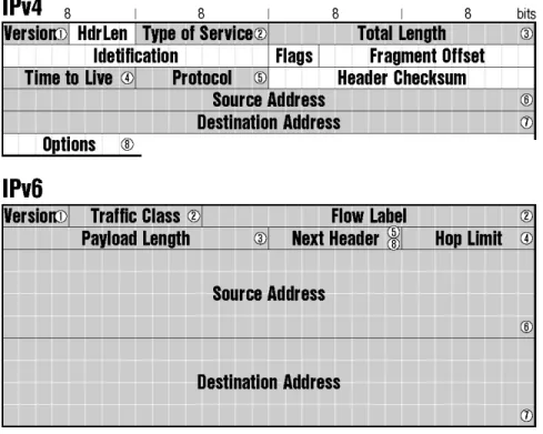
Before we dive deeper into some header specialties let us compare the IPv4 and IPv6 headers (see Figure 2-2). The result is quite interesting: the total length of the datagram header doubled (from 20 bytes to 40 bytes) although the IPv6 addresses are four times as long.
Figure 2-2 IPv4 and IPv6 Header Comparison
2.2 Header
Chaining
Instead of placing optional fields to the end of datagram header IPv6 designers chose a different approach - extension headers. They are added only if needed, i.e. if it is necessary to fragment the datagram the fragmentation header is put into it.
Extension headers are appended after the basic datagram header. Their number may vary, so some flexible mechanism to identify them is necessary. This mechanism is called header chaining. It is implemented using the Next Header field. The meaning of this field in short is to identify “what follows”.
Actually, the Next Header field has two duties: it determines the following extension header or identifies the upper-layer protocol to which the datagram content should be passed. Because many datagrams are plain - they do not need any extension header at all. In this case the Next Header simulates the Protocol field form IPv4 and contains value identifying the protocol (e.g., TCP or UDP) which ordered the data transport.
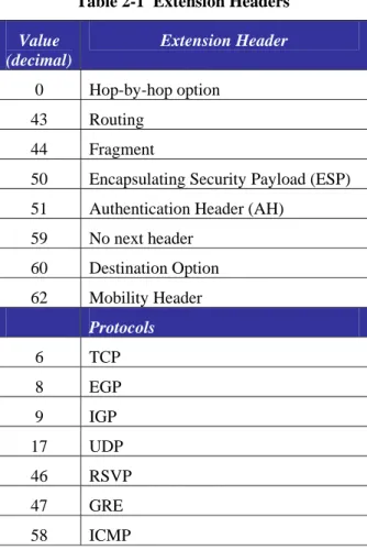
Table 2-1 Extension Headers
Value (decimal)
Extension Header
0 Hop-by-hop option 43 Routing
44 Fragment
50 Encapsulating Security Payload (ESP) 51 Authentication Header (AH) 59 No next header
60 Destination Option 62 Mobility Header
Protocols
6 TCP 8 EGP 9 IGP 17 UDP 46 RSVP 47 GRE 58 ICMP
There is one complication hidden in the header chaining mechanism: the processing of complete headers may require a walk through quite a long chain of extension headers which hinders the processing performance. To minimise this, IPv6 specifies a particular order of extension headers. Generally speaking, headers important for all forwarding nodes must be placed first, headers important just for the addressee are located on the end of the chain. The advantage of this sequence is that the processing node may stop header investigation early - as soon as it sees some extension header dedicated to the destination it can be sure that no more important headers follow. This improves the processing performance significantly, because in many cases the investigation of fixed basic header will be sufficient to forward the datagram.
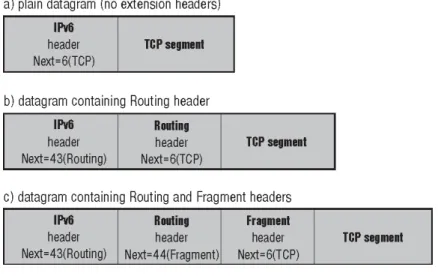
Figure 2-3 Header Chaining Examples
In the rest of this chapter we cover the most important general extension headers - options, routing and fragment. Headers related to particular mechanisms (e.g., mobility header) will be explained in their corresponding chapter.
2.3 Routing
Header
The Routing header influences the route of the datagram. It allows you to define some sequence of “checkpoints” (IPv6 addresses) which the datagram must pass through.
Two types of Routing header (identified by a field inside the extension header) have been defined: Type 0 is a general version allowing an arbitrary checkpoint sequence and type 2 is a simplified version used for mobility purposes. The definition is extensible, so more types can be added later. Let’s describe the general one first. In this case the Routing header contains two pieces of information:
1. sequence of checkpoint addresses
2. counter (named Segments Left) identifying how many of them remain to pass through
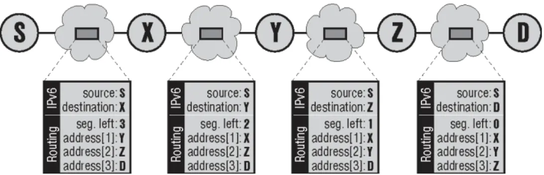
The datagram sender wanting to use this feature adds the Routing header to the datagram. It places the address of first checkpoint into the Destination address field inside the basic header. It also adds the Routing header containing the sequence of remaining checkpoints. The final datagram destination (its real target) is the last member of this sequence. Segments Left contains the number of elements in the sequence. Than the datagram is sent as usual.
When delivered to the Destination Address (actually the first checkpoint) the router finds the Routing header and realises that it is just an intermediate station. So it swaps the address in the Destination Address and the Nth address from behind of the Routing header sequence (where N is the current value of Segments Left). Segments Left is than decreased by 1 and datagram is sent to the new destination (which is the next checkpoint).
Figure 2-4 Changes in the Routing Header During Datagram Transport
The type 2 Routing header defined as a part of mobility support is a simplified version of the general type described above. It contains just one address instead of sequence of checkpoints. The general idea is following: some mobile node having a permanent address (so called home address) is travelling at present. It is connected to some strange network and obtained a temporary (care-of) address. The goal is to deliver datagrams to the care-of address, but to hide its existence from the upper layers.
So when a datagram is sent to the mobile node, the care-of address is used as the destination in basic IPv6 header. However, a routing header Type 2 is attached containing the home (permanent) address of the mobile node. When the datagram arrives at the target, the addresses are swapped and the home address is presented as the destination to upper layers.
2.4 Fragmentation
Every lower-layer technology used to transport IPv6 datagrams has some limitation regarding the packet size. It is called MTU (Maximum Transmission Unit). If the IPv6 datagram is longer than the MTU, its data must be divided up and inserted into set of smaller IPv6 datagrams, called fragments. These fragments are than transported individually and assembled by the receiver to create the original datagram. This is fragmentation.
Every fragment is an IPv6 datagram carrying part of the original data. It is equipped by a Fragment extension header containing three important data fields:
• Identification is unique for every original datagram. It is used to detect fragments of the same datagram (they are holding identical identification values).
• Offset is the position of data carried by current fragment in the original datagram.
• More fragments flag announces if this fragment is the last one or if another fragment follows. The receiving node collects the fragments and uses Identification values to group the corresponding fragments. Thanks to the Offsets it is able to put them in the correct order. When it sees that the data part is complete and there are no more fragments left (it receives the fragment identifying that no more fragments follow), it is able to reconstruct the original datagram.
The main benefit of fragmentation is that it allows the transportation of datagrams which are larger than the what the lower-layer technology can transport. The main drawback is the performance penalty. The datagram assembly at the receiver’s side is a complicated procedure requiring some buffers to collect the fragments, some timers (to limit the reassembly time and free buffers from obsolete fragments) and so on. It lowers the reliability of the datagram connection because if one single fragment is lost, whole original datagram is doomed.
• Minimum allowed MTU on IPv6 supporting links is 1280 Bytes (1500 Bytes is recommended). It decreases the need for fragmentation.
• Only the sender is allowed to fragment a datagram. If some intermediate node needs to forward it through a line with insufficient MTU, it must drop the datagram and send an ICMP message to the sender announcing the datagram drop and the MTU which inflicted it.
• Every node has to watch the path MTU for all its addressees to keep the communication as efficient as possible.
Path MTU is the minimal MTU along the route between the sender and destination of the datagram. This is the largest datagram size deliverable along the given route. Datagrams of this size should be sent if possible, because they are the most efficient (lowest overhead/data ratio).
Path MTU is based on ICMP messages announcing datagram drops due to the insufficient MTU size. The algorithm to calculate it is simple: the MTU of outgoing link is used as the first estimation. The sender tries to send a datagram of this size and if it obtains an ICMP message reporting smaller MTU, is decreases the value and tries again until the destination address is reached.
From a theoretical point of view the path MTU is flawed because the routing is dynamic, so the paths are changing and every next datagram can be delivered through a different route. In practice however, the routing changes are not so frequent. If the path MTU drops due to a routing change, the sender is informed immediately by obtaining ICMP error message and so it lowers the path MTU value.
2.5 Options
Headers containing options may provide some additional information related to the datagram or its processing. They are separated into two groups: options dedicated to every node forwarding the datagram (hop-by-hop options), and options intended for the destination host only (destination options). Table 2-2, “Hop-by-hop options” and Table 2-3, “Destination options” contain the list of defined options.
Hop-by-hop options (if present) are placed at the start of extension headers chain, because they are important for every node forwarding the datagram. The location of destination options is a bit more complicated. Actually there are two kinds of destination options: options dedicated to the final target (they are located on the end of extension headers chain) and options assigned to the next host specified by Routing header (located just before the Routing header).
Table 2-2 Hop-by-hop Options
Value Meaning
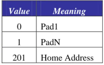
Table 2-3 Destination Options
Value Meaning
0 Pad1 1 PadN
201 Home Address
The meaning of the individual options is as follows:
Pad1, PadN
Padding. They do not carry any content, they just align the following content to the appropriate position.
Router alert
Advice to the router on content which may be important. For example RSVP sends control messages dedicated to all routers along the path, so they are equipped with a Router alert option announcing that an RSVP message is carried by the datagram.
Jumbo payload
Allows the transportation of datagrams which exceed the 64 KB maximum. The hop-by-hop option asks for special handling which is necessary to process these jumbograms.
Home Address
Chapter 3
Addressing
Rapid depletion of the available IPv4 address space was the main initiator of IPv6. In consequence, the demand to never again have to develop a new protocol due to the lack of addresses was one of the principal requirements to the new address space design. Let’s look how it was fulfilled.
The basic rules of IPv6 addressing are laid down by RFC 3513 [RFC3513]. Some accompanying RFCs define the specialties and rules for specific address types.
3.1 Addressing Essentials
The address length has been increased significantly to expand the available address space. The IPv6 address is 128 bits (or 16 bytes) long, which is four times as long as its predecessor. Because every single bit of added address length doubles the number of addresses available, the size of the IPv6 address space is really huge. It contains 2128 which is about 340 billion billion billion billion different addresses which definitely should suffice for a very long time.
Addresses are written using 32 hexadecimal digits. The digits are arranged into 8 groups of four to improve the readability. Groups are separated by colons. So the written form of IPv6 address looks like this:
2001:0718:1c01:0016:020d:56ff:fe77:52a3
As you can imagine DNS plays an important role in the IPv6 world, because the manual typing of IPv6 addresses is not an easy thing. Some abbreviations are allowed to lighten this task at least a little. Namely: leading zeroes in every group can be omitted. So the example address can be shortened to
2001:718:1c01:16:20d:56ff:fe77:52a3
Secondly, a sequence of all-zero groups can be replaced by pair of colons. Only one such abbreviation may occur in any address, otherwise the address would be ambiguous. This is especially handy for special-purpose addresses or address prefixes containing long sequences of zeroes. For example the loopback address
0:0:0:0:0:0:0:1 may be written as
::1
which is not only much shorter but also more evident. Address prefixes are usually written in the form: prefix::/length
of the address, and the “::” abbreviation is deployed. So for example prefix dedicated to the 6to4 transition mechanism is
2002::/16
which means that the starting 16 bits (two bytes, corresponding to one group in the written address) have to contain value 2002 (hexadecimal), the rest is unimportant.
Not all addresses are handled equally. IPv6 supports three different address types for which the delivery process varies:
Unicast (individual) address
identifies one single network interface (typically a computer or similar device). The packet is delivered to this individual interface.
Multicast (group) address
identifies group of interfaces. Data must be delivered to all group members.
Anycast (selective) address
also identifies a group of network interfaces. But this time the packet is delivered just to one single member of the group (to the nearest one).
Broadcast as an address category is missing in IPv6, because broadcast is just a special kind of multicast. Instead of including a separate address category, IPv6 defines some standard multicast addresses corresponding to the commonly used IPv4 broadcast addresses. For example ff02::1 is the multicast address for all nodes connected to given link.
Let’s look at the features of different address types in more detail.
3.2 Unicast
Addresses
This is the most important address type because unicast addresses are the “normal” addresses identifying the common computers, printers and other devices connected to the network.
Let’s look at the most important subtype of unicast addresses first - at the global unicast addresses defined by RFC 3587 [RFC3587]. The internal unicast address structure defined by this RFC is quite simple. It contains just three parts as depicted in Figure 3-1: global routing prefix, subnet ID, and interface ID.
Figure 3-1 Structure of the Global Unicast Address
Global routing prefix
is the network address in IPv4 parlance. This address prefix identifies uniquely the network connected to the Internet.
Subnet ID
Interface ID
holds the identifier of single network interface. Interface identifiers are unique inside the same subnet only, there may be devices holding the same interface ID in different subnets. Internet standards request the modified EUI-64 (described below) to play the role of interface ID. In reality the address structure is even more simple, because all used addressing schemes have the common length of the global prefix (48 bits) and subnet identifier (16 bits). In consequence the typical unicast address has the structure showed in Figure 3-2.
Figure 3-2 Real-world Structure of the Global Unicast Address
Not all unicast addresses are global. Some of them are limited just to a single physical (layer 2) network. These link-local addresses are distinguished by prefix fe80::/10. They can be used for intra-link communication only – both the sender and recipient of the datagram must be connected to the same local network. A router must not forward any datagram having such a destination address. Theses addresses are used in some mechanisms, such as the autoconfiguration of network parameters. RFC 3513 actually defines two scoping levels: link-local (prefix fe80::/10) and site-local (fec0::/10) addresses. But due to a long-term lack of consensus on the definition of “site” RFC 3879 [RFC3879] deprecated the usage of site-local addresses and prohibits new IPv6 implementations to handle the fec0::/10 prefix. RFC 3879 states that the given prefix is reserved for potential future usage.
Note:
Although, in theory, site-local addresses have been deprecated by RFC 3879, many IPv6 implementations and IPv6 applications still use site-local prefixes and this will probably remain true for some time. Indeed, some of the configuration examples in this book contain site-local addresses.
Consequently, unicast addresses have just two scope levels: link-local (starting with fe80::/10) or global (all the others).
3.3 Interface
Identifier – Modified EUI-64
Providing 64 bits to identify the interface in the scope of a single subnet seems to be a huge extravagance. For example 48 bits are sufficient for Ethernet addresses which are world-wide unique. Subnets for which 16 bits would not suffice to identify all the nodes are hard to imagine. On the other hand this 64-bit long interface identifier simplifies significantly some autoconfiguration mechanisms. RFC 3513 specifies the use of modified EUI-64 identifiers in this part of the IPv6 address. EUI-64 is a network interface identifier defined by the IEEE. The modification deployed in IPv6 is related to 7th bit of the 64-bit identifier. This bit distinguishes global identifiers (world-wide unique) from the local ones (unique only in the scope of single link). The value of this bit is inverted in IPv6 addresses. Hence the value 0 of this bit means a local identifier, while a value of 1 indicates a global ID.
How do we determine the value of this final part of the IPv6 address? The answer depends on the lower-layer address which the corresponding interface has. Basic rules are following:
Interface has an EUI-64 identifier
Interface has a MAC (Ethernet) address
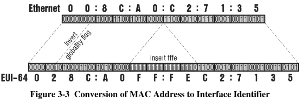
There is a simple algorithm converting the MAC address into a modified EUI-64: the global flag (7th bit) of the MAC address is inverted and the value fffe is inserted between the 3rd and 4th byte of the MAC address. For example the MAC address 00:8c:a0:c2:71:35 is converted to interface ID 028c:a0ff:fec2:7135 (the conversion is illustrated in Figure 3.3).
Otherwise
In other cases the network manager simply assigns some identifier to the interface. Typically some simple identifiers (like 0:0:0:1 and 0:0:0:2) are used. Such artificial identifiers are used for example for serial lines, which do not provide any values usable as a ground for the identification.
Figure 3-3 Conversion of MAC Address to Interface Identifier
From a technical point of view this is a perfect working mechanism. But there is a hidden drawback - a threat to privacy. Since a common computer is equipped by some MAC-addressed network card, the second rule is used for the vast majority of computers. But this means that even if the user is travelling and changing the networks used to connect to the Internet, the interface identifier of his/her computer remains constant. In other words the computer can be tracked.
RFC 3041 [RFC3041] solves this problem. It recommends the interface to have several identifiers. One of them is a fixed, EUI-64 based identifier. This is used in the “official” (DNS registered) address and is used mainly for incoming connections. The additional identifiers are randomly generated and their lifetime can be limited to a few hours or days. These identifiers are used for outgoing connections, initiated by the computer itself. Thanks to these short-lived identifiers the systematic long-term tracking of computer activities is much more difficult.
3.4 Anycast
Addresses
The essential idea behind anycast is that there is a group of IPv6 nodes providing the same service. If you use an anycast address to identify this group, the request will be delivered to its nearest member using standard network mechanisms.
An anycast address is hard to distinguish. There is no separate part of the address space dedicated for these addresses, they are living in the unicast space. The local configuration is responsible for identification of anycast addresses.
But this is not the sole problem of anycast addresses. Another problem is found in the heart of the anycasting mechanism. Selection of a particular receiver of an anycast-addressed datagram is left to IP, which means it is stateless. In consequence the receiver can change during running communication which can be truly confusing for the transport and application layers.
Yet another problem is related to security. How do we protect anycast groups from intruders falsely declaring themselves to be holders of given anycast addresses and stealing the data or sending false responses. It is extremely inadvisable to use IPSec to secure anycast addressed traffic (it would require all group members to use the same security parameters).
There is a research focused on solving the anycast problem. Until it succeeds, there are serious limitations to the anycast usage. Especially:
• Anycast addresses must not be used as a sender address in the IP datagram.
• Anycast addresses may be assigned to routers only. Anycast-addressed hosts are prohibited. In summary: anycast addresses represent an experimental area where many aspects are still researched. They are already deployed in limited scope - for example anycast address is used when a mobile node looks for home agent. The scope of this address is limited to its home network only, which makes anycast perfectly usable for such application. RFC 2526 [RFC2526] defines reserved IPv6 anycast addresses with the group span restricted to single subnet.
3.5 Multicast Addresses
Compared to anycast, multicast is a well-known entity. It is used in the contemporary IPv4 Internet, mainly to transport video/audio data in real time (e.g., videoconferencing, TV/radio broadcast). Multicast in IPv6 is just an evolution of the mechanisms already in use.
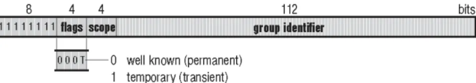
There is a separate part of the IPv6 address space dedicated to multicast. It is identified by the prefix ff00::/8. So every multicast address starts with “ff” which makes them easy to distinguish. The internal structure of the remaining 120 bits is shown in Figure 3-4.
Figure 3-4 Structure of the IPv6 Multicast Address
IPv6 multicast and multicast Addressing is discussed in more detail in Chapter 8.
3.6 Required
Addresses and Address Selection
There is a serious difference between IPv4 and IPv6. Every interface has just a single address in IPv4. If you want to assign more addresses to the same interface, you have to use various hacks (i.e., virtual sub-interfaces) or vendor specific implementations that do not adhere to open standards such as DHCP.
functionality. Required addresses for a common host (computer, printer or any other device which does not forward the datagrams) are as follows:
• link-local address for every interface
• assigned (configured) unicast and multicast addresses for the interfaces
• loopback address (::1)
• all-nodes multicast addresses (ff01::1, ff02::1)
• solicited node multicast address
• assigned multicast addresses (identifying groups to which the node belongs)
For example a PC equipped with a single Ethernet network card having a MAC address of 00:2a:0f:32:5e:d1 sitting in two subnets (2001:a:b:c::/64 and 2001:a:b:1::/64) and participating in the group ff15::1:2:3 must receive data on all these addresses:
• fe80::22a:fff:fe32:5ed1 (link-local)
• 2001:a:b:c:22a:fff:fe32:5ed1 (configured unicast)
• 2001:a:b:1:22a:fff:fe32:5ed1 (another configured unicast)
• ::1 (loopback)
• ff01::1 (all nodes on the interface)
• ff02::1 (all nodes on the link)
• ff02::1:ff32:5ed1 (solicited node multicast)
• ff15::1:2:3 (configured multicast)
A router has even more required addresses. It must support all the addresses obligatory for a node plus:
• anycast address for all routers in the subnet for every interface on which it acts as a router
• all assigned anycast addresses
• all-routers multicast (ff01::2, ff02::2, ff05::2)
Suppose that the aforementioned node is a router. It operates as a home agent (see Chapter 10 about mobility for the description of this) in both subnets, so it should listen to the corresponding all-home-agents anycast addresses. In this case it must in addition to addresses already stated support:
• 2001:a:b:c:: (routers in first subnet)
• 2001:a:b:1:: (routers in second subnet)
• 2001:a:b:c::fdff:ffff:ffff:fffe (home agents in first subnet)
• 2001:a:b:1::fdff:ffff:ffff:fffe (home agents in second subnet)
• ff01::2 (all routers on the interface)
• ff02::2 (all routers on the link)
• ff05::2 (all routers in the site)
RFC 3484 [RFC3484] brings the rules for this situation. It defines an imperative algorithm to select the sender and receiver addresses for an IP datagram. The general idea behind the address selection is following. The application willing to communicate will call some system service (typically the getaddrinfo() function) to obtain a list of available addresses for given target host. It takes the first of these addresses, selects some appropriate source address and tries to establish the communication. In the case of failure the next potential destination address from the list is used.
We do not cover the exact rules to judge between addresses here because they are important for the implementers of IPv6, not for its users. But one aspect of these rules should be mentioned here – the policy table.
It is a dedicated data structure used to express relationships (affinity) between addresses. Every entry of the policy table contains: address prefix, precedence and label. When evaluating some address, the entry containing longest matching prefix is used to assign the precedence and label to the address. Generally speaking: two addresses (source and destination) having the same label are related which increases their chance to be selected.
Using the policy table you may influence the address selection algorithm by assigning labels to particular prefixes. Of course it is not obligatory, there is a default policy table defined by RFC 3484 which will be used in such case.
3.7 Real-world
Addresses
Leaving aside the addressing ‘theory’, in reality the IPv6 address space has been partitioned into a few areas which have a fixed meaning. You can see the allocation in Table 3-1.
Table 3-1 IPv6 Address Allocation
::0/128 Unspecified address ::1/128 Loopback address ff00::/8 Multicast addresses fe80::/10 Link-local addresses
fec0::/10 Deprecated (former site-local addresses) other Global unicast addresses
The vast majority of the address space is occupied by global unicast addresses. But just a tiny part of this allocation is really used – no more than three /16 prefixes (see Table 3-2, “Global unicast prefixes in real use”).
Table 3-2 Global Unicast Address Prefixes in Use
2001::/16 Regular IPv6 addresses 2002::/16 6to4 addresses
The 2002::/16 prefix is dedicated to 6to4 mechanism allowing automatic tunnelling of IPv6 datagrams over common IPv4 Internet (described later in this book). The 3ffe::/16 prefix was used in the 6bone network – an experimental overlay network intended to gain practical experience with IPv6 operation. Allocations from this address space have been stopped. The support (routing) of these addresses will be deprecated at the end of June 2006 (RFC 3701 describes the 6bone phase-out schedule). In consequence the usage of 3ffe::/16 prefix drops and many 6bone addresses have already been abandoned.
The most important address prefix is the 2001::/16 from which all the regular global unicast addresses in the contemporary Internet originate. Allocation of addresses from this prefix is managed by Regional Internet Registries (RIRs) – the same organisations which also manage the IPv4 address space.
Every RIR has obtained some part of the 2001::/16 prefix from which it allocates smaller parts. Regions covered by a single RIR are quite large (e.g. a continent), so the allocation is not made directly. It is made in collaboration with Local Internet Registries (LIRs), which are typically the Internet providers. The mechanism is similar – every LIR obtains some part of the address space from which it allocates prefixes to its customers.
All the RIRs have agreed on common allocation rules and the address structure displayed in Figure 3-5. This clear and well-arranged structure is the result of a few years of evolution. One of the really nice features of this contemporary addressing structure is that the borders between different authorities are situated at the colons in the address written form.
The first four hexadecimal digits are fixed, they are 2001. The next four are assigned by the RIRs. It means that if some LIR asks for an address space to manage it obtains a 32-bit prefix from which 48-bit prefixes are allocated to its customers (end-sites). So the specification of the third quadruple is up to the LIR. Finally, the last foursome of hexadecimal digits in the first half of the address contains the subnet ID. This is assigned by the local network manager.
Figure 3-5 Structure of the Real-world Global Unicast Address Prefix
Let’s look at an example: CESNET is the operator of Czech National Research and Education Network and also the LIR serving organisations connected to this network. CESNET obtained from RIPE NCC (RIR responsible for Europe) the prefix 2001:718::/32. /48 prefixes from this space are assigned to institutions connected to the CESNET network – for example the Czech technical University in Prague obtained the prefix 2001:718:2::/48. Its subnet number 1 has the prefix 2001:718:2:1::/64.
It is possible for the address holder to define some hierarchy of addressing scheme in the address part for which it is responsible. For example the end-site can specify the rules to assign subnet IDs. Say that the network is spread around few buildings. Natural hierarchy in this case could be to use the first part of subnet ID to identify the building and the rest to distinguish particular LANs inside the same buildings.
If you decide to deploy such a hierarchy, it is tempting to say “First N bits is the building identifier, the remaining 16–N bits identify the subnets inside building.” RFC 3531 recommends not to do so, because later you may decide that your estimation about future network development was bad and some part of the hierarchy does not suffice for the network growth.
0...0001 (0001), the second is 0...0010 (0002), the third 0...0011 (0003), etc. When combined for example 4003 means third LAN in second building. This opposite growth ensures the postponement of part-border assignment up to the moment when the growing lengths of both parts meet. You may then find that instead of the planned division of bit 8:8 for building and LAN identifiers, the real need is to use 6:10.
Similarly the LIR can define some system in the third quadruple to assign /48 prefixes to customers. For example the first part may identify the node (point of presence), the second one distinguishes customers connected to the same node. The IPv6 addressing structure provides freedom for such decisions. The hierarchy inside individual parts marked in Figure 3-5 is not strictly defined by the RFCs, nor prohibited. It is up to the manager of the corresponding part to develop the rules. In most cases these rules are just internal, they are not communicated to the customers.
And finally we should answer the Big Principal Question: “How to get IPv6 addresses for my network?”
The answer is that it depends on your position in the addressing “food chain”. If you are an end-customer, simply ask your IPv6 connectivity provider. The correct answer would be to ask the corresponding LIR, but the provider and LIR are usually the same body. You should get a 48-bit prefix. If the provider tries to assign you some longer prefix (smaller address space), argue and fight for /48, because RFC 3177 clearly states that /48 should be the standard network prefix length for almost all networks.
If you are a LIR and would like to provide IPv6 addresses to your customers, your situation is more complicated. You must ask your RIR to assign you some part of the address space. It is done the usual way – by filling in an application form. But there are some requirements which you have to meet to qualify for getting some address space. In the time of writing this text the requirements are:
• You have to be a LIR.
• You must not be an end site.
• You must develop a plan to provide IPv6 connectivity to connected sites. You have to assign /48 prefixes to these sites and aggregate all these prefixes to a single routing table entry used to advertise your network to the rest of world.
• You have to have a plan for assign at least 200 prefixes to other organisations within two years.
Chapter 4
Essential Functions and Services
This chapter looks at what we consider to be ‘essential’ functions and services of IPv6. In other words, without these functions and services we would not be able to achieve satisfactory IPv6 operation (or even no connectivity at all). First, we briefly describe Neighbour Discovery and look at several router configurations. Next we detail how DNS works in IPv6 and describe how this worked in the 6NET network. Finally, we describe DHCPv6 along with several available implementations.
4.1 Neighbour
Discovery
Neighbour discovery is a protocol that allows different nodes on the same link to advertise their existence to their neighbours, and to learn about the existence of their neighbors. It is a basic functionality all implementations of IPv6 on any platform must include.
Neighbor discovery for IPv6 replaces the following IPv4 protocols: router discovery (RDISC), Address Resolution Protocol (ARP) and ICMPv4 redirect.
Neighbor discovery is defined in the following documents:
• RFC 2461, Neighbor Discovery for IP Version 6 [RFC2461]
• RFC 2462, IPv6 Stateless Address Autoconfiguration [RFC2462]
• RFC 2463, Internet Control Message Protocol (ICMPv6) for the Internet Protocol Version 6 Specification. [RFC2463]
RFC 2461 and 2462 are currently in the process of being revised by the IPv6 working group of the IETF. These drafts [RFC2461bis], [RFC2462bis] will eventually replace the older RFCs.
The combination of these protocols allow IPv6 hosts to automatically detect the presence of other hosts on the link including, of course, the presence of on-link routers. From the messages sent by routers, IPv6 hosts can automatically configure themselves with appropriate addresses and other state necessary for operation. Neighbour Discovery mandates duplicate address detection so that a host cannot try to use an IPv6 address already in use by another host on the link and also allows a host to detect when another host on the link becomes unreachable.
Neighbor discovery uses the following Internet Control Message Protocol Version 6 (ICMPv6) messages:
• router solicitation (RS)
• router advertisement (RA)