Collateralised Debt Obligations
Domenico Picone
1City University Business School, London
Royal Bank of Scotland
Abstract
This chapter explores the market of CDOs and synthetic CDOs and their use in bank balance sheet management. We first review different types of CDOs used in capital markets and their economic rationals and then discuss the growth in synthetic CDOs under structural and balance sheet management perspectives. Following this we analyse the CDO equity piece and how it can be used in portfolio management, and then, we offer a structuring example: using with the Moody’s Binomial Expansion
and Double Binomial Expansion Techniques we arrive at the best debt structure for
a synthetic CDO. We conclude with a short introduction on the S&P CDO evaluator.
1
The CDO structure
A CDO is a special purpose company or vehicle (SPV), complete with assets, liabilities and a manager.
Typically, the CDO’s assets consist of a diversified portfolio of illiquid and credit-risky assets such as high yield
bonds (CBO) or bank leverage loans (CLO)2.
Figure 1: CDO Diagram
We have set up a typical CDO structure in Figure 1. The assets are transferred to the SPV that funds these assets, from cash proceeds of the notes it has issued.
The CDO structure allocates interest income and principal repayment from a pool of different debt instruments to a prioritised collection of securities notes called tranches.
Senior notes are paid before mezzanine and lower rated notes. Any residual cash flow is paid to the equity piece. This makes the senior CDO liabilities significantly less risky than the collateral.
1
The content of this paper reflects personal view of the author and not the opinion of Royal Bank of Scotland.
2
Most recently, CDO technology has been extended to emerging market debts, structured finance securities, commercial real estate-linked debt, distressed assets, and last to arrive, private equity funds.
On every payment date, equity receives cash distributions after the scheduled debt payments and other costs have been paid off. The equity is also called the “first-loss” position in the collateral portfolio. This is because it is exposed to the risk of the first dollar loss in the portfolio.
The CDO rating is based on its ability to service debt with the cash flows generated by the underlying assets. The debt service depends on the collateral diversification and quality guidelines, subordination and structural protection (credit enhancement and liquidity protection).
As we move down the CDO’s capital structure, the level of risk increases. The equity holders that bear the highest risk have the option to call the transaction after the end of the non-call period, which in most cases lasts three to five years.
The typical CDO consists of a ramp -up period, during which the collateral portfolio is formed, a reinvestment period, during which the collateral portfolio is actively managed, and an unwind period, during which the liabilities are repaid in order of seniority using collateral principal proceeds.
During the reinvestment phase, the equity class distributions consist of excess interest on the full portfolio, minus collateral interest income remaining after the payment of debt interest and other fees. The manager would reinvest collateral principal proceeds.
In the repayment period, excess interest payments gradually decrease as the collateral portfolio principal proceeds are used to repay the debt in order of seniority. After all the debt classes have been redeemed, and if the equity class has not elected to call the transaction, the remaining principal payments pass to the equity.
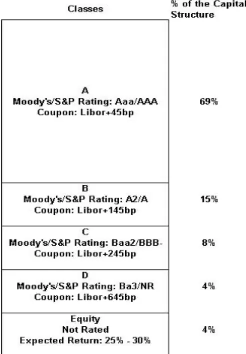
Figure 2 displays an example capital structure, where the high yield bonds collateralise CDO liabilities.
1.2 Arbitrage and Balance Sheet CDOs
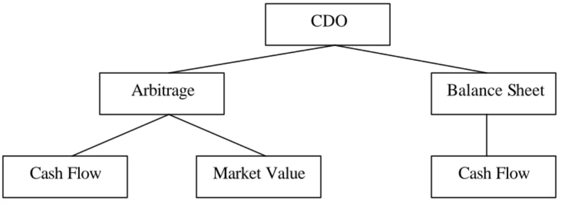
Most CDOs can be placed into either of two main groups: arbitrage and balance sheet transactions. Figure 3 shows the conceptual breakdown between the two structures.
Figure 3: CDO structure
• Cash flow CDOs
A cash flow CDO is one where the collateral portfolio is not s ubjected to active trading by the CDO manager. The uncertainty concerning the interest and principal repayments is determined by the number and timing of the collateral assets that default. Losses due to defaults are the main source of risk.
• Market value CDOs
A market value CDO is one where the performance of the CDO tranches is primarily a mark -to-market performance, i.e. all securities in the collateral are marked to market with high frequency.
Market value CDOs leverage the performance of the asset ma nager in the underlying collateral asset class. As part of normal due diligence, a potential CDO investor needs to evaluate the ability of the manager, the
institutional structure around him, and the suitability of the management style to a leveraged inves tment vehicle.
• Balance sheet cash flows CDOs
Balance sheet deals are structures for the purpose of capital relief, where the asset securitised is a lower yielding debt instrument. The capital relief reduces funding costs or increases return on equity, by removing, the assets that take too much regulatory capital, from the balance sheet.
These transactions rely on the quality of the collateral that is represented by guaranteed bank loans with a very high recovery rate.
The relative low coupon attached to these assets, results in a smaller spread cushion than the corresponding arbitrage structure. However, given their relative superior quality, they require less subordination when used in a CDO deal.
In the majority of the cases, the sold assets are loan-secured portfolios.
The size of a typical balance sheet CDO is in general very large, as the transaction must have an impact on the ROE of the institution looking for capital relief.
CDO
Arbitrage
Balance Sheet
• Arbitrage CDOs
The aim of Arbitrage CDOs is to capture the arbitrage opportunity that exists in the credit-spread differential, between the high yield collateral and the highly rated notes.
The idea is to create a collateral with a funding cost lower than the returns expected from the notes issued. Most arbitrage deals are private ones, where size is not large and the number of assets included in the deal are very limited compared to the cash flow type.
• Arbitrage market value CDOs
Arbitrage market value CDOs, unlike balance sheet CDOs where there is no active trading of loans in the portfolio, go through a very extensive trading by the collateral manager, necessary to exploit perceived price appreciations.
This type of CDO relies on the market value of the pool securitised, which is monitored on a daily basis. Every security traded in capital markets, with an estimated price volatility, can be included in this type of CDO. In fact, the primary consideration is the price volatility of the underlying collateral.
The important aspect is the collateral manager’s capacity to generate a high total rate of return. The CDO manager has a great deal of flexibility in terms of the asset included in the deal. During the revolver period, the collateral manager can increase or decrease the funding amount that changes the leverage of the structure.
• Arbitrage cash flow CDOs
By their very nature, collateral assets have been purchased at market price and are negotiable instruments, therefore most assets are bonds. However syndicated loans, usually tradable, have been included in past transactions. As arbitrage deals, the collateral assets can be refinanced more economically by re -tranching the credit risk and funding cost in a more diversified portfolio. Unlike arbitrage market value CDOs, the collateral assets are not traded very frequently.
1.3 Credit enhancement in cash flow transactions
Senior notes in cash flow transactions are protected by subordination, over-collateralisation and excess spread.
The senior notes have a priority claim on all cash flows generated by the collateral, therefo re, non-senior notes’ performance is subordinated to the good performance of senior notes.
Over-collateralisation provides a further protection to senior notes by imposing a minimum collateral value with two coverage tests: par value and interest coverage tests.
Par value test requires that the senior notes (and subsequently the other notes) are at least a certain percentage of the underlying collateral (for example 115%).
The par value test is applicable to lower rated notes (mezzanines). In this case, t he trigger percentage below that fails the test is selected at a lower rate (for example 105%).
An interest coverage test is applied to ensure that collateral interest income is sufficient to cover losses and still make interest payment to the senior notes . This credit support is also known as excess spread.
Credit enhancement may also be in the form of a letter of credit from a highly rated institution, a cash collateral account, or a guarantee.
1.4 Credit enhancement in market value transactions – Advance rates and the OC test
Advance rates are the primary form of credit enhancement in market value transactions.
The advance rate is the maximum percentage of the market rate that can be used to issue debt. Rating agencies assign different advance rates t o different types of collateral. They depend on the volatility of the asset return, and on the liquidity of the asset in the market. Assets with a higher return volatility and lower liquidity are given lower advance rates.
Table 1 shows a sample table that Fitch would apply to different asset classes.
For example, it is possible to issue AA debt with 95% of the market value of CD or CP as collateral asset. To
issue BB debt, we could use 100% of the market value of the same instrument.
Asset Category AA A BBB BB B
Cash and Equivalents 100% 100% 100% 100% 100%
CD and CP 95% 95% 95% 100% 100%
Senior Secured Bank Loans 85% 90% 91% 93% 96%
BB-High Yield Debt 71% 80% 87% 90% 92%
<BB-High Yield Debt 69% 75% 85% 87% 89%
Convertible Bonds 64% 70% 81% 85% 87%
Convertible Preferred Stock 59% 65% 77% 83% 86%
Mezzanine Debt, Distressed, Emerging Market 55% 60% 73% 80% 85%
Equity, Illiquid Debt 40% 50% 73% 80% 85%
Source: Fitch
Table 1: Fitch’s Advance Rates
For market value transactions, there are usually multiple Over-collateralisation tests.
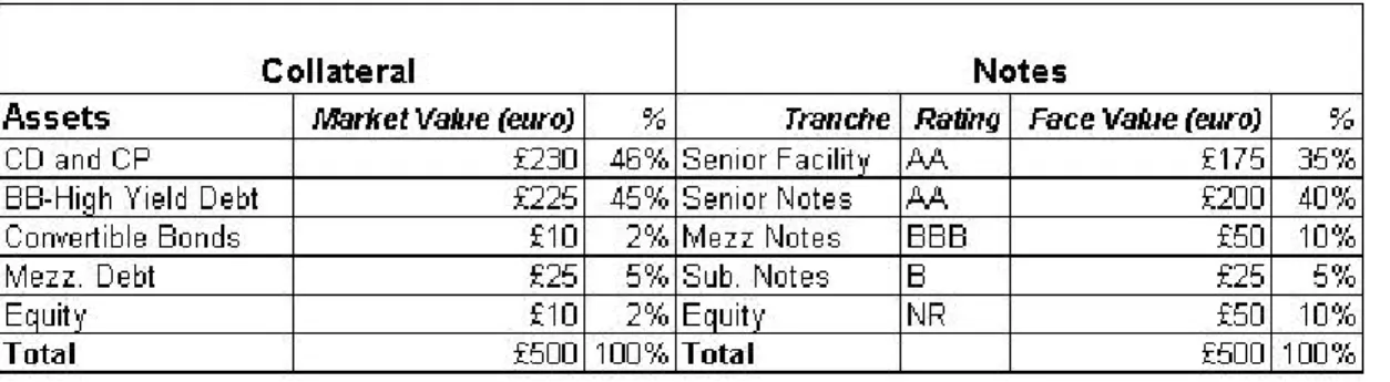
To illustrate how the test works, we introduce a simple example with the collateral and liability structure of Table 2
Table 2: CDO market value transaction
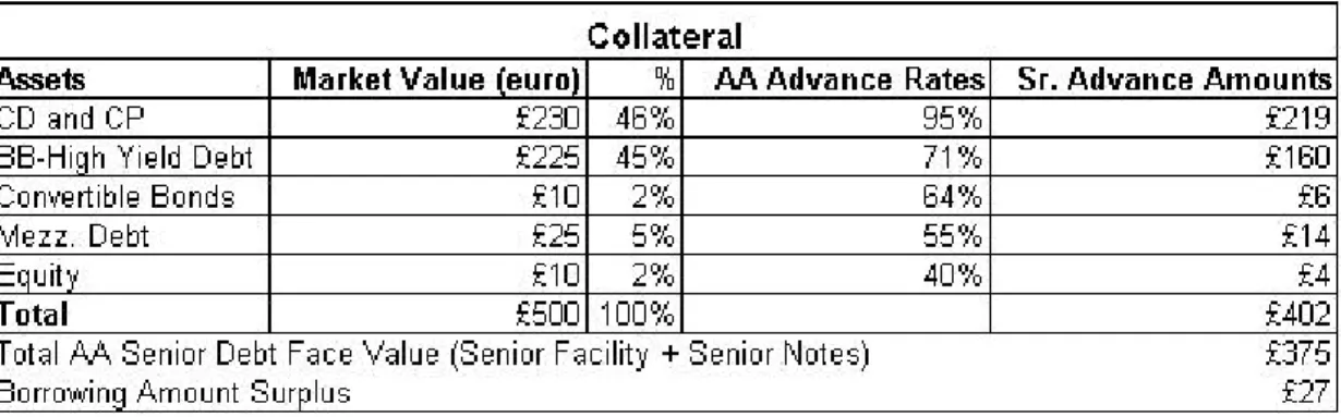
After applying the AA advance rates, we can see from Table 3 that the senior advance amount exceeds the total
AA debt, defined as Borrowing Amount Surplus, by £27 m. This is also the market value loss that the AA
Table 3: AA Debt OC test
Tables 4 and 5 show respectively, the borrowing amount surpluses of the AA+BBB debt and the AA+BBB+B
debt. As for Table 3, the borrowing amount surpluses of 23 and 25 are the market value losses that the AA+BBB
and AA+BBB+B structures can respectively sustain before breaching their OC tests.
Table 4: AA+BBB Debt OC test
Table 5: AA+BBB+B Debt OC test
A collateral manager must ensure that the market value tests are not violated due to fluctuations in the underlying prices. A breach of the OC test is quite serious, and when it happens, the collateral manager must remedy it within a cure period that is usually between two to ten business days.
There are usually two options:
• or to sell security/ies with a lower advance rate and repay the debt starting with the more senior notes. The first action is preferred when the OC test is slightly out of compliance. The second is a drastic cure. If the collateral manager cannot comply with the OC test, the debt holders have the power to take control of the fund and liquidate the portfolio in an event of default.
1.5 Credit enhancement in market value transactions – Minimum Net Worth test
The Minimum net worth test is also designed to offer credit protection to the senior notes holders, by creating an equity cushion. This is achieved by imposing that the excess market asset value, minus the debt notes is equal or greater than the equity face value, times a percentage
MAV - Debt >= % * Equity.
In cases where the test is breached, the manager has a cure period to bring the CDO into compliance, by either
• redeeming part or all of the senior notes,
• by generating enough capital gains by selling some assets.
The latter is preferable since the manager would not de-leverage the deal.
If the collateral manager cannot comply with the minimum net worth test, and an event of default occurs, the debt holders have the power to call the deal.
1.6 The Manager
The manager of the CDO is responsible for the credit performance of the collateral portfolio and for ensuring that the transaction meets the diversification, quality and structural guidelines specified by the rating agencies. In return for managing the collateral portfolio, the manager receives a fee, typically divided into base and incentive components. During the reinvestment period, the CDO manager continuously evaluates the state of the collateral portfolio and of the overall market. He trades out positions at risk for credit deterioration, and takes advantage of appreciation opportunities.
The key to a successful market value CDO is the manager’s ability to generate high risk-adjusted returns through research, market knowledge and trading ability. The return performance of CDO equity hugely depends on the long-horizon returns of the underlying portfolio realised by the manager.
Today, successful CDO management franchises are found in a variety of asset management organisations, including mutual fund groups, insurance companies, banks, private equity firms and hedge funds.
Different managers stress different strategies to generate high risk-adjusted returns. For example, an insurance company may depend on its portfolio risk management system, a mutual fund group may use its size and market knowledge, and a private equity sponsor may rely on its knowledge of leveraged companies. The market value CDO is typically only open to managers who have established track records and who have demonstrated a high level of organisational commitment to the CDO business. Most successful CDO managers consider CDO issuance to be an integral component of their overall business development strategy.
CDOs are also a powerful asset-gathering tool that locks in management mandates for a fixed term, providing managers with exposure to a larger and more diverse pool of investors. For example, a traditional high-yield
manager will form relationships with asset-backed AAA investors such as banks or structured investment vehicles, BBB buyers such as insurance companies, and alternative investment buyers who purchase the equity. In this way, broader client exposure helps the growth of the overall management franchise, without straying from core competency.
Additionally, by locking the structure to a financing rate and fixed term, the manager is free to focus exclusively on long-term horizon management rather than worry about short -term liquidity issues.
Although during the pay down phase of the CDO, the manager’s abil ity to reinvest principal proceeds is limited, the manager is still responsible for avoiding problem credits in the portfolio.
2
The Economic rational for CDOs
CDOs make most economic sense for collateral securities in markets where there is limited information (inefficient) with the possibility of high risk-adjusted returns through active management.
Risky assets, such as the debt of leveraged corporations, are often difficult to analyse and value, thus limiting their potential investor base and creating a gap in the economy between the demand and supply of risky finance. As result, corporate debts are relatively illiquid in the secondary market.
The CDO structure addresses this market inefficiency by bringing a specialised manager to the transaction and allocating much of the risk, in the form of a liquidity premium in the equity class.
The CDO cash flow structure acts as a cushion and hedges the debt from defaults and the direct impact of mark -to-market changes in the value of the collateral.
In trying to reach its economic target, an issuer would have two main constraints: to minimize the total cost of notes (i.e. the floating or fixed rate attached to each note) and to minimize the size of the subordinated notes (among them the equity piece).
Normally, the seller would retain 2% of the structure, the first loss, by keeping the equity piece. He would also
fund the Cash Collateral Account (CCA), a cash deposit that re -enforces the credit protection, usually in the range of 1% of the structure.
The originator’s return is given by the excess spread of the notes (average rate of the loan portfolio minus the average rate of the notes) over the funding cost of his collateral. His maximum loss is also known and given by the first loss.
Figure 4 shows an example of ROE before and after a CDO.
Figure 4: Regulatory Capital relief and ROE
In the example of Figure 4 the bank has a portfolio of loans of 100 million Euros on its balance sheet (left box), for which the average spread over the Libor is 100 bps. The loans receive a risk weight of 100% where the Regulatory Capital is 8%, and the loan portfolio ROE is of 12.5%.
With the CDO structure in Figure 4 (right box) the bank retains only 2% of the original loan portfolio (the loss piece) and securitises the remaining 98%. In this example, the bank would receive a huge relief of regulatory
capital. This would drop from 8 million euros to 2 million euros. The new ROE is 32.8%3. If this transaction
had a bigger volume it would hugely affect the ROE of the overall bank.
Alongside this, the bank would continue its commercial activity on its lending portfolio, and would carry out a review of its IT and scoring systems.
3
This is calculated by dividing the gross return from the loan portfolio of 100 bps minus the average cost of the three notes (100 bps – 34.4 bps) by 2, which is the amount of regulatory capital.
3
Synthetic Collateralised Synthetic Obligations
In most conventional cash flow CDOs, assets are actually transferred into the SPV. However, the process of
transferring loans to the SPV requires significant up front work. A loan-by-loan analysis is necessary to check it complies with the securitisation programme and to verify that there are no special clauses attached to any loan limiting its transfer.
The first stage of evolution of the conventional CDO, arrived when the credit risk was transferred into the SPV
through a credit default swap4, and when the underlying credit ownership of the underly ing pool remained in the
originator’s book. For this the term synthetic is used, since the risk was synthetically transferred out of the
originator’ balance sheet.
With synthetic CDO’s, the big advantage is that sensitive client relationship issues arisin g from loan transfer notification, assignment provisions and other restrictions can be avoided. Also, client confidentiality can be maintained. Not to mention that it takes less time to complete the transaction.
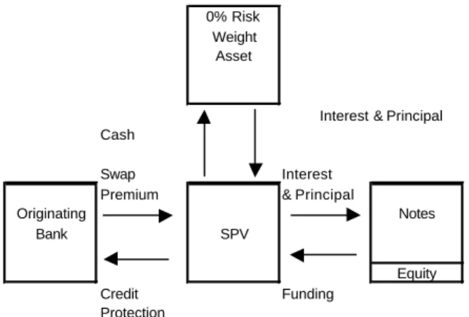
3.1 Fully funded synthetic structures
Historically, the fully funded CDO was the first to be used as an alternative to the more traditional structure. In a fully funded synthetic CDO, the SPV issue notes for approximately 100% of the reference portfolio. The proceeds of these notes are generally invested in high quality securities used as collateral that have a 0% risk weight.
In order to hedge its credit risk exposure in its loan portfolio, the originating bank enters into a Credit Default Swap (CDS) with either the same SPV or with an OECD bank. With the CDS the originator buys credit protection in return for a premium.
The premium received is then added to the interest notes received by the note investors. The mechanics are described in the Figures 5 and 6.
0% Risk Weight
Asset
Interest & Principal Cash
Swap Interest
Premium & Principal
Originating Notes
Bank SPV
Equity
Credit Funding
Protection
Figure 5: Fully funded synthetic CDO with CDS with an SPV
4
Swiss Bank brought Glacier Finance 1997-1 and 1997-2 to market in late 1997. This was a master trust structure where Swiss Bank transferred the credit risk via a portfolio of credit linked notes.
0% Risk Weight
Asset
Interest Cash & Principal
Swap Swap Interest
Premium Premium & Principal
Originating OECD Notes
Bank Bank SPV
Equity
Credit Credit Funding
Protection Protection
Figure 6: Fully funded synthetic CDO with CDS with an OECD bank
The equity retained by the originator brings a 100% risk weight. Therefore, as with the example in Figure 5, the bank would achieve a first capital release of 6%. An additional regulatory capital would depend on the presence of an OECD bank in the structure.
If the CDS is directly with the SPV (Figure 5), and if the note proceeds are invested in 0% risk weighted assets, no more regulatory capital is added to the transaction.
If the CDS is directly with an OECD bank (Figure 6), the regulatory capital on the CDS is 1.6% (i.e. 20% * 8%) of the notional amount of the same swap.
If the CDS has a notional equal to reference portfolio the total regulatory capital charge of this transaction would be 3.6%.
3.2 Partially funded structures
In fully funded CDOs, the bank originator is far from achieving an efficient capital use. Fully funded CDO-CLO
may sometimes be a relatively expensive programme. However, it is also true that as term funding debt, a
CDO-CLO programme remains less exposed to the risk that credit spreads may widen.
The structure behind a partially funded CDO transaction is very similar to that of a fully funded one. The originator bank buys credit protection d irectly from an SPV (Figure 7) or from an OECD bank (Figure 8). The difference is that the SPV issues a lower amount of notes because it guarantees a lower amount of collateral.
What really characterises this structure is the un-funded piece called the Super Senior. This is a very high
quality financial paper, virtually with a zero probability of being exposed to a credit loss.
The originating bank enters in a CDS (super senior CDS) with an OECD bank for the amount of the super senior tranche.
Super Senior CDS
0% Risk Weight
Asset Swap
Reference Originating Premium OECD
Loan Bank Bank Interest
Portfolio & Principal
Unfunded Credit
Protection Interest
& Principal Reference
Loan Originating Swap Premium SPV Notes
Portfolio Bank
Funded Credit Protection Equity
Funding
Junior CDS
Source: Investing in Collateralized Debt Obligations, Frank J. Fabozzi, Laurie S. Goodman Figure 7: Partially funded synthetic CDO with CDS with an SPV
Super Senior CDS
0% Risk Weight
Asset Swap
Reference Originating Premium OECD
Loan Bank Bank Interest
Portfolio & Principal
Unfunded Credit
Protection Interest
& Principal
Reference Swap Swap
Loan Originating Premium OECD Premium SPV Notes
Portfolio Bank Bank
Funded Equity
Credit Credit Funding
Protection Protection
Junior CDS
Source: Investing in Collateralized Debt Obligations, Frank J. Fabozzi, Laurie S. Goodman Figure 8: Partially funded synthetic CDO with CDS with an OECD bank
The treatment of regulatory capital for European banks is currently still different from jurisdiction to jurisdiction.
The Federal Reserve Bank has issued several interpretations that apply only to US banks. Some conditions are necessary to receive a better treatment of regulatory capital. If these conditions are met, and if the credit risk is transferred to another OECD bank with a CDS, the super senior piece receives a risk weight of 20% with the capital charge of 8%.
The regulatory capital rules on the equity piece and on the junior CDS, are the same as those applied on the fully funded CDO’s. Therefore, the last step is to add the regulatory capitals required on the funded and un -funded part of the structure.
If we apply those percentages to the portion of the super senior piece (87%), the total regulatory capital is 3.4% (4% for the Super Senior CDS and 2% for the Equity piece).
3.3
Balance Sheet Management with CDS
All banks constantly seek least expensive funding cost. Therefore, it does not come as a surprise that banks have a preference towards partially funded programmes.
If we compare Figure 8 with 1, the difference in funding between the two structures becomes clear. An example makes this even clearer.
Figure 10: Funding costs with a fully and partially funded synthetic CDO
Figure 10 contains the CDO structure of Figure 5, plus a new and more convenient structure for the originator: partially funded CDO.
With the partially funded structure, we have achieved a reduction of the funding cost: the overall transaction
cost has dropped by 9 bps5. Furthermore, for one unit of equity used in the partially funded structure, the
originator would pay 7.26 bps Vs 17 bps for the fully funded.
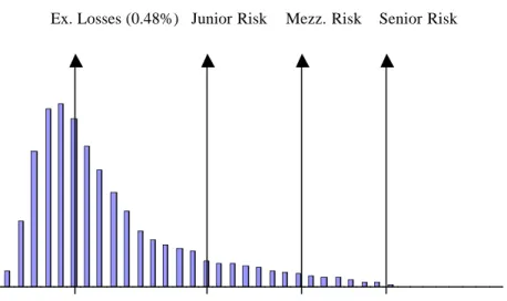
Assuming now that all the loans in Figure 5 are Baa1 loans, with a maturity of 6 years, a cumulative default
probability of 37%6 and a recovery rate of 65%, the expected loss on this portfolio is 0.48% = (1-65%)*37%.
Consequently, the expected losses have to rise by a factor of four before hitting the junior notes. The Figure 11 shows the statistical distribution of losses that might occur on this transaction.
5
(34 bps – 25 bps) = 9 bps
6
Ex. Losses (0.48%) Junior Risk Mezz. Risk Senior Risk
1
Figure 11: Distribution of Expected Losses
The structure is also free of any interest rate mismatch, i.e. it pays Libor and receives Libor.
The average spread of 100 bps compensates the bank for taking the credit risk of expected losses. The credit spreads, ranging from 25 to 200 bps, compensate the notes investors for taking different risks.
Therefore, we can remove the Libor and leave the spreads only as in Figure 12.
Assets % Spreads Liabilities % Spreads
Loan 1 2% 100 bps Super Senior Notes 87% 15 bps
Loan 2 2% 100 bps Senior Notes 3% 25 bps
Loan 3 2% 100 bps Mezzanine Notes 4% 80 bps
………. … 100 bps Junior Notes 4% 200 bps
Loan 50 2% 100 bps Retained Equity 2% Dividend
CDO Structure
Figure 12: CDO structure with hedged interest rate risk
In general terms, a CDS is designed to mimic the credit behaviour of a floating rate note, such as the loans in Figure 12. The loan spread, that is constant until the loan matures, is equivalent to the fixed leg of a CDS. In fact, the CDS seller, who seeks credit exposure, receives X basis points, i.e. a spread, per year until the credit reference matures or defaults. The constant spread is the fixed leg of the CDS.
As a consequence, we can remove the loans and add the CDS on the asset side.
Assets % Spreads Liabilities % Spreads
CDS 1 2% 100 bps Super Senior Notes 87% 15 bps
CDS 2 2% 100 bps Senior Notes 3% 25 bps
CDS 3 2% 100 bps Mezzanine Notes 4% 80 bps
………. … 100 bps Junior Notes 4% 200 bps
CDS 50 2% 100 bps Retained Equity 2% Dividend
CDO Structure
With the CDO in Figure 13 the bank is now exposed to the credit risk of 50 synthetic assets. To hedge its position, the bank borrows via four different credit r isk notes. Retaining the equity, gives it the right to a possible dividend.
Some of the loans in Figure 13 may be in the same industry and same country. Thus, it is safe to assume that they may be affected by the same risk factors. As a consequence, we may treat them as one loan with a notional equal to the sum of their notionals.
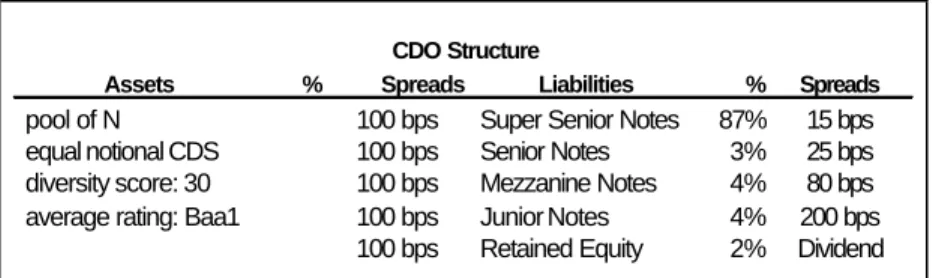
Assets % Spreads Liabilities % Spreads
pool of N 100 bps Super Senior Notes 87% 15 bps equal notional CDS 100 bps Senior Notes 3% 25 bps diversity score: 30 100 bps Mezzanine Notes 4% 80 bps average rating: Baa1 100 bps Junior Notes 4% 200 bps
100 bps Retained Equity 2% Dividend
CDO Structure
Figure 14: CDO structure with a basket CDS
Figure 14 shows, on the asset side, a basket CDS with equal notional and a diversity score of 30, on a reference
pool with average rating of Baa1.
The Diversity Score in Figure 14 indicates that the 50 loans almost behave as 30 uncorrelated loans.
Viewed from this angle, a CDO is a hedged portfolio. The assets are a portfolio of synthetics, the liabilities are the tranches with different ratings. By hedging its balance sheet from credit risk (and from interest rate risk), the bank is trying to achieve a higher return than investing in risk-less treasury bonds. By partially funding the CDO structure, the bank has also achieved a leverage position, with potentially huge returns.
5
Valuing a CDO
There are several factors that affect the value of all CDO tranches (debt and equity pieces).
But the most important is the credit quality of the underlying portfolio, which depends on the individual securities’ default probabilities and diversification.
Improvement or deterioration in the credit quality of collateral securities has a pronounced impact on the equity, since it represents a leveraged position.
Changes in the level of portfolio diversification bring the appearance of large, individual positions, and expose the CDO to the concentration risk.
When diversification and collateral quality guidelines specified by the rating agencies are violated, market participants react by lowering the CDO price.
The collateral assets underlying the CDO are perceived as riskier and influence the attractiveness of a newly issued CDO. For example, in a competitive return-risk environment the expected returns are no longer achievable with the old quantity of risk, and a new CDO formed with a less risky collateral becomes a better choice.
Similarly, changes in the cost of funding in the C DO liabilities market, affects the value of a CDO whose collateral return is fixed.
Finally, changes in perception of the CDO manager’s skills are reflected in the valuation of the CDO itself.
5.1 CDO as an option
The latest approach is to value a market value CDO as a derivative instrument where the collateral portfolio is the underlying.
We can start with a very simple capital structure similar to the one reported in Figure 15, where there is only one asset as collateral, such as a corporate bond, and where the liability is given by one zero-coupon tranche, plus the equity piece.
Figure 15: Simple CDO balance sheet
We can write the asset value as:
At maturity, the collateral manager liquidates the asset. With the proceeds, he first pays off the zero-coupon tranche holders and then he pays the remaining to the equity holders.
The limited liability feature of the equity means that the equity holders have the right, but not the obligation, to pay off the debt holders and take over the remaining value of the asset. If at maturity the asset value exceeds the debt amount, the equity holders will exercise their options by paying off the debt. However, if the asset value is less than the debt amount, the equity holders will prefer to default and hand over the remaining asset value to the debt holders.
Thus, the equity holder is in the same position as the holder of a call option on the same asset, with a strike value equal to face value (book value) of the zero -coupon tranche.
The zero-coupon tranche holders can be thought of as having purchased a debt obligation that cannot default and that returns the risk free rate, and as having sold a put option to the equity holders. Clearly, if the equity holders decide not to pay off their debt, they will deliver the asset to the debt holders at a strike price equal to the debt amount.
Therefore, we can write the asset value as:
)
0
,
max(
)
0
,
max(
)
(
Z
Z
A
A
Z
PV
A
=
−
−
+
−
(1) whereA
= value of the asset at maturity,Z
= the face value of the zero-coupon tranche,PV(Z)
= the present value of the zero-coupon tranche.The equation in (1) is nothing more than the call-put parity of Black-Scholes.
Therefore, we can treat the zero-coupon tranche as a zero -coupon bond plus a short position on a put option on the underlying asset with strike price equal to the face value of the zero -coupon tranche itself.
The probability of default is the same as the probability of exercising the put option. If the probability of default goes up, the value of the put option goes up too and brings down the investment value of the debt holders. The probability of exercising the option can be determined using option pricing techniques.
As in the case of equity options, the volatility of the asset pric e is the key variable to pricing the option. We can use the same volatility to have some information on the probability of default. The volatility is indeed the propensity of the asset value to change during a certain period of time.
For example, if the asset value is $100, the debt amount to pay in one year is $50 and the volatility of the asset
price is 15%, then a fall in value from $100 to $60 will trigger the default7. This is a 3.2 standard deviation event
with a probability of default of 0.38%.
The equation (1) can be further modified. This will help to analyse the other CDO tranches.
7
In fact, we have seen that the CDO is characterised by the issuance of several tranches. They have different ratings according to the type of protection offered to in vestors. They can still be seen as zero -coupon bonds with embedded put options. However, since they offer a different level of credit risk (according to their ratings), the strike prices and the probability of default are different.
For simplicity, we assume that the liability is made of a Senior note, a Mezzanine note and a Junior piece. The payoff for the Junior piece investor can also be seen as:
)
,
min(
E
L
E
P
E=
−
(2)=
max(
E
−
L
,
0
)
=
Put
(
E
,
L
)
whereL is the realised loss in the collateral,
E is the size of the equity piece, expressed as percentage of the liability, and
Put(E, L) is written on the equity piece E.
Therefore, if losses are greater then E, the Junior piece is exhausted and the difference is paid by the Mezzanine
investor.
It is always possible, starting from the equation in (2) to recover the equity piece as the call option in equation (1) in the following fashion:
)
,
min(
A
Z
A
L
Z
A
P
E=
−
−
−
−
(3)=
A
−
Z
+
max[
A
−
Z
,
L
−
A
]
=
A
−
Z
+
max[
Z
,
L
]
−
A
=
A
−
Z
+
max[
A
−
Z
,
L
−
A
]
=
max[
A
−
Z
,
0
]
with the same variables used in (1) and (2).
The payoff for the Senior piece investor is:
)
0
,
max(
L
E
E
A
P
S=
−
−
−
(4)=
A
−
E
−
Call
(
E
,
L
)
whereCall(E,L) is written on the equity piece E.
Let’s look at the payoff of the Mezzanine investor8:
]
0
),
,
max[min(
M
E
M
L
P
M=
−
−
(5)=
max[(
M
−
E
)
+
min(
E
−
L
,
0
),
0
]
=
(
M
−
E
)
+
max[min(
E
−
L
,
0
),
−
(
M
−
E
)]
=
(
M
−
E
)
+
min(
E
−
L
,
0
)
+
max[
0
,
−
(
L
−
E
)
−
min(
E
−
L
,
0
)]
8
=
(
M
−
E
)
−
max(
L
−
E
,
0
)
+
max[
0
,
E
−
L
−
min(
E
−
L
,
0
)]
We can note that
0
)
0
,
min(
)
(
E
−
L
−
E
−
L
=
α
>
(6) ifL
=
M
+
α
.With equation (6), we can write
)
0
,
max(
)]
0
,
min(
,
0
max[
E
−
L
−
E
−
L
=
L
−
M
(7)Going back to equation (5), we have
)
0
,
max(
)
0
,
max(
)
(
M
E
L
E
L
M
P
M=
−
−
−
+
−
(8)=
(
M
−
E
)
+
Π
(
M
,
E
)
where)
0
,
max(
)
0
,
max(
)
(
M
−
E
=
L
−
M
−
L
−
E
Π
(9) andM is the size of the mezzanine piece, expressed as percentage of the liability.
Thus, with (8), the Mezzanine payoff is the same as a portfolio of a zero-coupon bond, plus a portfolio of two
call options. One long call option on the exercise price M and one short call option on the exercise price E. Since
the short call is more in the money than the long call, in relative terms, its price dominates in (8).
In more complex situations, the call and put options are written on a basket of different types of assets:
corporate bonds, equities, etc. As we saw in Figure 14, the asset size can be seen as a basket CDS, with equal or different notional, a diversity score and an average rating. The importance has become how to measure the level of diversification in the underlying portfolio, i.e. default correlations. The study of risk profile will be covered in the next article.
6
CDO equity piece
The CDO equity piece is a truly hybrid security. It exhibits the features of a coupon bond, a corporate equity, a call option on the collateral and a managed fund.
As a coupon bond, CDO equity is issued at or near par and has a final maturity date.
Like with convertible bonds, payments are not contractually specified, although the range of expected distributions is established at the time of issuance.
In a similar way to a call option, the value of CDO equity increases with the price and volatility of the underlying assets.
As with any actively managed investment, the contribution of the manager is a crucial determinant of CDO equity performance.
6.1 The CDO Equity piece performance
The equity of a CDO represents a leveraged investment in the underlying asset class and in the asset
management skills of the CDO manager. The leverage is achieved by issuing investment and
sub-investment-grade debt as term9 asset-backed securities.
Credit losses are the obvious drivers of the CDO equity piece performance and can affect investors in two ways. First, as collateral shrinks because of defaults (in cash flow CDO’s) or realised price deterioration (in market value CDO’s), the amount of underlying assets reduces and with it the size of received interest payments. Second, if the par size of the collateral falls below a trigger point (OC and Interest Cover tests) specified by the rating agencies, the excess interest that normally passes to the equity holders is redirected to pay down the senior liabilities, thereby de-leveraging the CDO.
Equity payments resume only after the ratio of collateral par to liabilities is restored above the trigger level. Redirection of equity distributions can also be triggered by a drop in the interest income relative to the interest cost of the transaction.
In performing CDO transactions, the remaining interest that needs allocating to equities, is equivalent to excess spread often in the range of 2.5% to 3%, implying a 25% to 30% running return on the equity.
6.2 The CDO embedded option
Depending on t he collateral asset type and the timing of the transaction, the call option embedded in CDO equity may be quite valuable. Figure 16 shows the historical spread over Libor on the Goldman Sachs Single B
Bond Index and the estimated cost of funding of CDO lia bilities10. The wider the gap between the income from
the assets and the cost of the liabilities, the greater the investment incentive for CDO equity.
9
Term is used to differentiate the term securitisation where the assets are bonds, from conduit where the assets
are commercial papers.
10
Figure 16: GS Single B Bond Index over Libor and the bond-backed CDO issuance incentive11
The upside from calling the transaction hugely depends on the type of collateral, making the distinction between CBO and CLO imperative.
Those CDOs where the collateral is represented by bonds purchased at low prices (when interest rates were high) and where the structure is financed through cheap term notes (current low interest rates) offer most benefit of a possibility of significant capital appreciation.
Floating-rate collaterals such as leveraged loans can easily be refinanced. The underlying borrowers can prepay outstanding loans and refinance at a lower spread. For this reason, a manager of a loan-backed CDO will be in a very difficult position to generate outsized capital appreciation. In other words, they do not offer as much potential for significant appreciation.
As the remaining expected returns fall, the equity holders are likely to exercise their option during the repayment period, either to take advantage of potential appreciation in CBOs, or to minimise the impact of a difficult credit environment with CLOs.
6.3 Investing in CDO equity
For long-horizon investors such as pension plans, endowments and insurance companies, portfolio
diversification is an important investment consideration. In principle, diversification across asset classes lowers portfolio volatility without altering expected returns.
Traditionally, investments in real estate and foreign securities have been seen as effective diversification strategies. More recently, as volatilities in financial markets have increased, asset investors have also turned to more illiquid asset types such as private equity, hedge fund investments, commodities, insurance risk securities and ultimately CDO equity. CDO equities are perceived to have a lower correlation if compared with the traditional asset classes of which they are made of. This is not surprise since the CDO cash flow structure hedges the equity investment against short -term liquidity or technical fluctuations in the value of the collateral.
11
Indeed, the combination of non-generic collateral and active management should result in a low correlation between CDO equity returns and returns on benchmark asset classes, such as public equity, investment-grade corporate liabilities and government debt. Low long-term horizon return correlations, along with high expected returns, should lead asset investors such as insurance companies, pension plans, endowments and foundations, to consider investment in CDO equity as an effective diversification strategy and “alternative investment” bucket in the portfolios of long-term horizon investments.
The problem is that historical data on CDO equity returns is unavailable because the market is relatively new and remains a very private one.
E. Orberg at all12 have looked at how to measure the correlation of CDO equities Their route has been to look at
the underlying collateral markets as a starting point for thinking about correlations between CDO equity returns and other benchmark asset classes.
Table 6: Historical (12/89 – 12/00) asset class return statistics and correlations*
Table 6 shows the historical annualised monthly return averages, standard deviations and correlations for the Merrill Lynch Single B Index, the Lehman Brothers Government Index, the Lehman Brothers Credit Index, the S&P 500 Index and the Russell 2000 Index.
As expected, the high-yield Merrill Lynch Single B Index returns display the highest correlation with the small-cap Russell 2000 Index and lowest correlation with the Lehman Brothers Government Index.
The return correlation of the underlying asset type with other assets is an estimate of an upper bound for CDO equity return correlation.
If a fund invests in Government bonds and does not want to loose the appreciation given by investing in equities, it would be more beneficial to diversify into CDO equity (correlation of 0.1463).
12
Olberg E., Nartey M., Takata H. and S. Shah (2001).
ML single B LB Govt LB Credit S&P 500 Russell 2000 ML single B LB Govt LB Credit S&P 500 Russell 2000
Average (%) 9.3 7.62 8.21 15.48 12.85 ML single B 1.00 0.31 0.47 0.49 0.57 Standard deviation (%) 21.48 14.17 16.26 47.98 63.64 LB Govt 0.31 1.00 0.95 0.34 0.15 LB Credit 0.47 0.95 1.00 0.43 0.26 S&P 500 0.49 0.34 0.43 1.00 0.69 Russell 2000 0.57 0.15 0.26 0.69 1.00
Efficient Frontiers 6% 8% 10% 12% 14% 16% 10% 15% 20% 25% 30% 35% 40% 45% 50% Risk
Return ML single B-LB Government
ML single B-S&P 500 LB Government - S&P 500
Figure 17: Three efficient frontiers: ML single B - LB Governments, ML single B -S&P and S&P - LB Governments.
Figure 17 contains the efficient frontiers of three portfolios: ML single B - LB Governments, ML single B -S&P and S&P - LB Governments. In the three portfolios the first name has the initial weight of 100%.
We can see that below a risk (standard deviation) of 15% it is efficient to diversify into single B’s and government bonds. However, with a risk greater than 15% the most efficient portfolio is investing in government bonds and equities.
Active management of the underlying collateral portfolio and the cash flow structure of CDOs should insulate short -term horizon CDO equity returns from the returns on the underlying asset class. With the result that returns on CDO equity over three to five years will be most affected by underlying defaults and long-term collateral price moves.
6.4 The price of CDO equity
The price of CDO equity is expected to have a natural downward path as soon as the principal begins to be
redeemed13. Figure 18 shows the cash flow profile of equity distributions over time for a CBO transaction. The
distributions are per quarter. The same CBO is fully analysed in the next article.
We have created the example equity distributions under the assumption that the underlying collateral portfolio experiences a constant annual default rate of 3%.
The equity distributions only receive interest until quarter 17. The remaining principal is received in the last 4 quarters. In generating this payment time path, we have assumed that the equity holders do not call the transaction. In reality, equity investors are likely to call a well-performing transaction when leverage falls, usually between six and eight years.
13
CDO Equity Distribution -200,000 400,000 600,000 800,000 1,000,000 1,200,000 1,400,000 0 2 4 6 8 10 12 14 16 18 20 22 Quarters Cash 0% 20% 40% 60% 80% 100% 120% Price
CDO Equity Cash CDO Equity Price
Figure 18: Price and Cash distribution of a CDO equity tranche.
We also expect the price of CDO equity to change over time. Other effects, such as changes in the value of the collateral portfolio, the value of the call option and changes in the floating rates attached to the notes will also affect the price path of equity over time.
Since the CDO equity is a call option on the collateral, we expect the CDO equity price to go down as final maturity approaches.
The change in the floating rates affect the yield spread between the income from the collateral and the funding cost of the issued notes. An increase in the floating rates compresses the interest margin in the transaction that can be used to cover losses.
Also, we can expect the leverage to affect the return profile of the equity piece. More highly leveraged deals have steeper return profiles.
Figure 19 shows the returns of two CDO equity pieces with various loss rates: the more highly levered equity piece yields more until 6% losses but looses more after that.
Besides, the deal with greater leverage would also have tighter OC levels, which would trigger sooner and de-lever the structure.
To generate the returns we have used the same CDO structure as b efore.
CDO Equity Piece Return
-10% -5% 0% 5% 10% 15% 20% 0% 2% 4% 6% 8% Loss Rate IRR
IRR - Equity Piece IRR - Highly levered Equity
7
How to use the Moody’s BET to structure a synthetic CDO
7.1 The Binomial Expansion Technique
Moody’s use the Binomial Expansion Technique (BET) to determine the amount of credit risk present in the collateral.
The BET reduces the actual pool of collateral assets with correlated default probabilities, to a homogenous pool
of assets with uncorrelated default probabilities via the Diversity Score. The Diversity Score
D
, provides thenumber of uncorrelated bonds or loans that mimic the behaviour of the original pool.
For example, at maturity, one of the
D
bonds may or may not have defaulted, i.e. there are only two outcomes.Furthermore, the probability that one particular bond defaults is independent on the probability that any other
bond defaults. The consequence of such an assumption is the probability that N of the D bonds default can be
calculated with the Binomial Distribution
P ~ Bi(D, N, p)
N D N N
p
p
N
D
P
−
−
=
(
1
)
(1)where
p
is the average probability of default of the pool, stressed by the appropriate factor.Once the collateral risk is calculated, it is compared to the credit protection offered by the structure to arrive at the correct rating of all CDO tranches.
At default, the losses first hit the junior notes, then the mezzanine and finally the senior notes. The calculation is performed via simulating the number of defaults that the transaction can experience through its life. Starting
with the initial state of no default, each homogeneous bond is taken to its maturity through binomial branches of
default with probability p and no default with probability 1- p. The expected loss that hits the CDO structure is
calculated and mapped against the Moody’s Idealised Cumulative Expected Losses in the Table 7. For example,
from a collateral with average maturity of 5 years, the maximum amount of cumulative expected loss for a Aaa
Senior note with the same maturity, must not be greater than 0.002%.
1 2 3 4 5 6 7 8 9 10 Aaa 0.000% 0.000% 0.000% 0.001% 0.002% 0.002% 0.003% 0.004% 0.005% 0.006% Aa1 0.000% 0.002% 0.006% 0.012% 0.017% 0.023% 0.030% 0.037% 0.045% 0.055% Aa2 0.001% 0.004% 0.014% 0.026% 0.037% 0.049% 0.061% 0.074% 0.090% 0.110% Aa3 0.002% 0.010% 0.032% 0.056% 0.078% 0.101% 0.125% 0.150% 0.180% 0.220% A1 0.003% 0.020% 0.064% 0.104% 0.144% 0.182% 0.223% 0.264% 0.315% 0.385% A2 0.006% 0.039% 0.122% 0.190% 0.257% 0.321% 0.391% 0.456% 0.540% 0.660% A3 0.021% 0.083% 0.198% 0.297% 0.402% 0.501% 0.611% 0.715% 0.836% 0.990% Baa1 0.050% 0.154% 0.308% 0.457% 0.605% 0.754% 0.919% 1.085% 1.249% 1.430% Baa2 0.094% 0.259% 0.457% 0.660% 0.869% 1.084% 1.326% 1.568% 1.782% 1.980% Baa3 0.231% 0.578% 0.941% 1.309% 1.678% 2.035% 2.382% 2.734% 3.064% 3.355% Ba1 0.488% 1.111% 1.722% 2.310% 2.904% 3.438% 3.883% 4.340% 4.780% 5.170% Ba2 0.858% 1.909% 2.849% 3.740% 4.626% 5.374% 5.885% 6.413% 6.958% 7.425% Ba3 1.546% 3.030% 4.329% 5.385% 6.523% 7.419% 8.041% 8.641% 9.191% 9.713% B1 2.574% 4.609% 6.369% 7.618% 8.866% 9.840% 10.522% 11.127% 11.682% 12.210% B2 3.938% 6.419% 8.553% 9.972% 11.391% 12.458% 13.206% 13.833% 14.421% 14.960% B3 6.391% 9.136% 11.567% 13.222% 14.878% 16.060% 17.050% 17.909% 18.579% 19.195% Caa 14.300% 17.875% 21.450% 24.134% 26.813% 28.600% 30.388% 32.174% 33.963% 35.750% Year
Table 7: Moody’s Idealised Cumulative Expected Losses (with a recovery rate of 45%).
The Loss of one of the D homogeneous assets defaulting is calculated as the loss in the present value of cash
The probability of this event is
1 1 1
P
*
L
EL
=
(2)The Expected Losses of the pool are calculated by taking the sum of all losses under all the scenarios, N = 0, 1,
2,…, D.
∑
==
D NP
NL
NEL
0*
. (3)and the Unexpected Losses are
(
)
∑
=−
=
D NP
NL
NEL
UL
0 2*
(4)Thus to use the BET, we need to calculate the following collateral variables: the default probability, the losses and the diversity score.
1. Default Probability
The default probabilities are calculated using the ratings of the collateral assets. When public ratings are not
available, Moody’s determines shadow ratings.
The default probabilities are then adjusted by taking into account the underlying asset maturities to give the cumulative default probabilities.
The collateral cumulative default probability is calculated as the weighted average of the assets cumulative default probabilities where the weights are the assets par values,
∑
∑
= ==
M N N M N N NA
A
CP
CDP
0 0*
where, NCP
is the cumulative default probability of bondN
N
A
is the par value of bondN
M
is the total number of assets.2. Losses
Loss severity depends on the assumed recovery value and time of recovery. Moody’s assumes that the recoveries are not affected by the asset rating, but they depend on the seniority and security of the obligation. Moody’s also assumes that the base case recovery rate is a minimum of 30% of the market value or 25% of par value. For Emerging Markets the recovery rates drops to a minimum of 20% of the market value or 15% of par value.
3. Diversity Score
Moody’s has solved the problem of estimating default correlation through the Diversity Score. This measures the number of uncorrelated assets in the pool that would experience the level of default in the original pool. Since default correlation is higher in poorly diversified portfolios, a low diversity score value is a sign of a riskier portfolio.
To calculate the Diversity Score the industry classification of Table 9 is used.
Table 9: Industry Classification
The industry concentrations are calculated using bond par values as weights. Once the concentration is measured the Diversity Score is calculated by using the values of Table 10 in the “Diversity Score” column.
Moody’s also distinguishes diversity scores for bonds originated in Emerging Markets from all other regions. From Table 10 a pool of four EM bonds have a diversity score of two whereas with the same number of US high yield bonds the diversity score is three.
To arrive at the Latin America Diversity Score the following adjustment is used:
LADS = 1 + (DS – 1 ) * 0.5
4. Weighted Average Credit Rating
Moody’s also requires the calculation of the collateral WACR.
For each rated asset of the collateral Moody’s provide a rating factor (Table 11). The par value of each asset is multiplied by the corresponding rating factor. The result is divided by the total of t he pool par value to calculate the WACR.
∑
∑
= ==
M N N M N N NA
A
RF
WACR
0 0*
where NRF
the rating factor of bondN
N
A
the par value of bond
N.
7.2 The Double Binomial Expansion Technique
Occasionally, the collateral pool may be made of two (or more) highly uncorrelated assets, having different average properties.
Moody’s models this case with a variation of the BET called Double BET.
With the Double BET, we approach the two pools as two independent pools. In this case the probability that
a
assets in pool
A
, andb
assets in poolB
default, are two independent events distributed asP ~
)
,
,
,
,
,
(
D
AD
BN
AN
Bp
Ap
BBi
b D B b B B a D A a A A b a B Ap
p
b
D
p
p
a
D
P
+ −−
−
−
=
(
1
)
(
1
)
(4)The Loss of having
a + b
defaults can be calculated as the present value of the cash flows associated to thosea
+
b
defaulted bonds, over the present value of all cash flows.The Expected Losses of the combined pool is calculated by taking the sum of all the expected losses under all
the scenarios,
a
+b
= 0, 1, 2,…,N
A+
N
B∑ ∑
= ==
DA B i D jP
ijL
ijEL
0 0 (5)and the Unexpected Losses
(
)
∑ ∑
= =−
=
DA B i D jP
ijL
ijEL
UL
0 0 2 (6) 7.3 Structuring ExamplesWe now structure the relative size and prioritisation of two CDO bond tranches: Senior and Mezzanine notes plus a Super Senior Swap with the BET and the Double BET.
The collateral bond portfolio is described in the following paragraph.
7.3.1 The Collateral
The collateral is formed of fifty-two bullet bonds with a total par value of US$ 1bn.
The High Yield North America bonds (in US$) represents 78% of the pool, the remaining 22% are High Yield European bonds (in US$). The collateral composition per industry and the rating and maturity breakdown are shown in Tables 18 and 19 at the end of this chapter.
Each bond pays semi-annual cash flows to the CDO at its coupon rate, until maturity or default. At default, a quote is sold to the market and the recovery value is made available to the CDO.
Also, the proceeds from the notes are used to purchase U.S. Government Treasury Bonds.
The total interest proceeds available at period
k
, paid in the CDO is,GTBonds
k
r
B
k
c
I
M i i i k 3 40 1+
=
∑
=where
B
iis the face value of bondi
,c
i is the bond coupon rate,r
3M is the US 3-month default free rate, andGTBonds are the US Government Treasury Bonds.
In the event that the bond i pays less interest than scheduled,
U
k<
I
k, any difference is accrued at the bondcoupon rate.
There may also be some prepayment of principal
PP
k, some contractual unpaid reduction of principalUP
k,some contractual reduction of principal
P
k, and some recovery of principal for those bonds defaultedR
k.At maturity, the last coupon
I
k, any unpaid accrued interestU
k, and principalP
k, are paid into the CDO.The total actual payment received by the CDO in any coupon period
k
is(
)
k k k k i m i k i k i kP
UP
PP
R
c
I
U
I
+
∑
−
+
+
+
+
=1 −1, −1,2
,where
m
is the number of bonds missing the interest scheduled payment at the coupon periodk - 1
and payingat the coupon period
k
.7.3.2 Prioritisation
The Super Senior Swap and the three CDO tranches need to have their face values
F
S,
F
1,
F
2andF
3determined. Thefloating coupon rate is the US 3-month Libor rate, plus the spreads
s
1,
s
2ands
3that depend onthe note ratings and on their average lives. Also,
p
Sis the CDS premium the CDO pays to the hedge provider.At the coupon period k, the CDO pays the collateral interest cash flow called the interest waterfall IW, pari-pasu
to the Trustee and Administrative Fees and to the Senior Management Fees.
Following this, the CDO transfers the remaining collateral interest cash flow to pay the Super Senior Swap premium and the interest accrued on the CDO tranches according to the following priority scheme
• to the Super Senior Swap
)
min(
, ,,k Sk k
S
I
IW
Y
=
• to the Senior tranche
A
)
min(
, , ,,k Ak k Sk
A
I
IW
Y
Y
=
−
• to the Mezzanine tranche
B
)
min(
, , , ,,k Bk k Sk Ak
B
I
IW
Y
Y
Y
=
−
−
• to the Equity tranche
C
)
min(
, , , , ,,k Ck k Sk Ak Bk
C
I
IW
Y
Y
Y
Y
=
−
−
−
where
I
S,kis the premium to pay to the Super Senior Swap, andI
A,k,I
B,kI
C,kare the interests to pay to thenotes A, B and C.
In the same fashion, the principal waterfall
PW
plus any remainingIW
is transferred to the CDO tranches withthe following priority scheme
)
min(
, ,,k Sk k
S
P
PW
PR
=
,and only after the Super Senior Swap has been fully redeemed,
• to the
A
tranche)
min(
, , ,k Ak k AP
PW
PR
=
• to theB
tranche)
min(
, , , ,k Bk k Ak BP
PW
PR
PR
=
−
• to theC
tranche)
min(
, , , , ,k Ck k Ak B k CP
PW
PR
PR
PR
=
−
−
where
P
S,kis the notional of the Super Senior Swap,P
A,k,P
B,kandP
C,kare the principal to pay to the notes A,B and C.
Any excess cash flow from the collateral is deposited in a reserve account earning a 3-month default-free
interest rate
r
k.In case the OC test for the A tranche is breached, the B and C tranche will not receive any interest until the OC
test for the A tranche is cured. The interest waterfall is redirected to buy AAA rated assets. In this fashion the
numerator of the OC ratio is increased and the OC test is cured.
The OC test also works for the B tranche and when the OC test for the B tranche is breached the interest
waterfall is redirected to buy AAA rated assets.
7.3.3 The BET and DBET results
In this section we calculate the size of the Super Senior Swap and the Senior Note that is consistent with the target of idealised expected losses.
As noted earlier, the main assumption is that the risk analysis of the CDO can be conducted by assuming that the
performance of the collateral can be approximated by the performance of a comparison portfolio.
Table 12 shows some information of the comparison portfolio: WACR, Diversity Score, Cumulative Default
Probability and Recovery Rate.
Table 12: Collateral Summary Information
We proceed in the following manner:
• Create a cash flow model where the waterfall is the one suggested in the Prioritisation section and
where the bonds amortise according to their contractual profile,
No of Loans 52
Balance (000,000) 1,000
WAM 2.30%
Max Maturity 4.83 yr
WAL 3.00 yr
Rating level Baa3
WA P(D) 2.28%
Diversity score 25
Recovery rate 45%