Edited by Deborah G. Mayo, Aris Spanos and Kent W. Staley http://www.rmm-journal.de/
Stephen Senn
You May Believe You Are a Bayesian
But You Are Probably Wrong
Abstract:
An elementary sketch of some issues in statistical inference and in particular of the cen-tral role of likelihood is given. This is followed by brief outlines of what George Barnard considered were the four great systems of statistical inferences. These can be thought of terms of the four combinations of two factors at two levels. The first is fundamental pur-pose (decision or inference) and the second probability argument (direct or inverse). Of these four systems the ‘fully Bayesian’ approach of decision-making using inverse proba-bility particularly associated with the Ramsay, De Finetti, Savage and Lindley has some claims to be the most impressive. It is claimed, however, and illustrated by example, that this approach seems to be impossible to follow. It is speculated that there may be some advantage to the practising statistician to follow George Barnard’s advice of being familiar with all four systems.
1. Introduction
The great statistician R. A. Fisher was sceptical of systems of statistical infer-ence that claimed to provide the recipe for all human reasoning. One interpreta-tion of his extremely influential, subtle and original contribuinterpreta-tions to the subject is that he considered that there were many ways we might seek to reach reason-able conclusions and that the job of the statistician was to improve them rather than to replace them. This particular point of view will be a disappointment to those who believe that statistics should provide a sure and certain guide to how we should think what we think about the world. Thus, I think Fisher was and will continue to be a disappointment to many philosophers. He did not provide a unifying concept for all inference and my interpretation is that he was sceptical that this was possible.
Fisher was also a brilliant geneticist (Edwards 2003) and evolutionary bi-ologist (Grafen 2003) and, although it is really pure speculation on my part, I wonder if his views on evolution did not influenced his views on inference. There are at least two intriguing possible connections. First, in the Darwinian, as op-posed to the Lamarckian view, the information flowsdirectlyfrom genotype to phenotype and not the other way around. The statistical analogy is from param-eter to statistic but not from statistic to paramparam-eter. The latter is natural in the
Bayesian mode of inference and Fisher was generally hostile to this. (Although fiducial inference tends in this direction.) Second, the process of evolution works by accident and elimination. In fact Fisher (1930) was the first to really look at the probabilistic aspect of this in great detail in work that has been described as being decades ahead of its time (Grafen 2003). The inferential analogy here is that our knowledge grows by a process that is partly random but also involves a struggle for survival amongst ideas. To make a connection with epistemol-ogy, this has at least some superficial similarity to Karl Popper’s falsificationist views and to Deborah Mayo’s error statistical philosophy (Mayo 1996). Fisher’s construction of approaches to testing statistical hypothesis could be interpreted as a way of increasing the evolutionary pressure on ideas.
Having tried, as a practising jobbing statistician, to use various alternative approaches to inference including Fisher’s, I have reached a stage of perplexed cynicism. I don’t believe that any one of them is likely to be enough on its own and, without any intent of immodest implication I can say that the position I have now reached is one that is even more eclectic than Fisher’s. I am very reluctant to do without the bag of inferential tricks he created for us (although I am unenthusiastic about fiducial inference) and I think that his wisdom is regularly underestimated by his critics, but I also don’t think that Fisher is enough. I think, for example, that you also need to think regularly in a Bayesian way. However, I also think that Bayes is not enough and I hope to explain below why.
Thus, I suspect I will disappoint any philosophers reading this. I assume that what most philosophers like,paceKant and his famous critique, is purity rather than eclecticism. In being eclectic I am doing what a great statistician, George Barnard (1915–2002), ‘father of the likelihood principle’ advised all statisticians to do (Barnard 1996): be familiar with the four great systems of inference. I shall give below a brief explanation as to what these are but a brief introduction to some statistical concepts is also necessary.
2. Four Systems of Inference
Before considering the four systems, we review Bayes theorem and some funda-mental notions concerning the statistical concept oflikelihood. However, first we mention an important distinction between two types of probabilities: direct and inverse. The distinction is simply explained by an example. The probability that five rolls of a fair die will show five sixes is an example of a direct probability—it is a probability from model to data. The probability that a die is fair given that it has been rolled five times to show five sixes is an inverse probability: it is a probability from data to model. Inverse probabilities are regarded as being problematic in a way that direct probabilities are not.
Turning now to discussing Bayes theorem and likelihood, we letP(A) stand for the so-called marginal probability of an ‘event’ , ‘statement’ or ‘hypothesis’A
or hypothesisB given A.We letHistand for a particular hypothesis in a set H of mutually exclusive hypotheses and we letHT
i stand for the hypothesis being
true.
We suppose that we have some evidenceE. If we are Bayesians we can assign a probability to any hypothesisHibeing true,HTi, and, indeed, to the
conjunc-tion of this truth,HTi ∩E, with evidenceE. Elementary probability theory tells us that
P³HTi ∩E´=P³HiT´P³E|HTi´=P(E)P³HTi¯¯ ¯E
´
(1) Simple algebra applied to (1) then leads to the result known as Bayes theorem, namely that
P³HTi¯¯ ¯E
´
=P
¡ HTi¢
P¡ E|HTi¢
P(E) , (2)
provided P(E)>0, which, since we have the evidence, must be the case. In many applications, terms such asP¡
HTi¢
can be regarded as probabilities known in advance of the evidence and are referred to asprior probabilities, whereas terms likeP¡
HiT¯¯E ¢
condition on the evidence and are generally referred to as
posterior probabilities.
In order of increasing difficulty, both in terms of calculation and in terms of getting any two statisticians to agree what they should be in any given practical context, the three terms on the right hand side of (2) can usually be ordered as
P¡ E|HT
i ¢
,P¡ HT
i ¢
,P(E). The reason that the first term is easier than the second is that when we consider an interesting scientific hypothesis it is usually of the sort that makes a prediction about evidence and thus, (with some difficulty) a reasonable (approximate) probabilistic statement may be an intrinsic by-product of the hypothesis, although careful consideration will have to be given to the way that data are collected, since many incidental details will also be relevant. When the first term is considered as a function of H that is to say one accepts thatE
is fixed and given and studies how it varies amongst the members of H it is referred to as alikelihood by statisticians which is an everyday English word invested with this special meaning by Fisher (1921). On the other handP¡
HTi¢
is the probability of a hypothesis being true and to assign this reasonably might, it can be argued, require one to consider all possible hypotheses. This difficulty is usually described as being the difficulty of assigning subjective probabilities but, in fact, it is not just difficult because it issubjective: it is difficult because it is very hard to be sufficiently imaginative and because life is short. Finally, we also have that
P(E)=X
H
P³HTi´P³E|HTi´, (3) where summation is over all possible hypotheses, so that calculation of P(E) inherits all the difficulties of both of the other two termsover all possible hy-potheses. (Although the point of view of De Finetti (1974; 1975), to be discussed below, is that it has the advantage, unlike the other terms, of being a probability of something observable.) Note, also, that in many practical contexts statisti-cians will consider a family of hypotheses that can be described in terms of a
parameter that varies from one hypothesis to another, the hypotheses other-wise being the same. For example we might assume that the observations are distributed according to the Poisson distribution but that the mean, µ, is un-known. Different values ofµcorrespond to different hypotheses. Since µcan vary continuously, this means that (3) has to be modified to involve probability densities rather than probabilities (for hypotheses at least; in the Poisson case the evidence is still discrete) and integrals rather than summations. This raises various deep issues I don’t want to go into, mainly because I am not competent to discuss them.
Some problems with (3) can be finessed if we are only interested in the rela-tive probability of two hypotheses, sayHi,Hjbeing true. We can then use (2) to
obtain
P¡ HTi¯
¯E¢ P³HTj
¯ ¯ ¯E
´= P¡
HTi¢ P³HTj´×
P¡ E|HTi¢ P³E|HTj´
, (4)
because a common termP(Ei) cancels.
Since a ratio of probabilities is known to statisticians as anodds, then (4) is sometimes referred to as the odds form of Bayes theorem and it can be expressed verbally asposterior odds equals prior odds multiplied by the ratio of likelihoods.
Note that since we can express the likelihood theoretically using (1) as
P³E|HTi´=P(E)P
¡ HTi¯¯E¢ P¡
HTi¢ (5)
(although, in practice, none of the terms on the right hand side are usefully considered as being more primitive than the left hand side) then since there is no particular reason as to why the ratiosP¡
HTi¯ ¯E¢ ±
P¡ HTi¢
should sum to 1/P(E) there is no reason why likelihoods unlike probabilities should sum to 1. They do, however, share many other properties of probabilities and they are involved to greater or lesser degree in all the systems of inference, which we now consider.
2.1 Automatic Bayes
This is particularly associated with Laplace’s principle of insufficient reason but received a more modern impetus with the appearance of the influential book on probability by Harold Jeffreys (1891–1989) (Jeffreys 1961; the first edition was in 1939) and also more recently with the work of Edwin Jaynes (1922– 1998) (Jaynes 2003). Also important is a paper of Richard Cox (1898–1991) (Cox 1946), although it could be argued that this is a contribution to the fully sub-jective Bayesian tradition discussed below. Where the family of hypotheses can be indexed by the value of a given parameter, the approach is to assign a prior probability to these that is ‘uninformative’ or vague in some sense. A further curious feature of the approach of Jeffreys is that in some applications the prior probability isimproper: it does not sum to one over all possible parameter val-ues. That this may still produce acceptable inferences can be understood by
intuitively considering the analogous problem of forming a weighted summary of a set of so-called point estimates, ˆτi,i=1, 2,· · ·,kfrom a series of clinical trials as part of a so-calledmeta-analysis. We can define an estimator as
ˆ
τ=
Pk i=1wiτiˆ
Pk i=1wi
,wi>0,∀i, (6)
where thewiare a series of weights, or we can use instead normalised weights,
pi=wi± Pki=1wiand thus replace (6) by
ˆ
τ=
k X i=1
piτiˆ, 0<pi<1,∀i. (7)
The weights of the formpiare analogous to probabilities whereas the weights
of the formwiare improper but the result is the same.
A further feature of the work of Jeffreys is that a method is provided of choos-ing between simpler and more complex models or, as Jeffreys (who was a physi-cist) referred to themlaws. Jeffreys had been much impressed by Broad’s (1918) criticism of Laplace’s approach to the determination of prior distributions. Broad (1887–1971) had pointed out that no finite sequences of ‘verifications’ of a law could make it probably true, since the number of possible future instances would outweigh any set of verifications and a law was a statement not just about the next observation but about all future observations of a particular kind (Senn 2003). Jeffreys’s solution was to place a lump of probability on a particular simpler hypothesis being true. For instance, a special case of the quadratic re-gression model
Y=β0+β1X+β2X2+ε, (8)
where X is apredictor, Y is an observedoutcomeandεis a stochastic distur-bance term is the linear one given whenβ2=0. However, if one puts vague
prior distributions on the parameter values, then in practice the value ofβ2=0
will not be the most probable posterior value given some data. If, however, you make it much more probablea priorithat this special valueβ2=0 is true than
any other particular given value, then it may end up as being the most probable valuea posteriori. Another way of looking at this is to say if all values ofβ2,
of which, ifβ2 is real, there will be infinitely many, are equally probable, then
the valueβ2=0 has (effectively) a probability of zero. (Ormeasurezero, if you
like that sort of thing.) In that case the posterior probability will also have to be zero.
2.2 Fisherian
The Fisherian approach has many strands. For example, for estimation, the likelihood function is key and an approach championed by Fisher was to use as an estimate that value of the parameter, which (amongst all possible values) would maximise the likelihood. Associated with Fisher’s likelihood system were many properties of estimators, for example consistency and sufficiency.
Fisher also developed the approach of significance tests. These relied on a wise choice of a test statistic,T: one whose value could be completely determined if a so-called null-hypothesis was true but was also sensitive to departures from the null-hypothesis. Then, given a set of data and an observed calculated value
tof the test statistic one could calculate the probability,P¡
T>t|H0t¢
that if the null-hypothesis were true the value would be at least as great as that observed. This particular excedence probability is now known as aP-valueand is one of the most ubiquitously calculated statistics.
A further theory of Fisher’s is that offiducial probabilityand concerns his approach to what is sometimes called interval estimation. Very few statisticians have been prepared to follow this theory. It seems to rely on the fact that a prob-ability statement about a statistic given a parameter is capable under certain circumstances of being turned via mere algebraic manipulation into a statement about a parameter given a statistic. Most statisticians have been reluctant to conclude that this is legitimate and I am one of them. However, I also know that it is very dangerous to underestimate Fisher’s thinking. Therefore, I mentally assign this to the ‘I don’t understand’ pigeon-hole rather than the ‘definitely wrong’ one and I also note with interest that Deborah Mayo’s ‘severity’ measure (Mayo 2004) may have a link to this.
2.3 Neyman-Pearson
This system was introduced during the period 1928–1933 as a result of a col-laboration between the Polish mathematician Jerzy Neyman (1894–1980) and the British statistician Egon Pearson(1895–1980) (Neyman and Pearson 1928; 1933).
Neyman and Pearson presented the problem of statistical inference as being one of deciding between a null-hypothesisH0and an alternative hypothesisH1
using a statistical test. A statistical test can be defined in terms of a test statistic and a critical region. If the test statistic falls in the critical region the hypothesis is rejected and if it does not then it is not rejected. In carrying out a test one could commit a so-calledType I errorby rejecting a true null hypothesis and a so-calledType II errorby failing to reject the null hypothesis when it was false. The probability of committing a type I error given thatH0is true is referred to
as theType I error rateand equal toα(say) and the probability of committing a Type II error given thatH1is true as theType II error rate, and equal toβ(say).
The probability of deciding in favour ofH1given that it is true is then equal to
1−βand is called thepowerof the test whereasαis referred to as thesizeof the test.
In a famous result that is now referred to as theNeyman-Pearson lemma, they showed that if one wished to maximise power for a given size one should base the decision on a ratio of the likelihood underH1and the likelihood under
H0. If this ratio were designatedλthen a suitable test was one in which one
would decide in favour ofH1in all cases in whichλ≥λcand in favour ofH0in all
various standard statistical tests involving tests statistics and critical regions were formally equivalent to such a rule.
As usually interpreted, the Neyman-Pearson lemma is assumed to provide a justification for using likelihood in terms of a more fundamental concept of power. However, of itself, it does no such thing and an alternative interpreta-tion is that if one uses likelihood as a means of deciding between competing hypotheses, then an incidental bonus can be that the test is most powerful for a given size. In particular, The Neyman-Pearson lemma does not justify that min-imising the type II error rate whilst holding the type I error rate at the same pre-determined level on any given occasion is a reasonable rule of behaviour. To do this requires the use of different values ofλcfrom occasion to occasion as the amount of information varies. However, Pitman (1897–1993) was able to show that if a statistician wished to control the average type I error rate
¯
α=
Pk i=1αi
k (9)
over a series ofktests whilst maximising power, he or she should change the value ofαibut use the same value ofλcfrom test to test (Pitman 1965). In my view, this implies that likelihood is really the more fundamental concept.
Furthermore, it turns out that for certain problems involving a discrete sam-ple space it is often not possible to produce a rule that will have a guaranteed type I error rate unless an auxiliary randomising device is allowed. If the device is disallowed, it will often be the case that a more powerful rule for a given level
αcan be created if the strict ordering of points in the sample space by ratio of likelihoods is not respected. There have been several proposals of this sort in the literature (Cohen and Sackrowitz 2003; Streitberg and Röhmel 1990; Cor-coran et al. 2000; Ivanova and Berger 2001). In my view, however, this is quite illogical; in effect they rely on using the sample space as a covert randomising device (Senn 2007a).
An analogy may be helpful here. A problem that arises in the construction of real portfolios is a variant of the so-called knapsack problem (Senn 1996; 1998). How does one choose amongst candidate projects? Ranking them in terms of the ratio of expected return divided by expected cost seems an intuitively reasonable thing to do and is analogous to a likelihood ratio (Talias 2007). (I am grateful to Philip Dawid for first pointing out the similarity to me.) However, it is unlikely that if we select projects in terms of decreasing values of this ratio and gradually add them to the portfolio that we will exactly reach our total cost constraint. By promoting up the list some small projects we may get closer to the total cost constraint and it may be that the value of the portfolio will be greater in consequence. In the real world however, this can be a bad practice. It may be appropriate instead to either raise money or save it (to invest elsewhere). What appears to be locally valuable can turn out to be globally foolish.
2.4 Subjective Bayes
This system of inference is sometimes called neo-Bayesian and is particularly associated with the work of Frank Ramsey (1903–1930) (Ramsey 1931), Jimmy Savage (1917–1971) (Savage 1954), Bruno de Finetti (1906–1985) (de Finetti 1974; 1975) and Dennis Lindley (1923–) (Lindley 1985; 2006). It is also appro-priate to mention the extremely important work of Jack Good (1916–2009) (Good 1983), although he was too eclectic in his approach to inference to be pinned down as beingjusta subjective Bayesian.
The basic idea of the theory is that a given individual is free to declare prob-abilities as he or she sees fit; there is no necessary reason why two individual should agree. However, the set of probabilities issued by an individual must be coherent. It must not be possible for another individual to construct a so-called Dutch book whereby a given bet placed using the declared probabilities could lead to the individual making a certain loss.
One interpretation of this theory, which is particularly attractive, is in terms of observable sequences of events. This can be illustrated by a simple example. Consider the case of a binary event where the two outcomes are success, S, or failure F and we suppose that we have an unknown probability of successP(S)=
θ. Suppose that we believe every possible value ofθis equally likely, so that in that case, in advance of seeing the data, we have a probability density function forθof the form
f(θ)=1, 0≤θ≤1. (10) Suppose we consider now the probability that two independent trials will pro-duce two successes. Given the value ofθthis probability isθ2. Averaged over all
possible valuesθusing (10) this is
Z 1
0 θ 2dθ
=
·θ3
3
¸1
0=
1
3. (11)
A simple argument of symmetry shows that the probability of two failures must likewise be 1/3 from which it follows that the probability of one success and one failure in any order must be 1/3 also and so that the probability of success followed by failure is 1/6 and of failure followed by success is also 1/6.
However, an even simpler argument shows that the probability of one success in one trial must be 1/2 and of one failure must be also 1/2. Furthermore, since, two successes in two trials inevitably imply one success in the first trial, the probability of a success in the first trial and a success in the second trial is simply the probability of two successes in two trials, which is 1/3. It thus follows from Bayes theorem that the probability of two successes given one success is simply
1/3 1/2=
2 3.
However, this particular probability could equally well have been obtained by the following argument. We note the probabilities of the four possible sequences, which given the argument above are
Sequence Probability
HH 13
HT 16
T H 16
T T 13
(12)
Then, given the result of the first trial we simply strike out the sequences that no longer apply (for example if the result in the first trial was H then sequences TH and TT in (12) no longer apply) and rescale or re-normalise so that the total probabilities that remain add to 1 rather than to 1/3+1/6=1/2. We thus divide the remaining probabilities by their total 1/2 and the probability of a further H given that we have obtained a first H is (1/3)/(1/2)=2/3, as before.
This suggests a particularly simple way of looking at Bayesian inference. To have a prior distribution about the probability of successθis to have a prior dis-tribution about the probability of any sequence of successes and failures. One simply notes which sequences to strike out as result of any experience gained and re-normalises the probabilities accordingly. No induction takes place. In-stead probabilities resulting from any earlier probability statements regarding sequences arededucedcoherently.
I note by the by, that contrary to what some might suppose, de Finetti and Popper do not disagree regarding induction. They both think that induction in the naïve Bayesian sense is a fallacy. They disagree regarding the interpretation of probability (Senn 2003) .
2.5 The Four Systems Compared
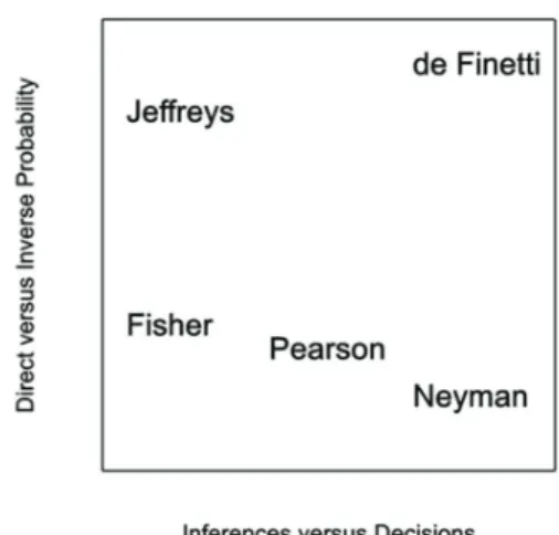
One way of classifying the four systems is in terms of two dimensions each rep-resenting two choices. The first is a choice of making inferences or making de-cisions and the second is whether the stress is on direct or inverse probabili-ties. I prefer the dichotomy direct/inverse to the possible alternative of objec-tive/subjective, since in my opinion Bayesians are happy to use not only sub-jective but also obsub-jective probabilities (after all through their use of Markov Chain Monte Carlo simulations Bayesians are amongst the biggest users of long run relative frequencies) and since many so-called frequentist analyses concern unique events.
Figure 1is a schematic representation of this with the X axis running from inferences on the left to decisions on the right and the Y axis running from direct probability at the bottom to inverse probability at the top.
I have labelled three of the schools by their major proponents. Fisher is, of course,sui generis. Although significance tests are a direct probability de-vice, fiducial probability is more akin to an inverse probability. In the case of
You May Believe You Are a Bayesian But You Are Probably Wrong 57
the Neyman-Pearson school I have decided to represent what I see (agreeing, I think, with Deborah Mayo) as the slightly different positions of its two progeni-tors. Pearson never signed up to the programme of making decisions with power as your guide. He described these as being ways of getting your ideas in gear.
probabil
ing, I thi
never sig
se as be
Figure 1
Because
whateve
in partic
When Fi
say the p
N-P syst
that this
2001, 20
could de
A furthe
ring a pa
itself de
nett 199
than the
the test
statistic
rion of h
another
to be mo
lity. In the ca
nk, with Deb
gned up to t
ing ways of g
. Schematic
e it is useful t
er the system
cular would o
isher’s syste
probability o
tem, where d
s is so since i
002a).They a
ecide whethe
er claimed di
articular test
pends on th
90) Fisher ma
e test statisti
statistic Thu
is back to fr
having a suita
but the only
ore ‘sensitive
ase of the Ne
borah Mayo)
he programm
getting your
illustration o
to have a sin
m, I will use t
object that th
m is compar
of a result as
decisions rat
t is perfectly
are part of th
er a particula
sadvantage o
t to another
e nature of t
akes it clear
ic he does no
us he conside
ont. In his vi
able level of
y basis for pr
e’. On the ot
eyman-Pears
) as the slight
me of makin
ideas in gea
of the major
gle word to
the word
infe
his has no m
ed to the
N-extreme or
her than infe
y possible to
he way in wh
ar hypothesi
of the Fisher
whereas the
the alternativ
that wherea
ot consider t
ers that to m
ew a numbe
significance
referring one
ther hand to
son school I h
tly different
g decisions w
ar.
schools of in
describe the
erence
in con
meaning.
P system ref
more extrem
erences are v
give P-value
hich remote s
s is rejected
rian system i
e N-P system
ve hypothes
as he regards
he alternativ
make the alte
er of differen
. The scienti
e to another
use restricte
have decided
positions of
with power a
nference.
e process of r
nnection wit
ference is oft
me, as being
valued (Good
es a definitio
scientists usi
by them.
s that it seem
can justify t
is. However,
s the null hyp
ve hypothesi
rnative hypo
nt statistics w
st is free to c
would be th
ed tests
beca
d to represen
its two prog
as your guide
reasoning ab
h them all, e
ten made to
a Fisherian d
dman 1992).
n within the
ng different
ms to have n
this in terms
, in a letter to
pothesis as b
is as being m
othesis a just
would satisfy
choose one i
hat in the pas
ause
they fol
nt what I see
genitors. Pea
e. He describ
bout the wor
even though
P-values, th
device alien
. However, I
NP system (
type I error
no basis for p
of power, w
o Chester Bl
being more p
more primitiv
tification for
the Fisheria
in preference
st it had show
llow from a r
e
(agree-arson
bed
the-rld,
Neyman
hat is to
to the
disagree
(Senn
rates
prefer-which
iss
(Ben-primitive
ve than
the test
n
crite-e to
wn itself
restrict-Figure 1: Schematic illustration of the major schools of inference.
Because it is useful to have a single word to describe the process of reasoning about the world, whatever the system, I will use the wordinferencein connection with them all, even though Neyman in particular would object that this has no meaning.
When Fisher’s system is compared to the N-P system reference is often made to P-values, that is to say the probability of a result as extreme or more extreme given that the null hypothesis is true, as being a Fisherian device alien to the N-P system, where decisions rather than inferences are valued (Goodman 1992). However, I disagree that this is so since it is perfectly possible to give P-values a definition within the NP system (Senn 2001; 2002a).They are part of the way in which remote scientists using different type I error rates could decide whether a particular hypothesis is rejected by them.
A further claimed disadvantage of the Fisherian system is that it seems to have no basis for preferring a particular test to another whereas the N-P system can justify this in terms of power, which itself depends on the nature of the alternative hypothesis. However, in a letter to Chester Bliss (Bennett 1990) Fisher makes it clear that whereas he regards the null hypothesis as being more primitive than the test statistic he does not consider the alternative hypothesis as being more primitive than the test statistic. Thus he considers that to make the alternative hypothesis a justification for the test statistic is back to front. In his view a number of different statistics would satisfy the Fisherian criterion of having a suitable level of significance. The scientist is free to choose one in preference to another but the only basis for preferring one to another would be
that in the past it had shown itself to be more ‘sensitive’. On the other hand to use restricted testsbecausethey follow from a restricted set of alternative hypotheses, would be to claim to know more about what must apply if the null hypothesis is false than could ever reasonably be the case.
If any one of the four systems had a claim to our attention then I find de Finetti’s subjective Bayes theory extremely beautiful and seductive (even though I must confess to also having some perhaps irrational dislike of it). The only problem with it is that it seems impossible to apply. I will explain why I think so in due course. I will then provide some examples to try and convince the reader that it is not so easy to apply. In doing so I am well aware that examples are not arguments.
Before I do so, however, I want to make one point clear. I am not arguing that the subjective Bayesian approach is not a good one to use. I am claiming in-stead that the argument is false that because some ideal form of this approach to reasoning seems excellent in theory it therefore follows that in practice us-ing this and only this approach to reasonus-ing is the right thus-ing to do. A very standard form of argument I do object to is the one frequently encountered in many applied Bayesian papers where the first paragraphs lauds the Bayesian approach on various grounds, in particular its ability to synthesise all sources of information, and in the rest of the paper the authors assume that because they have used the Bayesian machinery of prior distributions and Bayes theorem they have therefore done a good analysis. It is this sort of author who believes that he or she is Bayesian but in practice is wrong.
3. Reasons for Hesitation
The first of these is temporal coherence. De Finetti was adamant that it is not the world’s time, in a sense of the march of events (or the history of ‘one damn thing after another’), that governs rational decision making but the mind’s time, that is to say the order in which thoughts occur or evidence arises. However, I do think that he believed there was no going back. You struck out the sequences of thought-events that had not occurred in your mind and renormalized. The discipline involved is so stringent that most Bayesians seem to agree that it is intolerable and there have been various attempts to show that Bayesian infer-ence really doesn’t mean this. I am unconvinced. I think that de Finetti’s theory reallydoesmean this and the consequence is that the phrase ‘back to the draw-ing board’ is not allowed. Attempts to explain away the requirement of temporal coherence always seem to require an appeal to a deeper order of things—a level at which inference really takes place that absolves one of the necessity of doing it properly at the level of Bayesian calculation. This is problematic, because it means that the informal has to come to the rescue of the formal. We concede that the precise Bayesians calculations do not necessarily deliver the right an-swer but this failure of the super-ego does not matter because the id is happily producing a true Bayesian solution.
Note that in making this criticism, I am not criticising informal inference. Indeed, I think it is inescapable. I am criticising claims to have found the perfect system of inference as some form of higher logic because the claim looks rather foolish if the only thing that can rescue it from producing silly results is the operation of the subconscious. Nor am I criticising subjective Bayesianism as a practical tool of inference. As mentioned above, I am criticising the claim that it is the only system of inference and in particular I am criticising the claim that
becauseit is perfect in theory it must be the right thing to use in practice. A related problem is that of Bayesian conversion. Suppose that you are not currently a Bayesian. What does this mean? It means that you currently own up to a series of probability statements that do not form a coherent set. How do you become Bayesian? This can only happen by eliminating (or replacing or modifying) some of the probability statements until you do have a coherent set. However, this is tantamount to saying that probability statements can be dis-owned and if they can be disdis-owned once, it is difficult to see why they cannot be disowned repeatedly but this would seem to be a recipe for allowing individ-uals to pick and choose when to be Bayesian. I sometimes put it like this: the Bayesian theory is a theory of how to remain perfect but it does not explain how to become good.
I think that this is a much more serious problem than many Bayesians sup-pose. It is not just a theoretical problem. I sometimes describe a Bayesian as one who has a reverential awe for all opinions except those of a frequentist statis-tician. It is hard to see what exactly a Bayesian statistician is doing when in-teracting with a client. There is an initial period in which the subjective beliefs of the client are established. These prior probabilities are taken to be valuable enough to be incorporated in subsequent calculation. However, in subsequent steps the client is not trusted to reason. The reasoning is carried out by the statistician. As an exercise inmathematics it is not superior to showing the client the data, eliciting a posterior distribution and then calculating the prior distribution; as an exercise ininferenceBayesian updating does not appear to have greater claims than ‘downdating’ and indeed sometimes this point is made by Bayesians when discussing what their theory implies.
Also related is the date of information problem. It is necessary, to an extent that is often overlooked, to establish exactly what the basis is for any particular prior distributions being established. This, as indeed are all the difficulties, is related to the first one of temporal coherence. It is important to make sure that one knows exactly what was known when. I am often asked by my clients in the pharmaceutical industry whether they should do a Bayesian analysis. I reply that they should when they wish to make a decision but reporting a Bayesian analysis is not a very useful thing to do. Faced with a series of Bayesian analyses one needs to be able to subtract the prior information first in case it or some element of it is common. It is an important irony that a Bayesian statistician wishing to do a Bayesian analysis will (usually) find it easier to do so if presented with a series of frequentist summaries rather than a set of Bayesian posterior distributions.
This is related, I think, to Deborah Mayo’s claim that scientists want to have, “a way to check whether they are being misled by beliefs and biases, in scruti-nizing both their own data and that of other researchers” (Mayo 2004, 103). The problem with prior beliefs and likelihoods is that they are (to a degree specified by the model) exchangeable. Thus, if you have a conjugate beta prior distri-bution equivalent to having seen 50 successes and no failures and then see 50 failures, your posterior inference is the same as if your prior said you had seen 25 successes and 25 failures and you then observed a further 25 successes and 25 failures. Of course, in practice, Bayesians will protest that this is simply a naïve use of conjugate prior distributions and in practice one would treat the two cases differently. I have no objection tothispractice, what I am objecting to is claiming to have a perfect theoretical and logically inescapable contract with the past and the future but making frequent appeal toforce majeure.
This does not let frequentists off the hook. Some frequentist habits also only make sense in the context of making a decision and are not, therefore, useful ways of summarising evidence. For example, if there is any point at all to stan-dard frequentist approaches to sequential analysis it is in the sense of having to make a decision for the given trial. As a summary of evidence, I would not want the adjusted analysis (Senn 2008).
Indeed, I see a lot of value in the distinction that Richard Royal makes be-tween three questions one might ask having completed a study: ‘what should I believe?’, ‘what should I do?’ and ‘what is the evidence?’ (Royall 2004). The like-lihood approach seems an attractive one to dealing with the latter, however, as David Cox (2004) has pointed out, it has problems in dealing with nuisance pa-rameters. In theory, the subjective Bayesian approach should be good at this—in practice, as in the examples below, things are not so simple.
4. Examples
Space does not permit me to discuss these in detail; some of them have been discussed elsewhere.
My first concerns an example of Howson and Urbach (1989). They consider 600 rolls of a die in which four of the possible scores are observed 100 times each but there are 77 ones and 123 twos. The Pearson-Fisher chi-square value on five degrees of freedom is 10.58 and so not significant at the 5% level and H&U conclude that the test has got it badly wrong. They do not say, however, what a Bayesian analysis would show and this is a problem because it is not possible to know what is on the table. Any Bayesian who wishes to claim that a Bayesian analysis would produce a conclusion that we all feel is right should proceed to the demonstration. Here, I believe, one would have to distinguish between two extreme cases: 1. the rolling of the die has been agreed and wit-nessed 2. These are some numbers some philosophers have written down in a book; do they report a real die? (There are, of course, many other intermediate cases.) I have produced an analysis of the first case (Senn 2001) but as far as
I am aware they have not. Using a fairly conventional Bayesian analysis I find that the evidence (if case 1 applies) is not overwhelming that the die is not fair. For case 2, I consider that claiming that the chi-square test was suspectbecause
it failed to detect a problem would be like saying the miller’s scales were faulty because they gave the wrong reading when his thumb was on the pan. The fault would lie with the miller not the scales.
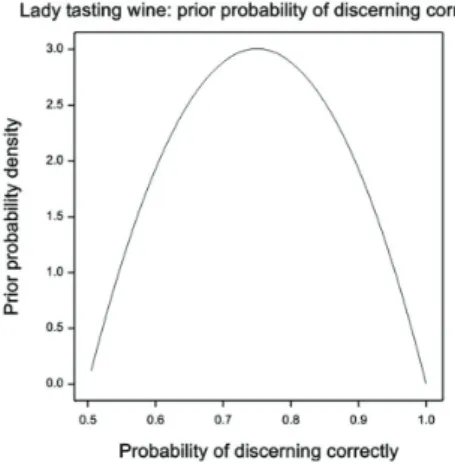
In a second example Denis Lindley (1993) produces a prior distribution for the probability that a lady, holding the ‘Master of Wine’ qualification can discern which of a pair of wine glasses contains claret and which a Californian blend of the same grapes. The prior distribution for her probabilityθ of discerning correctly is given by
f(θ)=48 (1−θ) (θ−1/2) ,θ≥1/2 (13)
This is plotted inFigure 2. I think that it is actually really hard for anybody to come up with a reasonable prior distribution for this example but I am also convinced that nobody not even Lindley would consider that the prior distribu-tion given is reasonable. I would suppose a U shaped distribudistribu-tion of some sort to apply with it being likely that if the lady can distinguish the two she can do so fairly reliably and if not that she will guess. So that far from values near 0.5 and 1 having low probability they have high probability.
Figure 2 scale ag The abo the grou practitio thing tha In a grou Bayesian the anal (Martin first per lowed b 2002b). treatme effect. T model (e one who Various the lead Howeve measure 1008 ho time inte quentist being m distribut In a pap Bayesian
. Plot of Lind ainst probab ve two exam unds that the oners and the
at De Finetti und breaking n approache
ysis of a so-c and Brownin iod followed y treatment This is the re ent period. If The amount o
even if only t ose values ca approaches ding Bayesian er, what nobo
ed 4-8 hours ours. Thus the
erval that is t statistician ore Bayesian tions or even er published n approache
dley’s prior fo bility of disce mples concer ey are not m ese will illust would really g paper publ
s to problem called AB/BA ng 1985). Pat d by treatme
A. The key p esidual effec this happen of carry-over to have it ex an affect infe
to modelling n statistician ody consider after the las e residual ef at least 125 who chose t n in the De F n Bayes facto d in Statistics s to the estim
or the lady ta erning correc rned Bayesia eant to be ta trate that it i y regard as s ished in App ms that arise A cross-over t
tients were r nt with B in a problem in th ct of a treatm s then one is r is usually o
plicitly set to erence.
g the effect o David Spieg red was the a st dose of tre ffect of the p
times as lon to set such a inetti sense ors. s in Medicine
mation of th
asting wine. ctly.
n theoreticia aken serious is possible to such. plied Statistic
in the pharm trial of two d randomised a second pe he analysis o ment given in s in danger o f no great in o zero) and i
of carry-over gelhalter as w actual detail eatment but previous trea ng as the dire carry-over t then one wh
e in 2005 Lam e so-called r
Probability d
ans and perh sly. However o claim to be
cs in 1985 Ra maceutical in doses of a be to one of tw riod or treat of cross-over n an earlier t of making a b
terest in itse s thus an exa
r were consid well as others s of the trial the period o atment (the c ect effect of t to zero (that ho used conv
mbert et al. c random effec
density is plo
haps one can , my further e Bayesian w
acine et al. (1 ndustry. One eta-blocker in wo sequences ment B in th trials is that reatment in biased estim elf but must f ample of a n
dered by the s in discussio . The treatm of treatment carry-over) is treatment (S is to say igno ventional un
considered th cts variance
otted on the
n excuse thes examples co ithout doing
1986) illustra e of them con
n hypertens s: treatment he first period
t of carry-ove a subsequen ate of the tr form part of uisance para
e authors an on of the pap ment effect w t was six wee s measured a Senn 2000b)
ore it) would informative hirteen diffe in meta-ana vertical se on oncern g any-ated ncerned ion t A in a
d fol-er (Senn nt eatment f the ameter:
d also by per. was
eks or after a . A fre-d be
prior
rent lysis. Figure 2: Plot of Lindley’s prior for the lady tasting wine. Probability density is plotted
on the vertical scale against probability of discerning correctly.
The above two examples concerned Bayesian theoreticians and perhaps one can excuse these on the grounds that they are not meant to be taken seriously. How-ever, my further examples concern practitioners and these will illustrate that it is possible to claim to be Bayesian without doing anything that De Finetti would really regard as such.
In a ground breaking paper published inApplied Statisticsin 1985 Racine et al. (1986) illustrated Bayesian approaches to problems that arise in the
pharma-ceutical industry. One of them concerned the analysis of a so-called AB/BA cross-over trial of two doses of a beta-blocker in hypertension (Martin and Browning 1985). Patients were randomised to one of two sequences: treatment A in a first period followed by treatment with B in a second period or treatment B in the first period followed by treatment A. The key problem in the analysis of cross-over trials is that of carry-cross-over (Senn 2002b). This is the residual effect of a treatment given in an earlier treatment in a subsequent treatment period. If this happens then one is in danger of making a biased estimate of the treatment effect. The amount of carry-over is usually of no great interest in itself but must form part of the model (even if only to have it explicitly set to zero) and is thus an example of a nuisance parameter: one whose values can affect inference.
Various approaches to modelling the effect of carry-over were considered by the authors and also by the leading Bayesian statistician David Spiegelhalter as well as others in discussion of the paper. However, what nobody considered was the actual details of the trial. The treatment effect was measured 4–8 hours after the last dose of treatment but the period of treatment was six weeks or 1008 hours. Thus the residual effect of the previous treatment (the carry-over) is measured after a time interval that is at least 125 times as long as the direct effect of treatment (Senn 2000b). A frequentist statistician who chose to set such a carry-over to zero (that is to say ignore it) would be being more Bayesian in the De Finetti sense then one who used conventional uninformative prior distributions or even Bayes factors.
In a paper published inStatistics in Medicinein 2005 Lambert et al. consid-ered thirteen different Bayesian approaches to the estimation of the so-called random effects variance in meta-analysis. This variance is another example of what statisticians call a nuisance parameter—although of some direct interest, its value determines other inferences that are more important. In this example it is a variance of the ‘true’ treatment effect, which is taken to vary from trial to trial. The more important parameter is the average treatment effect, not least because, given no other information, this would be the best guess of the treat-ment effect in any given trial and hence, it is frequently assumed, for any future patient. (Further discussion as to whether this assumption is reasonable has been given in Senn 2000b.)
The paper begins with a section in which the authors make various intro-ductory statements about Bayesian inference. For example, “In addition to the philosophical advantages of the Bayesian approach, the use of these methods has led to increasingly complex, but realistic, models being fitted” and, “an ad-vantage of the Bayesian approach is that the uncertainty in all parameter esti-mates is taken into account” (Lambert et al. 2005, 2402) but whereas one can neither deny that more complex models are being fitted than had been the case until fairly recently, nor that the sort of investigations presented in this paper are of interest, these claims are clearly misleading in at least two respects.
First, the ‘philosophical’ advantages to which the authors refer must surely be to the subjective Bayesian approach outlined above, yet what the paper con-siders is no such thing. None of the thirteen prior distributions considered can
possibly reflect what the authors believe about the random effect variance. One problem, which seems to be common to all thirteen prior distributions, is that they are determined independently of belief about the treatment effect. This is unreasonable since large variation in the treatment effect is much more likely if the treatment effect is large (Senn 2007b). Second, the degree of uncertainty must be determined by the degree of certainty and certainty has to be a matter of belief so that it is hard to see how prior distributions that do not incorporate what one believes can be adequate for the purpose of reflecting certainty and uncertainty.
Certainly, another Bayesian paper on meta-analysis only a few years later (Higgins et al. 2008) agreed implicitly with this, the authors writing: “We as-sume a priori that if an effect exists then heterogeneity exists, although it may be negligible.” This latter paper by the by is also a fine contribution to practical data-analysis but it is not, despite the claim in the abstract, “We conclude that the Bayesian approach has the advantage of naturally allowing for full uncer-tainty, especially for prediction”, a Bayesian analysis in the De Finetti sense. Consider, for example this statement, “An effective number of degrees of free-dom for such a t-distribution is difficult to determine, since it depends on the extent of the heterogeneity and the sizes of the within-study standard errors as well as the number of studies in the meta-analysis.” (Higgins et al. 2008, 145). This may or may not be a reasonable practical approach but it is certainly not Bayesian.
There are two acid tests. The first is that the method must be capable of providing meta-analytic results when there is only one trial. That is to say the want of data must be made good by subjective probability. The practical problem, of course, is that you cannot estimate the way in which the results vary from trial to trial unless you have at least two trials (in fact, in practice more are needed). But to concede this causes a problem for any committed Bayesian.
The second test is that whereas the arrival of new data will, of course, re-quire you to update your prior distribution to being a posterior distribution, no conceivable possible constellation of results can cause you to wish to change your prior distribution. If it does, you had the wrong prior distribution and this prior distribution would therefore have been wrong even for cases that did not leave you wishing to change it. This mean, for example, that model checking is not allowed.
5. Conclusion, a Defence of Eclecticism
The above examples are not a proof of anything: certainly not that analysis that currently sails under a Bayesian flag of convenience is bad. At least in the more applied cases I illustrated I personally would be interested in the results the authors came up with. But not so interested that I would consider them to be the final word on any problem. Also what I would flatly deny is that analyses that so frankly contradict in many respects what pure Bayesian theory dictates should
be done could use any claim such a theory has to coherence as a justification for the analysis performed.
This leaves us, I maintain, with applied Bayesian analysis as currently prac-ticed as one amongst a number of rough and ready tools that we have for look-ing at data. I think we need many such tools because we need mental conflict as much as mental coherence to spur us to creative thinking. When different systems give different answers it is a sign that we need to dig deeper
References
Barnard, G. A. (1996), “Fragments of a Statistical Autobiography”,Student1, 257–68. Bennett, J. H. (1990),Statistical Inference and Analysis Selected Correspondence of R.
A. Fisher, Oxford: Oxford University Press.
Broad, C. (1918), “On the Relation between Induction and Probability”,Mind27, 389– 404.
Cohen, A. and H. B. Sackrowitz (2003), “Methods of Reducing Loss of Efficiency Due to Discreteness of Distributions”,Stat Methods Med Res12, 23–36.
Corcoran, C., C. Mehta and P. Senchaudhuri (2000), “Power Comparisons for Tests of Trend in Dose-response Studies”,Statistics in Medicine19, 3037–3050.
Cox, D. R. (2004), “Comment on Royall”, in: Taper, M. L. and S.R. Lele (eds.),The Nature of Scientific Evidence, Chicago: University of Chicago Press.
Cox, R. T. (1946), “Probability, Frequency and Reasonable Expectation”,American Jour-nal of Physics14, 1–13.
de Finetti, B. D. (1974),Theory of Probability (Volume 1), Chichester: Wiley. — (1975),Theory of Probability (Volume 2), Chichester: Wiley.
Edwards, A. W. F. (2003), “R. A. Fisher—Twice Professor of Genetics: London and Cam-bridge, or ‘A Fairly Well-known Geneticist’ ”,Journal of the Royal Statistical Society Series D—The Statistician52, 311–318.
Fisher, R. A. (1921), “On the ‘Probable Error’ of a Coefficient of Correletaion Deduced from a Small Sample”,Metron1, 3–32.
— (1930),The Genetical Theory of Natural Selection, Oxford: Oxford University Press. Good, I. J. (1983),Good Thinking: The Foundations of Probability and Its Applications,
Minneapolis: University of Minnesota Press.
Goodman, S. N. (1992), “A Comment on Replication, P-values and Evidence”,Statistics in Medicine11, 875–879.
Grafen, A. (2003), “Fisher the Evolutionary Biologist”,Journal of the Royal Statistical Society Series D—-The Statistician52, 319–329.
Higgins J. P., S. Thompson and D. Spiegelhalter (2008), “A Re-evaluation of Random-effects Meta-analysis”,Journal of the Royal Statistical Society, Series A172, 137– 159.
Howson, C. and P. Urbach (1989),Scientific Reasoning: The Bayesian Approach, La Salle: Open Court.
Ivanova, A. and V. W. Berger (2001), “Drawbacks to Integer Scoring for Ordered Cate-gorical Data”,Biometrics57, 567–570.
Jaynes, E. (2003),Probability Theory: The Logic of Science, Cambridge: Cambridge Uni-versity Press.
Jeffreys, H. (1961),Theory of Probability, third ed., Oxford: Clarendon Press.
Lambert, P. C., A. J. Sutton, P. R. Burton, K. R. Abrams and D. R. Jones (2005), “How Vague is Vague? A Simulation Study of the Impact of the Use of Vague Prior Dis-tributions in MCMC Using WinBUGS”,Statistics in Medicine24, 2401–2428. Lindley, D. V. (1985),Making Decisions, second ed., London: Wiley.
— (1993), “The Analysis of Experimental Data: The Appreciation of Tea and Wine”, Teaching Statististics15, 22–25.
— (2006),Understanding Uncertainty, Hoboken: Wiley.
Martin, A. and R. C. Browning (1985), “Metoprolol in the Aged Hypertensive: A Com-parison of Two Dosage Schedules”,Postgrad Med J61, 225–227.
Mayo D. (1996),Error and the Growth of Experimental Knowledge, Chicago: University of Chicago Press.
— (2004), “An Error-statistical Philosophy of Evidence”, in: Taper, M. L. and S. R. Lele (eds.), An Error-statistical Philosophy of Evidence, Chicago: University of Chicago Press.
Neyman, J. and E. S. Pearson (1928), “On the Use and Interpretation of Certain Test Criteria for Purposes of Statistical Inference: Part I”,Biometrika20a, 175–240. — and — (1933), “On the Problem of the Most Efficient Tests of Statistical Hypotheses”,
Philosophical Transactions of the Royal Society of London Series A—Mathematical Physical and Engineering Sciences231, 289–337.
Pitman, E. J. G. (1965),Some Remarks on Statistical Inference, New York: Springer. Racine A., A. P. Grieve, H. Fluhler and A. F. M. Smith (1986), “Bayesian Methods in
Practice—Experiences in the Pharmaceutical-Industry”,Applied Statistics-Journal of the Royal Statistical Society Series C35, 93–150.
Ramsey, F. (1931),Truth and Probability, ed. by R. B. Braithwaite, New York: Harcourt Brace and Company.
Royall, R. (2004), “The Likelihood Paradigm for Statistical Evidence”, in: Taper, M. L. and S. R. Lele (eds.),The Nature of Scientific Evidence, Chicago: University of Chicago Press.
Savage, J. (1954),The Foundations of Statistics, second ed., New York: Wiley.
Senn, S. J. (1996), “Some Statistical Issues in Project Prioritization in the Pharmaceuti-cal Industry”,Statistics in Medicine15, 2689–2702.
— (1998), “Further Statistical Issues in Project Prioritization in the Pharmaceutical In-dustry”,Drug Information Journal32, 253–259.
— (2000a), “Consensus and Controversy in Pharmaceutical Statistics (with Discussion)”, The Statistician49, 135–176.
— (2000b), “The Many Modes of Meta”,Drug Information Journal34, 535–549. — (2001), “Two Cheers for P-values”,Journal of Epidemiology and Biostatistics6, 193–
— (2002a) “A Comment on Replication, P-values and Evidence”,Statistics in Medicine 21, 2437–2444.
— (2002b),Cross-over Trials in Clinical Research, second ed., Chichester: Wiley. — (2003),Dicing with Death, Cambridge: Cambridge University Press.
— (2007a), “Drawbacks to Noninteger Scoring for Ordered Categorical Data”,Biometrics 63, 296–298.
— (2007b), “Trying to Be Precise about Vagueness”, Statistics in Medicine26, 1417– 1430.
— (2008), “Transposed Conditionals, Shrinkage, and Direct and Indirect Unbiasedness”, Epidemiology19, 652–654; discussion 657–658.
Streitberg, B. and J. Röhmel (1990), “On Tests That Are Uniformly More Powerful Than the Wilcoxon-Mann-Whitney Test”,Biometrics46, 481–484.
Talias, M. A. (2007), “Optimal Decision Indices for R&D Project Evaluation in the Phar-maceutical Industry: Pearson Index versus Gittins Index”,European Journal of Op-erational Research177, 1105–1112.