IJCAI ’05
Learning and Inference over Constrained Output
Vasin Punyakanok
Dan Roth
Wen-tau Yih
Dav Zimak
Department of Computer Science
University of Illinois at Urbana-Champaign
{
punyakan, danr, yih, davzimak
}
@uiuc.edu
Abstract
We study learning structured output in a discrimi-native framework where values of the output vari-ables are estimated by local classifiers. In this framework, complex dependencies among the out-put variables are captured by constraints and dictate which global labels can be inferred. We compare two strategies, learning independent classifiers and
inference based training, by observing their
behav-iors in different conditions. Experiments and theo-retical justification lead to the conclusion that using inference based learning is superior when the lo-cal classifiers are difficult to learn but may require many examples before any discernible difference can be observed.
1
Introduction
Making decisions in real world problems involves assigning values to sets of variables where a complex and expressive structure can influence, or even dictate, what assignments are possible. For example, in the task of identifying named enti-ties in a sentence, prediction is governed by constraints like “entities do not overlap.” Another example exists in scene in-terpretation tasks where predictions must respect constraints that could arise from the nature of the data or task, such as “humans have two arms, two legs, and one head.”
There exist at least three fundamentally different solutions to learning classifiers over structured output. In the first, structure is ignored; local classifiers are learned and used to predict each output component separately. In the sec-ond, learning is decoupled from the task of maintaining struc-tured output. Estimators are used to produce global out-put consistent with the structural constraints only after they are learned for each output variable separately. Discrimina-tive HMM, conditional models [Punyakanok and Roth, 2001; McCallum et al., 2000] and many dynamic programming based schemes used in the context of sequential predictions fall into the this category. The third class of solutions in-corporates dependencies among the variables into the learn-ing process to directly induce estimators that optimize a global performance measure. Traditionally these solutions were generative; however recent developments have pro-duced discriminative models of this type, including
condi-tional random fields [Lafferty et al., 2001], Perceptron-based learning of structured output [Collins, 2002; Carreras and M`arquez, 2003] and Max-Margin Markov networks which allow incorporating Markovian assumptions among output variables [Taskar et al., 2004].
Incorporating constraints during training can lead to solu-tions that directly optimize the true objective function, and hence, should perform better. Nonetheless, most real world applications using this technique do not show significant ad-vantages, if any. Therefore, it is important to discover the tradeoffs of using each of the above schemes.
In this paper, we compare three learning schemes. In the first, classifiers are learned independently (learning only (LO)), in the second, inference is used to maintain struc-tural consistency only after learning (learning plus inference (L+I)), and finally inference is used while learning the pa-rameters of the classifier (inference based training (IBT)). In semantic role labeling (SRL), it was observed [Punyakanok
et al., 2004; Carreras and M`arquez, 2003 ] that when the
lo-cal classification problems are easy to learn, L+I outperforms IBT. However, when using a reduced feature space where the problem was no longer (locally) separable, IBT could over-come the poor local classifications to yield accurate global classifications.
Section 2 provides the formal definition of our problem. For example, in Section 3, we compare the three learning schemes using the online Perceptron algorithm applied in the three settings (see [Collins, 2002] for details). All three set-tings use the same linear representation, and L+I and IBT share the same decision function space. Our conjectures of the relative performance between different schemes are pre-sented in Section 4. Despite the fact that IBT is a more pow-erful technique, in Section 5, we provide an experiment that shows how L+I can outperform IBT when there exist accu-rate local classifiers that do not depend on structure, or when there are too few examples to learn complex structural depen-dencies. This is also theoretically justified in Section 6.
2
Background
Structured output classification problems have many flavors. In this paper, we focus on problems where it is natural both to split the task into many smaller classification tasks and to solve directly as a single task. In Section 5.2, we consider the
semantic role-labeling problem, where the inputX are nat-ural language features and the outputY is the position and type of a semantic-role in the sentence. For this problem, one can either learn a set of local functions such as “is this phrase an argument of ’run’,” or a global classifier to pre-dict all semantic-roles at once. In addition, natural structural constraints dictate, for example, that no two semantic roles for a single verb can overlap. Other structural constraints, as well as linguistic constraints yield a restricted output space in which the classifiers operate.
In general, given an assignment x ∈ Xnx to a
collec-tion of input variables, X = (X1, . . . , Xnx), the struc-tured classification problem involves identifying the “best” assignment y ∈ Yny to a collection of output variables Y = (Y1, . . . , Yny)that are consistent with a defined struc-ture onY. This structure can be thought of as constraining the output space to a smaller spaceC(Yny) ⊆ Yny, where
C: 2Y∗
→2Y∗
constrains the output space to be structurally consistent.
In this paper, a structured output classifier is a function h : Xnx → Yny, that uses a global scoring function,
f : Xnx × Yny → IRto assign scores to each possible
ex-ample/label pair. Given inputx, it is hoped that the correct outputyachieves the highest score among consistent outputs:
ˆ
y=h(x) = argmax
y∈C(Yny)f(x,y
), (1)
wherenxandnydepend on the example at hand. In addition, we view the global scoring function as a composition of a set of local scoring functions{fy(x, t)}y∈Y, wherefy : Xnx×
{1, . . . , ny} → IR. Each function represents the score or confidence that output variableYttakes valuey:
f(x,(y1, . . . , yny)) = ny
t=1
fyt(x, t)
Inference is the task of determining an optimal
assign-ment y given an assignment x. For sequential structure of constraints, polynomial-time algorithms such as Viterbi or CSCL [Punyakanok and Roth, 2001] are typically used for efficient inference. For general structure of constraints, a generic search method (e.g., beam search) may be ap-plied. Recently, integer programming has also been shown to be an effective inference approach in several NLP applica-tions [Roth and Yih, 2004; Punyakanok et al., 2004 ].
In this paper, we consider classifiers with linear
rep-resentation. Linear local classifiers are linear functions, fy(x, t) = αy ·Φy(x, t), where αy ∈ IRdy is a weight
vector and Φy(x, t) ∈ IRdy is a feature vector. Then,
it is easy to show that the global scoring function can be written in the familiar form f(x,y) = α · Φ(x,y), whereΦy(x,y) = ny
t=1Φyt(x, t)I{yt=y} is an
accumula-tion over all output variables of features occurring for class y, α = (α1, . . . ,α|Y|) is concatenation of the αy’s, and Φ(x,y) = (Φ1(x,y), . . . ,Φ|Y|(x,y))is the concatenation of theΦy(x,y)’s. Then, the global classifier is
h(x) = ˆy= argmax
y∈C(Yny)α·Φ(x,y
).
3
Learning
We present several ways to learn the scoring function pa-rameters differing in whether or not the structure-based in-ference process is leveraged during training. Learning con-sists of choosing a functionh : X∗ → Y∗ from some hy-pothesis space,H. Typically, the data is supplied as a set
D = {(x1,y1), . . . ,(xm,ym)} from a distribution PX,Y overX∗× Y∗. While these concepts are very general, we fo-cus on online learning of linear representations using a variant of the Perceptron algorithm (see [Collins, 2002]).
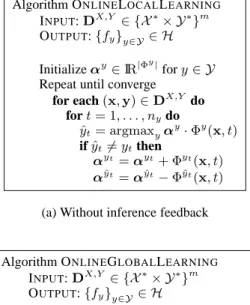
Learning Local Classifiers: Learning stand-alone local classifiers is perhaps the most straightforward setting. No knowledge of the inference procedure is used. Rather, for each example(x,y) ∈ D, the learning algorithm must en-sure thatfyt(x, t) > fy(x, t)for allt = 1, . . . , ny and all y =yt. In Figure 3(a), an online Perceptron-style algorithm is presented where no global constraints are used. See [Har-Peled et al., 2003] for details and Section 5 for experiments.
Learning Global Classifiers: We seek to train classifiers
so they will produce the correct global classification. To this end, the key difference from learning locally is that feed-back from the inference process determines which classifiers to modify so that together, the classifiers and the inference procedure yield the desired result. As in [Collins, 2002; Carreras and M`arquez, 2003], we train according to a global criterion. The algorithm presented here is an online proce-dure, where at each step a subset of the classifiers are up-dated according to inference feedback. See Figure 3(b) for details of a Perceptron-like algorithm for learning with infer-ence feedback.
Note that in practice it is common for problems to be mod-eled in such a way that local classifiers are dependent on part of the output as part of their input. This sort of interaction can be incorporated directly to the algorithm for learning a global classifier as long as an appropriate inference process is used. In addition, to provide a fair comparison between LO, L+I, and IBP in this setting one must take care to ensure that the learning algorithms are appropriate for this task. In order to remain focused on the problem of training with and without inference feedback, the experiments and analysis presented concern only the local classifiers without interaction.
4
Conjectures
In this section, we investigate the relative performance of classifier systems learned with and without inference feed-back. There are many competing factors. Initially, if the lo-cal classification problems are “easy”, then it is likely that learning local classifiers only (LO) can yield the most accu-rate classifiers. However, an accuaccu-rate model of the structural constraints could additionally increase performance (learning plus inference (L+I)). As the local problems become more difficult to learn, an accurate model of the structure becomes more important, and can, perhaps, overcome sub-optimal lo-cal classifiers. Despite the existence of a global solution, as the local classification problems become increasingly diffi-cult, it is unlikely that structure based inference can fix poor classifiers learned locally. In this case, only training with in-ference feedback (IBT) can be expected to perform well.
Algorithm ONLINELOCALLEARNING
INPUT:DX,Y ∈ {X∗× Y∗}m OUTPUT:{fy}y∈Y∈ H Initializeαy∈IR|Φy|fory∈ Y
Repeat until converge for each(x,y)∈DX,Y do
fort= 1, . . . , nydo ˆ
yt= argmaxyαy·Φy(x, t)
ifyˆt=ytthen
αyt =αyt+ Φyt(x, t)
αˆyt =αyˆt−Φyˆt(x, t)
(a) Without inference feedback
Algorithm ONLINEGLOBALLEARNING
INPUT:DX,Y ∈ {X∗× Y∗}m OUTPUT:{fy}y∈Y∈ H
Initializeα∈IR|Φ| Repeat until converge
for each(x,y)∈DX,Y do ˆ
y= argmaxy∈C(Yny)α·Φ(x,y)
ifyˆ=ythen
α=α+ Φ(x,y)−Φ(x,yˆ)
(b) With inference feedback
Figure 1: Algorithms for learning without and with infer-ence feedback. The key differinfer-ence lies in the inferinfer-ence step (i.e. argmax). Inference while learning locally is trivial and the prediction is made simply by considering each la-bel locally. Learning globally uses a global inference (i.e. argmaxy∈C(Yny)) to predict global labels.
As a first attempt to formalize the difficulty of classifica-tion tasks, we define separability and learnability. A classi-fier,f ∈ H, globally separates a data setDiff for all exam-ples(x,y) ∈ D,f(x,y) > f(x,y)for ally ∈ Yny \y
and locally separates D iff for all examples (x,y) ∈ D, fyt(x, t)> fy(x, t)for ally∈ Y \yt, and ally∈ Yny \y.
A learning algorithmAis a function from data sets to aH. We say thatD is globally (locally) learnable byAif there exists anf ∈ Hsuch thatf globally (locally) separatesD.
The following simple relationships exist between local and global learning: 1. local separability implies global separa-bility, but the inverse is not true;2.local separability implies local and global learnability; 3. global separability implies global learnability, but not local learnability. As a result, it is clear that if there exist learning algorithms to learn global sep-arations, then given enough examples, IBT will outperform L+I. However, learning examples are often limited either be-cause they are expensive to label or bebe-cause some learning algorithms simply do not scale well to many examples. With a fixed number of examples, L+I can outperform IBT.
Claim 4.1 With a fixed number of examples:
1. If the local classification tasks are separable, then L+I outperforms IBT.
2. If the task is globally separable, but not locally sepa-rable then IBT outperforms L+I only with sufficient ex-amples. This number correlates with the degree of the separability of the local classifiers.
5
Experiments
We present experiments to show how the relative performance of learning plus inference (L+I) compares to inference based training (IBT) when the quality of the local classifiers and amount of training data varies.
5.1
Synthetic Data
In our experiment, each examplexis a set ofcpoints ind -dimensional real space, wherex= (x1,x2, . . . ,xc)∈IRd× . . .×IRdand its label is a sequence of binary variable,y= (y1, . . . , yc)∈ {0,1}c, labeled according to:
y=h(x) = argmax
y∈C(Yc)
i
yifi(xi)−(1−yi)fi(xi), whereC(Yc)is a subset of{0,1}c imposing a random con-straint1ony, andfi(xi) =wixi+θi. Eachficorresponds to a local classifieryi=gi(xi) =Ifi(xi)>0. Clearly, the dataset generated from this hypothesis is globally linearly separable. To vary the difficulty of local classification, we generate ex-amples with various degree of linear separability of the lo-cal classifiers by controlling the fractionκof the data where h(x) =g(x) = (g1(x1), . . . , gc(xc))—examples whose la-bels, if generated by local classifiers independently, violate the constraints (i.e.g(x)∈ C/ (Yc)).
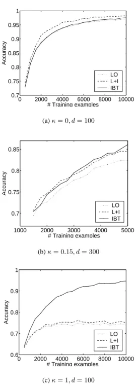
Figure 2 compares the performance of different learning strategies relative to the number of training examples used. In all experiments,c= 5, the true hypothesis is picked at ran-dom, andC(Yc)is a random subset with half of the size of
Yc. Training is halted when a cycle complete with no errors, or 100 cycles is reached. The performance is averaged over 10 trials. Figure 2(a) shows the locally linearly separable case where L+I outperforms IBT. Figure 2(c) shows results for the case with the most difficult local classification tasks(κ = 1) where IBT outperforms L+I. Figure 2(b) shows the case where data is not totally locally linearly separable(κ= 0.1). In this case, L+I outperforms IBT when the number of train-ing examples is small. In all cases, inference helps.
5.2
Real-World Data
In this section, we present experiments on two real-world problems from natural language processing – semantic role labeling and noun phrase identification.
Semantic-Role Labeling
Semantic role labeling (SRL) is believed to be an important
task toward natural language understanding, and has imme-diate applications in tasks such Information Extraction and
1
Among the total2cpossible output labels,C(·)fixes a random fraction as legitimate global labels.
0 2000 4000 6000 8000 10000 0.7
0.75 0.8 0.85 0.9 0.95 1
# Training examples
Accuracy
LO L+I IBT
(a)κ= 0, d= 100
1000 2000 3000 4000 5000 0.7
0.75 0.8 0.85
# Training examples
Accuracy
LO L+I IBT
(b)κ= 0.15, d= 300
0 2000 4000 6000 8000 10000 0.6
0.7 0.8 0.9 1
# Training examples
Accuracy
LO L+I IBT
(c)κ= 1, d= 100
Figure 2: Comparison of different learning strategies in various degrees of difficulties of the local classifiers.κ= 0implies locally linearly separability. Higherκindicates harder local classification.
Question Answering. The goal is to identify, for each verb in the sentence, all the constituents which fill a semantic role, and determine their argument types, such as Agent, Patient,
Instrument, as well as adjuncts such as Locative, Temporal, Manner, etc. For example, given a sentence “ I left my pearls
to my daughter-in-law in my will”, the goal is to identify dif-ferent arguments of the verb left which yields the output:
[A0I] [Vleft] [A1my pearls] [A2to my daughter-in-law]
103 104 105 106 107 50
55 60 65 70 75 80
Separability (# Features)
F1
LO L+I IBT
103 104 105 106 107 50
55 60 65 70 75 80
Separability (# Features)
F1
LO L+I IBT
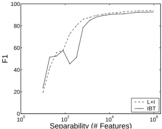
Figure 3:Results on the semantic-role labeling (SRL) problem. As the number of features increases, the difficulty of the local classifi-cation problem becomes easier, and the independently learned clas-sifiers (LO) perform well, especially when inference is used after learning (L+I). Using inference during training (IBT) can aid perfor-mance when the learning problem is more difficult (few features).
[AM-LOCin my will].
Here A0 represents leaver, A1 represents thing left, A2 rep-resents benefactor, AM-LOC is an adjunct indicating the lo-cation of the action, and V determines the verb.
We model the problem using classifiers that map con-stituent candidates to one of 45 different types, such as fAO and fA1 [Kingsbury and Palmer, 2002; Carreras and M`arquez, 2003]. However, local multiclass decisions are in-sufficient. Structural constraints are necessary to ensure, for example, that no arguments can overlap or embed each other. In order to include both structural and linguistic constraints, we use a general inference procedure based on integer linear programming [Punyakanok et al., 2004]. We use data pro-vided in the CoNLL-2004 shared task [Carreras and M`arquez, 2003], but we restrict our focus to sentences that have greater than five arguments. In addition, to simplify the problem, we assume the boundaries of the constituents are given – the task is mainly to assign the argument types.
The experiments clearly show that IBT outperforms lo-cally learned LO and L+I when the local classifiers are in-separable and difficult to learn. The difficulty of local learn-ing was controlled by varylearn-ing the number of input features. With more features, the linear classifier are more expressive and can learn effectively and L+I outperforms IBT. With less features the problem becomes more difficult and IBT outper-forms L+I. See Figure 3.
Noun Phrase Labeling
Noun phrase identification involves the identification of phrases or of words that participate in a syntactic relation-ship. Specifically, we use the standard base Noun Phrases (NP) data set [Ramshaw and Marcus, 1995] taken from the Wall Street Journal corpus in the Penn Treebank [Marcus et
al., 1993].
100 102 104 106 0
20 40 60 80 100
Separability (# Features)
F1
L+I IBT
Figure 4: Results on the noun phrase (NP) identification prob-lem.
detects the beginning,f[, and a second that detects the end, f]of a phrase. The outcome of these classifiers are then com-bined in a way that satisfies structural constraints constraints (e.g. non-overlapping), using an efficient constraint satisfac-tion mechanism that makes use of the confidence in the clas-sifiers’ outcomes [Punyakanok and Roth, 2001].
In this case, L+I trains each classifier independently, and only during evaluation, the inference is used. On the other hand, IBT incorporates the inference into the training. For each sentence, each word position is processed by the clas-sifiers, and their outcomes are used by the inference process to infer the final prediction. The classifiers are then updated based on the final prediction not on their own prediction be-fore the inference.
As in the previous experiment, Figure 4 shows perfor-mance of two systems varied by the number of features. Un-like the previous experiment, the number of features in each experiment was determined by the frequency of occurrence. Less frequent features are pruned to make the task more diffi-cult. The results are similar to the SRL task in that only when the problem becomes difficult IBT outperforms L+I.
6
Bound Prediction
In this section, we use standard VC-style generalization bounds from learning theory to gain intuition into when learn-ing locally (LO and L+I) may outperform learnlearn-ing globally (IBT) by comparing the expressivity and complexity of each hypothesis space. When learning globally, it is possible to learn concepts that may be difficult to learn locally, since the global constraints are not available to the local algorithms. On the other hand, while the global hypothesis space is more expressive, it has a substantially larger representation. here we develop two bounds—both for linear classifiers on a re-stricted problem. The first upper bounds the generalization error for learning locally by assuming various degrees of sep-arability. The second provides an improved generalization bound for globally learned classifiers by assuming separabil-ity in the more expressive global hypothesis space.
We begin by defining the growth function to measure the effective size of the hypothesis space.
Definition 6.1 (Growth Function) For a given hypothesis
classHconsisting of functionsh:X → Y, the growth
func-tion,NH(m), counts the maximum number of ways to label any data set of sizem:
NH(m) = sup
x1,...,xm∈Xm
|{(h(x1), . . . , h(xm))|h∈ H}| The well-known VC-style generalization bound expresses expected error,, of the best hypothesis,hopton unseen data. In the following theorem adapted from [Anthony and Bartlett, 1999][Theorem 4.2], we directly write the growth function into the bound,
Theorem 6.2 Suppose thatHis a set of functions from a set
X to a setY with growth functionNH(m). Lethopt ∈ H
be the hypothesis that minimizes sample error on a sample of sizemdrawn from an unknown, but fixed probability distri-bution. Then, with probability1−δ
≤opt+
32(log(NH(2m)) + log(4/δ))
m . (2)
For simplicity, we first describe the setting in which a sep-arate function is learned for each of a fixed number, c, of output variables (as in Section 5.1). Here, each example has ccomponents in inputx= (x1, . . . ,xc)∈ IRd×. . .×IRd and outputy= (y1, . . . , yc)∈ {0,1}c.
Given a datasetD, the aim is to learn a set of linear scor-ing functions fi(xi) = wixi, where wi ∈ IRd for each i = 1, . . . , c. For LO and L+I, the setting is simple: find a set of weight vectors that, for each component, satisfy yiwixi >0for all examples(x,y)∈ D. For IBT, we find a set of classifiers such thatiyiwixi >iyiwixi for all y =y(and that satisfy the constraints,y ∈ C(Yc)).
As previously noted, when learning local classifiers inde-pendently (LO and L+I), one can only guarantee convergence when each local problem is separable – however, it is often the case that global constraints render these problems insepa-rable. Therefore, there is a lower bound,opt, on the optimal error achievable. Since each component is a separate learning problem, the generalization error is thus
Corollary 6.3 WhenHis the set of separating hyperplanes inIRd,
≤opt+
32(dlog((em/d)) + log(4/δ))
m . (3)
Proof sketch: We show that NH(m) ≤ (em/d)d when H is the class of threshold linear functions in d dimensions.
NH(m) is precisely the maximum number of continuous
regions an arrangement of m halfspaces in IRd, which is 2d
i=1
m−1
i
≤ 2(e(m−1)/d)d. Form > 1, the result holds. See [Anthony and Bartlett, 1999][Theorem 3.1] for details.
On the other hand, when learning collectively with IBT, examples consist of the full vectorx ∈ IRcd. In this set-ting, convergence is guaranteed (if, of course, such a function
0 2 4 6 8 10 x 105 0
0.1 0.2 0.3 0.4 0.5 0.6 0.7 0.8 0.9 1
Number of Examples
Accuracy
IBT e
opt = 0 e
opt = 0.1 e
opt = 0.2
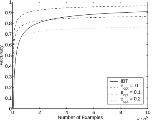
Figure 5:The VC-style generalization bounds predict that IBT will eventually outperform LO if the local classifiers are unable to find consistent classification (opt >0.0, accuracy <1). However, if
the local classifiers are learnable (opt = 0.0, accuracy = 1), LO will perform well.
exists). Thus, the optimal error when training with IBT is opt = 0. However, the output of the global classification is now the entire output vector. Therefore, the growth function must account for exponentially many outputs.
Corollary 6.4 WhenHis the set of decision functions over
{0,1}c, defined byargmaxy∈C({0,1}c)ci=1yiwixi, where w= (w1, . . . ,wc)∈IRcd,
≤
32(cdlog(em/cd) +c2d+ log(4/δ))
m . (4)
Proof sketch: In this setting, we must count the effective
hypothesis space – which is the effective number of differ-ent classifiers in weight space,IRcd. As before, this is done by constructing an arrangement of halfspaces in the weight space. Specifically, each halfspace is defined by a single ((x,y),y)pair that defines the region whereiyiwixi >
iyiwixi. Because there are potentiallyC(2c) ≤ 2c out-put labels and the weight space iscd-dimensional, the growth function is the size of the arrangement ofc2c halfspaces in
IRcd. ThereforeNH(m)≤(em2c/cd)cd.
Figure 5 shows a comparison between these two bounds, where the generalization bound curves on accuracy are shown for IBT (Corollary 6.4) and for LO and L+I (Corollary 6.3) withopt ∈ {0.0,0.1,0.2}. One can see that when separa-ble, the accuracy=1 curve (opt = 0.0) in the figure outper-forms IBT. However, when the problems are locally insepara-ble, IBT will eventually converge, whereas LO and L+I will not – these results match the synthetic experiment results in Figure 2. Notice the relationship betweenκandopt. When κ= 0, both the local and global problems are separable and opt = 0Asκincreases, the global problem remains separa-ble and the local prosepara-blems are inseparasepara-ble (opt>0).
7
Conclusion
We studied the tradeoffs between three common learning schemes for structured outputs, i.e. learning without the knowledge about structure (LO), using inference only after learning (L+I), and learning with inference feedback (IBT).
We provided experiments on both real-world and synthetic data as well as a theoretical justification that support our main clams. – first, when the local classification is linearly sepa-rable, L+I outperforms IBT, and second, as the local prob-lems become more difficult and are no longer linearly sepa-rable, IBT outperforms L+I, but only with sufficient number of training examples. In the future, we will seek a similar comparison for the more general setting where nontrivial in-teraction between local classifiers is allowed, and thus, local separability does not imply global separability.
8
Acknowledgments
We grateful Dash Optimization for the free academic use of Xpress-MP. This research is supported by the Advanced Research and De-velopment Activity (ARDA)’s Advanced Question Answering for Intelligence (AQUAINT) Program, a DOI grant under the Reflex program, NSF grants ITR-0085836, ITR-0085980 and IIS-9984168, and an ONR MURI Award.
References
[Anthony and Bartlett, 1999] M. Anthony and P. Bartlett. Neural
Network Learning: Theoretical Foundations. Cambridge
Uni-versity Press, 1999.
[Carreras and M`arquez, 2003] X. Carreras and Llu´ıs M`arquez. On-line learning via global feedback for phrase recognition. In
Ad-vances in Neural Information Processing Systems 15, 2003.
[Collins, 2002] M. Collins. Discriminative training methods for hidden Markov models: Theory and experiments with perceptron algorithms. In Proceedings of EMNLP, 2002.
[Har-Peled et al., 2003] S. Har-Peled, D. Roth, and D. Zimak. Con-straint classification: A new approach to multiclass classification and ranking. In Advances in Neural Information Processing
Sys-tems 15, 2003.
[Kingsbury and Palmer, 2002] P. Kingsbury and M. Palmer. From Treebank to PropBank. In Proceedings of LREC, 2002.
[Lafferty et al., 2001] J. Lafferty, A. McCallum, and F. Pereira. Conditional random fields: Probabilistic models for segmenting and labeling sequence data. In Proc. ICML-01, pages 282–289, 2001.
[Marcus et al., 1993] M. P. Marcus, B. Santorini, and M. Marcinkiewicz. Building a large annotated corpus of English: The Penn Treebank. Computational Linguistics,
19(2):313–330, June 1993.
[McCallum et al., 2000] A. McCallum, D. Freitag, and F. Pereira. Maximum entropy Markov models for information extraction and segmentation. In Proceedings of ICML-00, Stanford, CA, 2000.
[Punyakanok and Roth, 2001] V. Punyakanok and D. Roth. The use of classifiers in sequential inference. In Advances in Neural
In-formation Processing Systems 13, 2001.
[Punyakanok et al., 2004] V. Punyakanok, D. Roth, W. Yih, and D. Zimak. Semantic role labeling via integer linear programming inference. In Proceedings of COLING-04, 2004.
[Ramshaw and Marcus, 1995] L. A. Ramshaw and M. P. Marcus. Text chunking using transformation-based learning. In
Proceed-ings of the Third Annual Workshop on Very Large Corpora, 1995.
[Roth and Yih, 2004] D. Roth and W. Yih. A linear programming formulation for global inference in natural language tasks. In
Proceedings of CoNLL-2004, pages 1–8, 2004.
[Taskar et al., 2004] B. Taskar, C. Guestrin, and D. Koller. Max-margin markov networks. In Advances in Neural Information
![AENG100Z Introduction to Analytical Writing [Open to Freshman and Sophomores Only]](data:image/gif;base64,R0lGODlhAQABAIAAAP///wAAACH5BAEAAAAALAAAAAABAAEAAAICRAEAOw==)