A BRIEF INTRODUCTION TO STATA
WITH 50+ BASIC COMMANDS
Tobias Pfaff
*Institute for Economic Education, University of Münster
Version: October 2009
Table of contents
1. Why Stata? ... 1
2. How to work with the software ... 3
2.1. User-interface ... 3
Results window ... 3
Command window ... 3
Variables window ... 3
Review window ... 4
Buttons ... 4
Menu ... 4
2.2. Do-files ... 4
2.3. Limits of the software ... 5
3. General commands ... 6
cd ... 6
help ... 7
update ... 6
findit ... 7
set memory ... 7
display ... 8
4. Data input and saving ... 8
use ... 8
insheet ... 8
edit ... 9
compress ... 9
save ... 9
5. Data management ... 9
5.1. General command syntax ... 9
by ... 10
in ... 12
5.2. Commenting ... 12
5.3. Data description... 17
describe ... 17
codebook ... 17
sort ... 18
order ... 18
browse ... 18
list ... 19
assert ... 19
summarize ... 19
tabulate ... 19
inspect ... 20
5.4. Data manipulation ... 13
generate ... 13
egen ... 14
replace ... 14
recode ... 14
drop ... 15
keep ... 15
destring ... 15
5.5. Data formatting ... 16
rename ... 16
recast ... 16
format ... 17
label ... 17
5.6. Data merging ... 20
append ... 20
merge ... 20
6. Further issues ... 22
6.1. Log files ... 22
6.3. Probability distribution and density functions ... 22
6.4. Random number generation ... 23
7. Shortcuts (that make “life” easier) ... 23
8. Some sample do-files ... 23
8.1. Example for importing data ... 23
8.2. Example for preparing data ... 24
8.3. Example for analyzing data ... 25
8.4. Example for do-file that runs the entire project ... 26
9. What is not captured in this introduction... 26
10. Where to find help ... 27
10.1. In-built help and printed manuals ... 27
10.2. Online resources ... 27
1. Why Stata?
Choosing a statistical software package in a company or research institution is often a strategic decision. The decision entails the investment of time and money, and you should think about the future development and compatibility of the software. Often, it is also influential what type of software your peer group is using, since this is usually the main source for getting support and exchanging experience.
The main software bundles for statistical computing are R (www.r-project.org), SAS (www.sas.com), SPSS (www.spss.com), and Stata (www.stata.com). However, there are many more packages in the market, some of them specialized for specific statistical problems. A general overview as well as a simple comparison of statistical packages is given on Wikipedia (http://en.wikipedia.org/wiki/Comparison_of_statistical_packages). Statistical software can either be used by command line or by point-and-click menus, or both. The command line usage has the invaluable advantage that all steps of the analysis, and thus all results, are easily replicable. In contrast, menu usage might make it very difficult to replicate results, especially in larger projects. However, it might be more difficult in the beginning to learn a new command structure, especially for those users who have never worked with programming languages. Nonetheless, initial ease of use should be weighed against long-term payoffs before choosing the software.
Each software package can be distinguished by several factors. Some of the major factors
are depicted (very) simplistically in the following table:1
R SAS SPSS Stata
Price ++
(free)
- -- +
Command structure + + -- ++
Support + - -- ++
Ease of teaching + -- - ++
1 This and the rest of this section has partly been adopted from: Acock, A. (2005), SAS, Stata, SPSS: A Comparison, Journal of Marriage & Family, 67 (4), pp. 1093–1095. And from: Mitchell, M. (2007), Strategically using General Purpose Statistics Packages: A Look at Stata, SAS and SPSS, Report No. 1, Technical Report Series, UCLA Academic Technology Services.
R:
R is a free software package which is designed for use with command line only. While being a language is one of R's greatest strengths, it can make it harder to learn for those without programming experience. However, once learnt, you are no longer subject to price increases. The developer’s community ensures to constantly provide add-ons and also ensures that the software will continue to exist. R is extremely versatile in graphics, and generally good for people who really want to find out “what their data have to say”. SAS:
SAS is the second most costly package. It can be used with, both, command line and graphical user interface (GUI). SAS is particularly strong on data management (especially with large files), and good for cutting edge research. It covers many graphical and statistical tasks. The main focus is on business customers now.
SPSS:
SPSS is the first choice for the occasional user. However, it is the most expensive of the four. SPSS is clearly designed for point-and-click usage on the GUI. A command structure exists, but it is not well defined and sometimes inconsistent. SPSS is good for basic data management and basic statistical analysis, but rather weak in graphics. In the future, SPSS might be the weakest of the four packages with regard to the scope of statistical procedures it offers due to its main focus on business customers.
Stata:
Stata is designed for the usage by command line, but it also offers a GUI that allows for working with menus. The simple and consistent command structure makes it rather easy to learn. It is the cheapest of the packages that entail costs, and it offers additional reductions for the educational sector. Stata is relatively weak on ANOVA, but extraordinary on regression analysis and complex survey designs. Stata is completely focused on scholars. In the future, Stata may have the strongest collection of advanced statistical procedures.
2. How to work with the software
2.1. User-interface
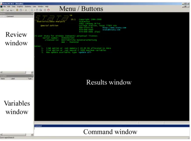
The Stata user-interface consists of the following elements:
Figure 1: Screenshot of Stata user-interface
Results window
All outputs appear in this window. Only graphics will appear in a separate window.
Command window
This is the command line where commands are entered for execution.
Variables window
All variables in the currently open dataset will appear here. By clicking on a variable its name can be transferred to the command window.
Review window
Previously used commands are listed here and can be transferred to the command window by clicking on them.
Buttons
The most important button functions are the following:
• Open (use): Opens a new data file.
• Save: Saves the current data file.
• Print results: Prints the content of the results window.
• New Viewer: Opens a new viewer window, e.g. to open log-files.
• New Do-file Editor: Opens a new instance of the do-file editor (same as doedit).
• Data Editor: Opens the data editor window (same as edit).
• Data Browser: Opens the data browser (same as browse).
• Break: Allows to cancel currently running calculations.
Menu
Almost all commands can be called from the menu. However, we do not recommend to learn Stata using the menu commands since the command line will give the user much better control and allows for a much faster and more exact working process.
2.2. Do-files
The crucial advantage of using the command line instead of point-and-click menus is that it allows for the replication of results. However, all typed commands are lost once Stata is closed (unless you manually start a command log). This can be avoided by using so-called “do-files” where Stata commands are saved as a script in a simple text file with the ending “.do”. When the do-file is run using the do-file editor all commands are executed subsequently. If all steps of a project have been documented in one or more do-files, all analyses and results can be reproduced and the whole process can be retraced by third party people.
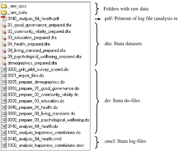
However, saving all commands for a (bigger) project in a single do-file should be avoided. Rather, it is recommended to split up commands in several do-files named according to the respective step in the process (e.g., data import, data management, data
analysis). The following shows an example of how such a do-file cascade could look like in a project folder (leading numbers indicate the chronology of the working process):
Figure 2: Example of a project folder
2.3. Limits of the software
At certain points during your work with Stata you might encounter its limits. In order not to be surprised by sudden error messages, it is useful to be aware of the limits, which
depend on the package version of Stata (the command help limits shows the limits):
Folders with raw data
.pdf: Printout of log file (analysis results)
.dta: Stata datasets
.do: Stata do-files
Stata package: Small Intercooled SE
See www.stata.com/order for licence fees of the packages.
# of observations 1,200 unlimited unlimited
# of variables 99 2,047 32,767
# of characters in a command 8,697 67,800 1,081,527
# of options for a command 70 70 70
Length of a string variable 244 244 244
Length of a variable name 32 32 32
3. General commands
update
Stata offers a convenient update function over the internet. The update status of the currently installed Stata version can be compared with the one on the Stata website using
update query. The actual update can then be performed with update all.
cd
Stata uses a working directory where datasets are saved if no path has been entered. The current working directory is displayed on the status bar on the bottom of the
user-interface. It can also be displayed in the results window by using the command pwd. The
working directory can be changed by using the command cd (change directory). An
example would be:
Æ Example: cd D:/data/project1
or: cd data/project1 if you are already on drive D.
If a directory name contains spaces, the whole path has to be entered with quotation
marks, e.g. cd "C:/Documents and Settings/Admin/My Documents/data".
Use cd .. (mind the space in between) to get to the subordinate directory. The content
of the current working directory can be displayed with dir.
If the directory path is long, using the menu can save a lot of time: File > Change Working Directory.
An alternative way to get to a certain working directory is to open any dataset or do-file from the directory in which you want to work. Stata then automatically sets the working directory to this path. The dataset or do-file can be closed again, but the path is retained,
which is sometimes quicker than entering the whole path with the cd command.
help
The help screen for any command can be displayed in a separate window with the help command:
Æ Syntax: help command
Æ Example: help cd
For functions using parentheses, like sum() for example, the brackets also need to be
entered for the help: help sum().
findit
The command findit is the best way to search for information on a topic across all
sources, including the online help, the FAQs at the Stata web site, the Stata Journal, and all other Stata-related internet sources:
Æ Syntax: findit word [word…] Code in square brackets [] is optional Æ Example: findit anova
You can look up the meaning of error messages by either clicking on the return code or
by using findit rc #, whereas # stands for the number of the return code (e.g.,
findit rc 131).
set memory
Stata reads the whole dataset into the working memory, thus, sufficient memory has to be reserved (or an error message will be displayed). Therefore, you should set the size of the
working memory reserved for Stata before loading a (big) dataset with the command set
memory:
Æ Syntax: set memory Xm [, permanently]
Æ Example: set memory 100m
X represents the number of megabytes and the permanently option allows for a
available memory of the computer should be reserved for Stata in order to guarantee a good performance of the system.
display
The display command displays strings and values of scalar expressions (e.g., 2+3) in
the results window. Strings have to be entered with quotation marks, e.g. display
“Hello” would simply print the word Hello on the screen. Interactively, display can
be used as a substitute for a hand calculator, for example display
sqrt(5*6)+(7-2)^2 would return 30.477226 as a result:
Æ Syntax: display [subcommand [subcommand [...]]]
Æ Example: display “Hello”
4. Data input and saving
insheet
If the data come from an external source (SQL database, Excel, Access, SPSS, etc.) they first have to be read into Stata. In the external program the data should be exported as tab-separated, comma-separated or semi-colon-separated text (ASCII) files. This option can be often times found in the file menu under Save as… or Export… (e.g., in Excel under File Æ Save as Æ Tab-delimited (*.csv)). Other methods for reading non-Stata
data are described in help infiling.
In Stata this text file is then read with the insheet command:
Æ Syntax: insheet using filename [, options]
Æ Example: insheet using spss_income.dat, tab
It can be specified in the options if the external data file is tab-separated or otherwise (see
help insheet). The raw data needs then to be checked if the data are complete, and if further data management tasks need to be done. Common data management tasks are renaming of variables, changing string variables to numerical or date format, replacing comma as decimal separator with period, and labeling. Vice versa, data can be exported
use
Datasets with the Stata specific ending .dta can be opened with the use command:
Æ Syntax: use filename.dta
Æ Example: use income_prepared.dta
or: use ../income_prepared.dta for a file from a parent directory
Stata only opens a dataset if the data in memory are unchanged from their state on the
disk. Otherwise, the memory can be cleared using clear, which also works as an option
of use (use filename.dta, clear).
edit
Data can also be manually entered or changed using the data editor with edit.
compress
The dataset can be compressed using compress, where, if possible, variables will be
saved in a format that needs less storage space.
save
Finally, the data is saved with the save command:
Æ Syntax: save filename.dta[, options]
Æ Example: save income_prepared.dta, replace
In do-files you would use the replace option most of the times as datasets are
overwritten every time the do-file is.
5. Data management
5.1. General command syntax
Most of the Stata commands can be abbreviated. For example, instead of typing
generate, Stata will also accept gen. The help screen demonstrates for each command how it can be abbreviated, by showing underlined letters in the syntax section of the help.
Stata syntax follows mostly the following basic structure, whereas square brackets denote
optional qualifiers (see help language):
Æ Syntax: [by varlist1:] command [varlist2] [=exp] [if] [in] [using filename] [, options]
Æ Example: bysort gender: tabulate age if weight < 50, nolabel
A variable list (varlist) is a list of variable names with blanks in between. There are a
number of shorthand conventions to reduce the amount of typing. For instance:
myvar Just one variable
myvar var1 var2 Three variables
myvar* All variables starting with myvar
*var All variables ending with var
my*var All variables starting with my and ending with var my~var A single variable starting with my and ending with var my?var All variables starting with my and ending with var with
one other character between
myvar1-myvar6 myvar1, myvar2, ..., myvar6 (probably)
this-that All variables in the order of the variables window this
through that
The * character indicates to match one or more characters. All variables matching the
pattern are returned. The ~ character also indicates to match one or more characters, but
unlike *, only one variable is allowed to match. If more than one variable match, an error
message is returned. The ? character matches a single character. All variables matching
the pattern are returned. The - character indicates that all variables in the dataset, starting
with the variable to the left of the - and ending with the variable to the right of the - are
to be returned. Any command that takes varlist understands the keyword _all to
mean all variables. Some commands are using all variables by default if none are
specified (e.g., summarize shows summary statistics for all variables, and is equivalent
to summarize _all).
by
The by-qualifier tells Stata to execute the subsequent command repeatedly along the
requires the data to be sorted by varlist1. Using bysort instead of by makes previous sorting redundant. An example would be to summarize happiness scores by gender:
. bysort gender: summarize happiness
---
-> gender = female
Variable | Obs Mean Std. Dev. Min Max
---
happiness | 5 6.4 1.949359 4 9
---
-> gender = male
Variable | Obs Mean Std. Dev. Min Max
---
happiness | 5 3.6 1.516575 2 6 if
if can be put at the end of a command in order to use only the data specified. if is
allowed with most Stata commands.
Æ Example: summarize happiness if gender == “male”
Several if-qualifiers can be used to define the range of the data, e. g.
Æ Example: summarize happiness if (age > 45 & happiness >= 5)
if-qualifiers are connected with logical operators and are used with relational operators.
Logical operators are:
& AND
| OR
! NOT
Relational operators are:
> Greater than
< Less than
>= Greater or equal
<= Less or equal
== Equal
Note that string values have to be put in quotation marks. Note also that Stata marks a
missing value for numerical variables as . (period) and interprets it as infinite. This is
important when referring to “bigger than” without wanting to include missing values. An appropriate statement would be for example:
Æ Example: summarize happiness if (age > 50 &! missing(age))
in
The qualifier in at the end of a command means the command should only use the
specified observations. in is allowed with most Stata commands:
Æ Example: summarize happiness in 1/10
The syntax of the in-qualifier is the following:
in 10 Observation 10 only
in 1/10 Observations 1 through 10
in 10/20 Observations 10 through 20
in -10/l Last 10 observations (beware: lowercase L, not 1, at end of range)
5.2. Commenting
There are several comment indicators in Stata:
* At the beginning of a line
/* and */ Everything in between is ignored
// Can be used at the beginning or end of a line
/// Used to break long lines of code
The comment indicator * can only be used at the beginning of a line, and means that the
whole line is ignored. The /* and */ comment delimiter can be used in the middle of a
line or over several lines. Anything inside the two delimiters is ignored. The comment
indicator // can be used at the beginning or at the end of a line. // means that the rest
of the line is ignored (if it is at the end of a line it must be preceded by at least one blank).
The /// comment indicator tells Stata to view from /// to the end of a line as a
comment and to join the next line with the current line. This is how you can break long
lines of code and make them more readable (again, if /// is at the end of a line it must be
5.3. Data manipulation
generate
New variables are generated with the generate command:
Æ Syntax: generate [datatype] newvar =exp [if] [in]
Æ Example: generate double new_income = old_income
(see section 4.4. for information on data types and formats) Æ Example: generate temp = .
exp can be either an algebraic or a string expression. An empty algebraic variable can
created with generate varname = ., an empty string variable with generate
varname = " ". For an overview of functions that can be used in expressions, type help functions.
Arithmetical operators are:
+ Addition
- Subtraction
* Multiplication
/ Division
^ Power
Important mathematical functions are (see help math functions for further
mathematical functions):
abs(x) Absolute value
sqrt(x) Square root
ln(x) Natural logarithm
round(x) Round to nearest whole number Æ Example: generate age_sq = age^2
Important string functions are:
substr(s,n1,n2) Extracts the substring of string s starting at n1 for a
length of n2
egen
Extensions to generate can be found in the egen command, which is used similarly to
generate. egen offers a set of algebraic or string functions which are sometimes
needed for data management tasks (see help egen for an overview of available
functions):
Æ Syntax: egen [datatype] newvar = fcn(arguments) [if] [in] [, options]
Æ Example: egen avg = mean(income) Creates a variable with the average
value of income
replace
The values of existing variables can be changed with the replace command. It works
similar to the generate command expecting expressions and allowing for in- and
if-qualifiers.
Æ Syntax: replace oldvar =exp [if] [in]
Æ Example: replace income = income/100 recode
The categories of a categorical variable can be conveniently changed with the recode
command.
Æ Syntax: recode varlist (rule) [(rule)...] [, generate(newvar)]
Rules have to be defined along the following example pattern:
3 = 1 3 recoded to 1
2 . = 9 2 and . recoded to 9
1/5 = 4 1 through 5 recoded to 4
nonmissing = 8 All other nonmissing to 8
missing = 9 All other missings to 9
Labeling can be done parallel in the command. The generate option allows the recoded
variable to be saved as a new variable.
drop
Variables or observations can be deleted using the drop command. Variables are deleted
using the following version of drop:
Æ Syntax: drop varlist
Æ Example: drop year91-year99
Observations are deleted by applying another version of drop:
Æ Syntax: drop if exp or drop in range [if exp]
Æ Example: drop if gender == “male”
or: drop in -100/l for dropping the last 100 observations
keep
This command works opposite to drop as it keeps variables or observations rather than
deleting them. Keeping variables is done with: Æ Syntax: keep varlist
Æ Example: keep year91-year99
For keeping observations you use:
Æ Syntax: keep if exp or keep in range [if exp]
Æ Example: keep if gender == “male” destring
After importing data into Stata from external sources, variables containing only numbers are sometimes saved in string format. Thus, no arithmetic operations can be performed with such a variable. It might be necessary to remove or replace non-numeric characters prior to converting the string variable into numerical format (e.g., decimal separator comma instead of period). The actual conversion can then be performed with the
destring command:
Æ Syntax: destring [varlist], {generate(newvarlist)|replace}
Variables in varlist that are already numeric will not be changed. Also, if any
Either replace or generate(varlist) must be specified. replace specifies that the
variables in varlist should be converted to numeric variables and replaced. New
variables can be generated with generate(varlist).
Æ Example: destring year91-year98, replace
5.4. Data formatting
rename
A variable can be renamed with the rename command:
Æ Syntax: rename old_varname new_varname
Æ Example: rename income hh_income
If only a common prefix of several variables shall be renamed renpfix can be used:
Æ Syntax: renpfix old_stub [new_stub]
Æ Example: renpfix year yr recast
Stata offers different data types (see help data types) for storaging variables. The
data type has influence on the amount of memory that is needed. For datasets with a huge number of observations, the data or storage type can have significant influence on the performance of Stata. Usually, you would want to use the data type consuming the least amount of memory, while saving all the information contained in the variable.
Strings are stored as str# (e.g., str1, str2, ..., str244). The number after the str
indicates the maximum length of the string. Numerical variables are stored as byte, int,
long, float, or double, with the default being float. byte, int, and long are said
to be of “integer” type in that they can hold only integers. If you are need to store precise results where interpretations are sensitive to a high decimal precision of the number, then
double would be the most appropriate data type. Data types of the existing variables can
be seen using the describe command. The storage type can then be changed with the
recast command:
Æ Syntax: recast datatype varlist
format
format allows you to specify the display format for variables. The internal precision of the variables is unaffected. Various format types exist for string, date, and numerical
variables (see help format):
Æ Syntax: format varlist %fmt
Æ Example: format income %9.2g label
There are two ways to label variables. The first one is to label the variable itself: Æ Syntax: label variable varname ["label"]
Æ Example: label variable hh_income “Household income”
The second option is to assign labels to the values of categorical variables. This is done in two steps. First, a value label has to be defined:
Æ Syntax: label define lblname # "label" [# "label" ...]
Æ Example: label define city_label 1 “Bonn” 2 “Hamburg”
Second, this value label is assigned to the respective variable: Æ Syntax: label values varname [lblname]
Æ Example: label values city city_label
5.5. Data description
describe
General information about the dataset can be retrieved with describe. The command
displays the number of observations, number of variables, the size of the dataset, and lists all variables together with basic information (such as storage type, etc.).
codebook
The codebook command delivers information about one or more variables, such as storage type, range, number of unique values, and number of missing values. The
Æ Syntax: codebook [varlist] [if] [in] [, options]
Æ Example: codebook income sort
Data is sorted in ascending order with the sort command:
Æ Syntax: sort varlist
Æ Example: sort gender age income
Descending ordering can be done with gsort, whereas a minus in front of a varname
invokes descending order:
Æ Syntax: gsort [+|-] varname [[+|-] varname ...]
Æ Example: gsort -age income order
The order of the variables as seen in the variable window can be changed with the order
command:
Æ Syntax: order varlist
Æ Example: order person_id date
The command orders variables in the variables windows in the order of varlist. The
command order, alphabetic puts all variables in alphabetical order. A single
variable can be moved to a specified position with e.g. order, before(varname).
browse
The data browser can be opened with the browse command:
Æ Syntax: browse [varlist] [if] [in] [, nolabel]
Æ Example: browse age income
It does not allow data manipulation (as does edit), but data can be sorted using the sort
button. Sometimes it is useful not to display value labels in the data browser. This can be
list
Similar to the data browser, values of variables can be listed in the results window with
the list command. Here, if- and in-qualifiers are often useful:
Æ Syntax: list [varlist] [if] [in] [, options]
Æ Example: list age income in 1/10
assert
In large datasets, it is difficult to check every single observation with browse or list.
Here, the command assert is often useful. It verifies whether a statement is true or false. Æ Syntax: assert exp [if] [in]
Æ Example: assert age>0 Checks that no value for age is negative.
If the statement is true, assert does not give any output in the results window. On the
other hand, if it is false, assert displays an error message together with the number of
contradictions.
summarize
The most important descriptive statistics for numerical variables are delivered with the
summarize command:
Æ Syntax: summarize [varlist] [if] [in] [weight] [, options]
Æ Example: browse age income
It displays the number of (non-missing) observations, mean, standard deviation,
minimum, and maximum. Additionally, summarize varlist, detail shows certain
percentiles (including median), skewness, and kurtosis. User specific percentiles can be
shown with centile. Tables of summary statistics can be drawn with table.
tabulate
One-way frequency tables for categorical variables can be drawn with the tabulate
command:
Æ Syntax: tabulate varname [if] [in] [weight] [, options]
Two-way cross-tables for two categorical variables can be drawn with another version of tabulate:
Æ Syntax: tabulate varname1 varname2 [if] [in] [weight] [, options]
Æ Example: tabulate city age_group inspect
The inspect command provides a quick summary of a numeric variable that differs
from that provided by summarize or tabulate:
Æ Syntax: inspect [varlist] [if] [in]
Æ Example: inspect income
It reports the number of negative, zero, and positive values; the number of integers and non-integers; the number of unique values; and the number of missing values; and it produces a small histogram. Its purpose is not analytical but it allows to quickly gain familiarity with unknown data.
5.6. Data merging
append
A second dataset can be appended to the end of the one currently used by using the
append command. If the data types of the variables are not the same Stata will promote data types and will keep all variables when the two datasets have differing variable names:
Æ Syntax: append using filename.dta [, options]
Æ Example: append using income_new.dta merge
Datasets sharing the same kind of observations, but having different variables, can be
joined with the merge command. Then, the currently used dataset (“master” dataset) is
extended with the corresponding observations from one or more other files (“using” datasets):
Æ Syntax: merge 1:1 varlist using filename.dta [, options]
One-to-one merge
Æ Syntax: merge m:1 varlist using filename.dta [, options]
Many-to-one merge
Æ Syntax: merge 1:m varlist using filename.dta [, options]
Onee-to-many merge
Æ Syntax: merge m:m varlist using filename.dta [, options]
Many-to-many merge
Æ Syntax: merge 1:1 _n using filename.dta [, options]
One-to-one merge by observation
The “master” and “using” datasets need to share at least one common variable, the so-called primary key, in order to make the match possible. The match variable(s) is (are)
defined in varlist.
After merging, Stata automatically generates a variable which contains information about the matching of the data:
_merge == 1 Observations only from “master” dataset
_merge == 2 Observations only from “using” dataset(s)
_merge == 3 Observations from “master” and “using” dataset(s)
_merge == 4 Observations from both, missing values updated
_merge == 5 Observations from both, conflicting nonmissing values
Note that if _merge only contains 3’s, this means that “master” and “using” dataset(s) all
have the same observations
The option keepusing(varlist) specifies the variables to be kept from the “using”
dataset. If keepusing() is not specified, all variables are kept. Another option nokeep
causes merge to ignore observations in the “using” dataset that have no corresponding
observation in the “master”. This is equal to deleting all observations that are marked
with _merge==2. An example for merging would be to add demographical information
to the income data of respondents which is stored in a different dataset:
6. Further issues
6.1. Log files
Everything that runs through the results window can be recorded with so-called log files. These log files can then be printed or saved in other file formats so that the analysis can
be retraced independently of Stata. The recording with a log file can be started with log
using filename:
Æ Syntax: log using filename [, replace append]
Æ Example: log using 0140_analysis_group1.scml, replace
The option append specifies that results should be appended to an existing file. The replace option replaces an existing log file. Stata. The command be retraced
independently of Stata. Eventually, the log file is closed using log close.
6.2. Graphs
One of the advantages of Stata is its vast graphics capabilities. On the other hand, commands for comprehensive graphs can get quite long, and it takes some time to get used to the code structure. Using dialog boxes might have an advantage in certain cases.
The starting point for learning about graphs is help graph. Besides, Stata help offers a
separate tutorial for basic graphs that can be accessed with help graph_intro. An
example for a simple bar graph of the variables pop_north and pop_south would be:
Æ Example: graph bar pop_north pop_south
Some graph commands are typed without the leading graph. For example, a basic
histogram of the variable age would be:
Æ Example: histogram age
Graphs are not saved in log files. In order to view them independently of Stata they need
to be saved with the graph export command.
6.3. Probability distribution and density functions
Stata offers a wide range of distribution and density functions. Available functions are
shown with help density_functions. For example, the value of the cumulative
standard normal distribution of an existing variable s is generated with:
6.4. Random number generation
Random numbers can be drawn with one of Stata’s random number functions (see help
random_number_functions).
Æ Example: gen var1 = uniform() Uniform
Æ Example: gen var2 = rnormal() Standard normal
7. Shortcuts (that make “life” easier)
If you spend a lot of time using Stata it makes sense to use shortcuts that allow you to work quicker. First of all, most commands can be abbreviated. The maximum abbreviation can be seen in the respective help entry in the syntax section as the
underlined part of the command. For example, summarize can be abbreviated to su,
rename to ren.
Variable names can be abbreviated, too. For example, the dataset has the variables
pop_north and pop_south. Stata would accept sum pop_s. Instead, sum pop would cause an error message due to ambiguous abbreviation. While typing commands in the command window, Stata completes variable stubs when the tab key is pressed.
A click on recent commands or variable names from the review or variables window brings them automatically to the command window. Also, it is possible to cycle back and forth through previous commands using the PageUp and PageDown keys.
8. Some sample do-files
8.1. Example for importing data
***
*** Import of raw data ***
*** (Hans Müller, 10/01/2008, version 1.0.0) ***
version 11
set more off
foreach domain in demographics 01_good_governance /// 02_community_vitality 03_education 04_health /// 08_living_standard 09_psychological_wellbeing {
clear
insheet using _raw_spss/`domain'.dat, tab
quietly destring, replace
sort respno
save _raw_stata/`domain'_raw.dta, replace
}
8.2. Example for preparing data
***
*** Preparation of demographics data ***
*** (Hans Müller, 10/01/2008, version 1.0.0) ***
version 11
set more off
use _raw_stata/demographics_raw.dta, clear
** DE-STRING VARIABLES
foreach var in nfe gomam {
// Replace comma as decimal separator with period replace `var' = subinstr(`var',",",".",1)
destring `var', replace
}
** CLASSIFY AGE
gen n_age_group = irecode(age,17,30,45,60,.)+1
recode
replace n_age_group = 1 if (age <= 17)
replace n_age_group = 2 if (age >= 18 & age <= 30) replace n_age_group = 3 if (age >= 31 & age <= 45) replace n_age_group = 4 if (age >= 46 & age <= 60) replace n_age_group = 5 if (age >= 61 & age != .)
assert n_age_group != missing(n_age_group)
label define age_group_labels 1 "0-17" 2 "18-30" 3 "31-45" /// 4 "46-60" 5 ">60"
** RE-CLASSIFY MARITAL STATUS
gen n_marital = marital
recode n_marital (4 5 = 3)
assert n_marital != missing(n_marital)
label define n_marital_labels 1 "Never married" 2 "Married" ///
3 "Divorced/separated/widowed"
label values n_marital n_marital_labels
save demographics_prepared.dta, replace
8.3. Example for analyzing data
***
*** Analysis of health data ***
*** (Hans Müller, 10/01/2008, version 1.0.0) ***
version 11
set more off
use 04_health_prepared.dta, clear
** MERGE FILES FOR ADDITIONAL VARIABLES
merge 1:1 respno using 09_psychological_wellbeing_prepared.dta, /// keepusing(hap n_happiness_group lifequa1 lifequa2 ///
n_lifesatisfaction n_social_support n_social_support_group /// n_ghq n_ghq_group stress1 spirit1)
assert _merge==3 drop _merge
merge 1:1 respno using demographics_prepared.dta, keepusing(dzcode /// sex age n_age_group n_marital spoken hhsize)
assert _merge==3 drop _merge
merge 1:1 respno using 08_living_standard_prepared.dta, /// keepusing(indincom n_income_group finsec2)
capture br if _merge!=3 drop _merge
log using 0140_analysis_04_health.smcl, replace // Start logging
** HEALTH STATUS DESCRIPTIVE STATISTICS
tabstat hstatus, stat(n mean median max min skewness kurtosis)
codebook hstatus, problems detail
hist hstatus, freq bin(3) name(hist_health_status)
kdensity hstatus, normal name(kdensity_health_status)
log close
8.4. Example for a do-file that runs the entire project
***
*** Run all do-files of survey project ***
*** (Hans Müller, 10/01/2008, version 1.0.0) ***
version 11
do 0001_import_files.do
do 0005_prepare_demographics.do
do 0010_prepare_01_good_governance.do do 0020_prepare_02_community_vitality.do do 0030_prepare_03_education.do
do 0040_prepare_04_health.do
do 0080_prepare_08_living_standards.do
do 0090_prepare_09_psychological_wellbeing.do do 0140_analysis_04_health.do
do 1000_analysis_happiness_correlations.do
9. What is not captured in this introduction
The following basic features of Stata are not covered by this introduction:
- Macros (help macro)
- Loop programming (help forvalues, help foreach, help while)
- if and else programming commands (help ifcmd)
- System variables (help _variables)
- Temporary saved results (help return)
- Suppressing of output (help quietly)
- Capturing error messages (help capture)
- Temporary storage of dataset (help preserve, help restore)
- Debugging (help trace)
- Collapsing into summary dataset (help collapse, help table)
- Duplicate management (help duplicates)
- Date functions (help date functions)
- Weighting (help weight)
10. Where to find help
Stata has more than 800 different commands and you will surely get to a point where help is needed. Luckily, Stata is a statistical software package that offers convenient options to look for help.
10.1. In-built help and printed manuals
For every command Stata’s in-built help can be called with help command. The
information you can find there is an abbreviated version of the Stata manuals that come as pdf with the software. In the manuals, each command is extensively discussed and there are separate manuals for graphics, panel data, and survey data.
10.2. Online resources
Stata’s webpage offers various articles collected in a FAQ. Also, the homepage has a very active forum which shows the questions and answers that Stata users have posted via email to a newslist (“Statalist”). It is not unusual to receive an answer within a couple of hours. Furthermore, online tutorials and introductions offer help that goes beyond this basic introduction. Links to some online resources are given in the following:
• Stata FAQ’s
Æhttp://www.stata.com/support/faqs/ • Stata Forum
Æhttp://www.stata.com/statalist/archive/
Æ How to post: http://www.stata.com/support/faqs/res/statalist.html#howto • Statistical Computing Resources at UCLA
Æhttp://www.ats.ucla.edu/stat/stata/default.htm • Statistical Tests Overview (with Stata commands)
• Resources for learning Stata
Æhttp://www.stata.com/links/resources1.html • Princeton Stata Tutorial
Æhttp://www.princeton.edu/~erp/stata/main.html
• Baum, Christopher (2005): Introduction to Stata at Boston College Æhttp://fmwww.bc.edu/GStat/docs/StataIntro.pdf
11. Literature
Some very useful books are:
• Acock, Alan C. (2006): A Gentle Introduction to Stata, Stata Press.
• Baum, Christopher F. (2006): An Introduction to Modern Econometrics Using Stata,
Stata Press.
• Hamilton, Lawrence C. (2006): Statistics with Stata, Brooks/Cole.
• Kohler, Ulrich/Kreuter, Frauke (2005): Data Analysis Using Stata, Stata Press.
• Kohler, Ulrich/Kreuter, Frauke (2008): Datenanalyse mit Stata, 3rd ed., Oldenbourg.
• Mitchell, Michael (2008): A Visual Guide to Stata Graphics, Stata Press.
• Rabe-Hesketh, Sophia/Everitt, Brian (2007): A Handbook of Statistical Analyses Using