Chapter 11
Markov Chains
11.1
Introduction
Most of our study of probability has dealt with independent trials processes. These processes are the basis of classical probability theory and much of statistics. We have discussed two of the principal theorems for these processes: the Law of Large Numbers and the Central Limit Theorem.
We have seen that when a sequence of chance experiments forms an indepen-dent trials process, the possible outcomes for each experiment are the same and occur with the same probability. Further, knowledge of the outcomes of the pre-vious experiments does not influence our predictions for the outcomes of the next experiment. The distribution for the outcomes of a single experiment is sufficient to construct a tree and a tree measure for a sequence of n experiments, and we can answer any probability question about these experiments by using this tree measure.
Modern probability theory studies chance processes for which the knowledge of previous outcomes influences predictions for future experiments. In principle, when we observe a sequence of chance experiments, all of the past outcomes could influence our predictions for the next experiment. For example, this should be the case in predicting a student’s grades on a sequence of exams in a course. But to allow this much generality would make it very difficult to prove general results.
In 1907, A. A. Markov began the study of an important new type of chance process. In this process, the outcome of a given experiment can affect the outcome of the next experiment. This type of process is called a Markov chain.
Specifying a Markov Chain
We describe a Markov chain as follows: We have a set ofstates,S={s1, s2, . . . , sr}.
The process starts in one of these states and moves successively from one state to another. Each move is called a step. If the chain is currently in state si, then
it moves to state sj at the next step with a probability denoted by pij, and this
probability does not depend upon which states the chain was in before the current 405
state.
The probabilities pij are calledtransition probabilities. The process can remain
in the state it is in, and this occurs with probability pii. An initial probability
distribution, defined on S, specifies the starting state. Usually this is done by specifying a particular state as the starting state.
R. A. Howard1provides us with a picturesque description of a Markov chain as
a frog jumping on a set of lily pads. The frog starts on one of the pads and then jumps from lily pad to lily pad with the appropriate transition probabilities.
Example 11.1 According to Kemeny, Snell, and Thompson,2 the Land of Oz is
blessed by many things, but not by good weather. They never have two nice days in a row. If they have a nice day, they are just as likely to have snow as rain the next day. If they have snow or rain, they have an even chance of having the same the next day. If there is change from snow or rain, only half of the time is this a change to a nice day. With this information we form a Markov chain as follows. We take as states the kinds of weather R, N, and S. From the above information we determine the transition probabilities. These are most conveniently represented in a square array as
P=
R N S
R 1/2 1/4 1/4 N 1/2 0 1/2 S 1/4 1/4 1/2
.
2
Transition Matrix
The entries in the first row of the matrix Pin Example 11.1 represent the proba-bilities for the various kinds of weather following a rainy day. Similarly, the entries in the second and third rows represent the probabilities for the various kinds of weather following nice and snowy days, respectively. Such a square array is called thematrix of transition probabilities, or thetransition matrix.
We consider the question of determining the probability that, given the chain is in stateitoday, it will be in statej two days from now. We denote this probability by p(2)ij . In Example 11.1, we see that if it is rainy today then the event that it is snowy two days from now is the disjoint union of the following three events: 1) it is rainy tomorrow and snowy two days from now, 2) it is nice tomorrow and snowy two days from now, and 3) it is snowy tomorrow and snowy two days from now. The probability of the first of these events is the product of the conditional probability that it is rainy tomorrow, given that it is rainy today, and the conditional probability that it is snowy two days from now, given that it is rainy tomorrow. Using the transition matrixP, we can write this product asp11p13. The other two
1R. A. Howard,Dynamic Probabilistic Systems,vol. 1 (New York: John Wiley and Sons, 1971). 2J. G. Kemeny, J. L. Snell, G. L. Thompson, Introduction to Finite Mathematics, 3rd ed.
11.1. INTRODUCTION 407 events also have probabilities that can be written as products of entries ofP. Thus, we have
p(2)13 =p11p13+p12p23+p13p33 .
This equation should remind the reader of a dot product of two vectors; we are dotting the first row of P with the third column of P. This is just what is done in obtaining the 1,3-entry of the product ofPwith itself. In general, if a Markov chain hasrstates, then
p(2)ij =
r
X
k=1
pikpkj .
The following general theorem is easy to prove by using the above observation and induction.
Theorem 11.1 Let Pbe the transition matrix of a Markov chain. The ijth en-tryp(ijn)of the matrix Pn gives the probability that the Markov chain, starting in statesi, will be in statesj afternsteps.
Proof.The proof of this theorem is left as an exercise (Exercise 17). 2
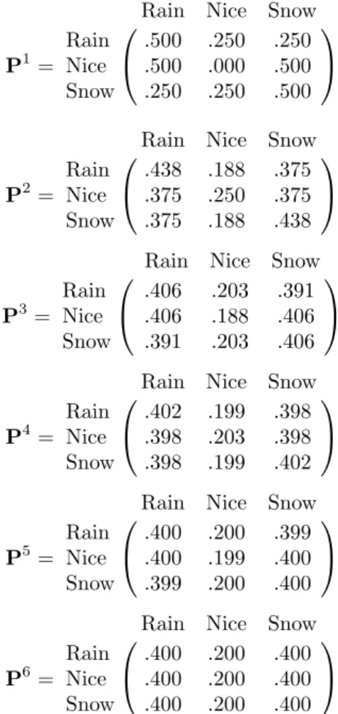
Example 11.2 (Example 11.1 continued) Consider again the weather in the Land of Oz. We know that the powers of the transition matrix give us interesting in-formation about the process as it evolves. We shall be particularly interested in the state of the chain after a large number of steps. The programMatrixPowers
computes the powers ofP.
We have run the programMatrixPowersfor the Land of Oz example to com-pute the successive powers ofPfrom 1 to 6. The results are shown in Table 11.1. We note that after six days our weather predictions are, to three-decimal-place ac-curacy, independent of today’s weather. The probabilities for the three types of weather, R, N, and S, are .4, .2, and .4 no matter where the chain started. This is an example of a type of Markov chain called a regular Markov chain. For this type of chain, it is true that long-range predictions are independent of the starting state. Not all chains are regular, but this is an important class of chains that we
shall study in detail later. 2
We now consider the long-term behavior of a Markov chain when it starts in a state chosen by a probability distribution on the set of states, which we will call a
probability vector. A probability vector with r components is a row vector whose entries are non-negative and sum to 1. Ifuis a probability vector which represents the initial state of a Markov chain, then we think of the ith component of u as representing the probability that the chain starts in statesi.
With this interpretation of random starting states, it is easy to prove the fol-lowing theorem.
P1=
Rain Nice Snow Rain .500 .250 .250 Nice .500 .000 .500 Snow .250 .250 .500
P2=
Rain Nice Snow Rain .438 .188 .375 Nice .375 .250 .375 Snow .375 .188 .438
P3=
Rain Nice Snow Rain .406 .203 .391 Nice .406 .188 .406 Snow .391 .203 .406
P4=
Rain Nice Snow Rain .402 .199 .398 Nice .398 .203 .398 Snow .398 .199 .402
P5=
Rain Nice Snow Rain .400 .200 .399 Nice .400 .199 .400 Snow .399 .200 .400
P6=
Rain Nice Snow Rain .400 .200 .400 Nice .400 .200 .400 Snow .400 .200 .400
11.1. INTRODUCTION 409
Theorem 11.2 LetPbe the transition matrix of a Markov chain, and letube the probability vector which represents the starting distribution. Then the probability that the chain is in statesi afternsteps is theith entry in the vector
u(n)=uPn .
Proof.The proof of this theorem is left as an exercise (Exercise 18). 2 We note that if we want to examine the behavior of the chain under the assump-tion that it starts in a certain state si, we simply choose uto be the probability
vector withith entry equal to 1 and all other entries equal to 0.
Example 11.3 In the Land of Oz example (Example 11.1) let the initial probability vectoruequal (1/3,1/3,1/3). Then we can calculate the distribution of the states after three days using Theorem 11.2 and our previous calculation ofP3. We obtain
u(3) =uP3 = ( 1/3, 1/3, 1/3 )
..406406 ..203188 ..391406
.391 .203 .406
= (.401, .188, .401 ) .
2
Examples
The following examples of Markov chains will be used throughout the chapter for exercises.
Example 11.4 The President of the United States tells person A his or her in-tention to run or not to run in the next election. Then A relays the news to B, who in turn relays the message to C, and so forth, always to some new person. We assume that there is a probabilityathat a person will change the answer from yes to no when transmitting it to the next person and a probability b that he or she will change it from no to yes. We choose as states the message, either yes or no. The transition matrix is then
P=
µ yes no
yes 1−a a
no b 1−b
.
The initial state represents the President’s choice. 2
Example 11.5 Each time a certain horse runs in a three-horse race, he has proba-bility 1/2 of winning, 1/4 of coming in second, and 1/4 of coming in third, indepen-dent of the outcome of any previous race. We have an indepenindepen-dent trials process,
but it can also be considered from the point of view of Markov chain theory. The transition matrix is
P=
W P S
W .5 .25 .25 P .5 .25 .25 S .5 .25 .25
.
2 Example 11.6 In the Dark Ages, Harvard, Dartmouth, and Yale admitted only male students. Assume that, at that time, 80 percent of the sons of Harvard men went to Harvard and the rest went to Yale, 40 percent of the sons of Yale men went to Yale, and the rest split evenly between Harvard and Dartmouth; and of the sons of Dartmouth men, 70 percent went to Dartmouth, 20 percent to Harvard, and 10 percent to Yale. We form a Markov chain with transition matrix
P=
H Y D
H .8 .2 0 Y .3 .4 .3 D .2 .1 .7
.
2 Example 11.7 Modify Example 11.6 by assuming that the son of a Harvard man always went to Harvard. The transition matrix is now
P=
H Y D
H 1 0 0
Y .3 .4 .3 D .2 .1 .7
.
2 Example 11.8 (Ehrenfest Model) The following is a special case of a model, called the Ehrenfest model,3that has been used to explain diffusion of gases. The general
model will be discussed in detail in Section 11.5. We have two urns that, between them, contain four balls. At each step, one of the four balls is chosen at random and moved from the urn that it is in into the other urn. We choose, as states, the number of balls in the first urn. The transition matrix is then
P=
0 1 2 3 4
0 0 1 0 0 0
1 1/4 0 3/4 0 0
2 0 1/2 0 1/2 0
3 0 0 3/4 0 1/4
4 0 0 0 1 0
.
2 3P. and T. Ehrenfest, “ ¨Uber zwei bekannte Einw¨ande gegen das Boltzmannsche H-Theorem,” Physikalishce Zeitschrift,vol. 8 (1907), pp. 311-314.
11.1. INTRODUCTION 411
Example 11.9 (Gene Model) The simplest type of inheritance of traits in animals occurs when a trait is governed by a pair of genes, each of which may be of two types, say G and g. An individual may have a GG combination or Gg (which is genetically the same as gG) or gg. Very often the GG and Gg types are indistinguishable in appearance, and then we say that the G gene dominates the g gene. An individual is called dominant if he or she has GG genes, recessive if he or she has gg, and
hybrid with a Gg mixture.
In the mating of two animals, the offspring inherits one gene of the pair from each parent, and the basic assumption of genetics is that these genes are selected at random, independently of each other. This assumption determines the probability of occurrence of each type of offspring. The offspring of two purely dominant parents must be dominant, of two recessive parents must be recessive, and of one dominant and one recessive parent must be hybrid.
In the mating of a dominant and a hybrid animal, each offspring must get a G gene from the former and has an equal chance of getting G or g from the latter. Hence there is an equal probability for getting a dominant or a hybrid offspring. Again, in the mating of a recessive and a hybrid, there is an even chance for getting either a recessive or a hybrid. In the mating of two hybrids, the offspring has an equal chance of getting G or g from each parent. Hence the probabilities are 1/4 for GG, 1/2 for Gg, and 1/4 for gg.
Consider a process of continued matings. We start with an individual of known genetic character and mate it with a hybrid. We assume that there is at least one offspring. An offspring is chosen at random and is mated with a hybrid and this process repeated through a number of generations. The genetic type of the chosen offspring in successive generations can be represented by a Markov chain. The states are dominant, hybrid, and recessive, and indicated by GG, Gg, and gg respectively.
The transition probabilities are
P=
GG Gg gg
GG .5 .5 0
Gg .25 .5 .25
gg 0 .5 .5
.
2 Example 11.10 Modify Example 11.9 as follows: Instead of mating the oldest offspring with a hybrid, we mate it with a dominant individual. The transition matrix is
P=
GG Gg gg
GG 1 0 0
Gg .5 .5 0
gg 0 1 0
.
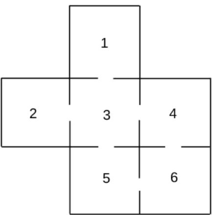
Example 11.11 We start with two animals of opposite sex, mate them, select two of their offspring of opposite sex, and mate those, and so forth. To simplify the example, we will assume that the trait under consideration is independent of sex.
Here a state is determined by a pair of animals. Hence, the states of our process will be: s1 = (GG,GG), s2 = (GG,Gg), s3 = (GG,gg), s4 = (Gg,Gg), s5 =
(Gg,gg), ands6= (gg,gg).
We illustrate the calculation of transition probabilities in terms of the states2.
When the process is in this state, one parent has GG genes, the other Gg. Hence, the probability of a dominant offspring is 1/2. Then the probability of transition to s1 (selection of two dominants) is 1/4, transition tos2 is 1/2, and to s4 is 1/4.
The other states are treated the same way. The transition matrix of this chain is:
P1=
GG,GG GG,Gg GG,gg Gg,Gg Gg,gg gg,gg
GG,GG 1.000 .000 .000 .000 .000 .000
GG,Gg .250 .500 .000 .250 .000 .000
GG,gg .000 .000 .000 1.000 .000 .000
Gg,Gg .062 .250 .125 .250 .250 .062
Gg,gg .000 .000 .000 .250 .500 .250
gg,gg .000 .000 .000 .000 .000 1.000
.
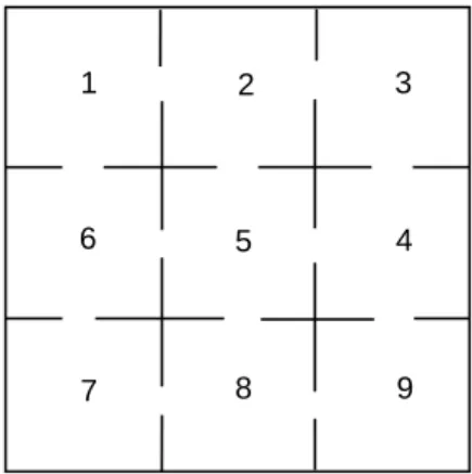
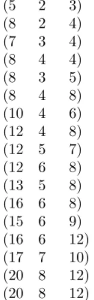
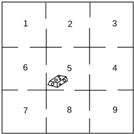
2 Example 11.12 (Stepping Stone Model) Our final example is another example that has been used in the study of genetics. It is called thestepping stone model.4 In this model we have an n-by-n array of squares, and each square is initially any one ofkdifferent colors. For each step, a square is chosen at random. This square then chooses one of its eight neighbors at random and assumes the color of that neighbor. To avoid boundary problems, we assume that if a square S is on the left-hand boundary, say, but not at a corner, it is adjacent to the squareT on the right-hand boundary in the same row asS, andSis also adjacent to the squares just above and belowT. A similar assumption is made about squares on the upper and lower boundaries. (These adjacencies are much easier to understand if one imagines making the array into a cylinder by gluing the top and bottom edge together, and then making the cylinder into a doughnut by gluing the two circular boundaries together.) With these adjacencies, each square in the array is adjacent to exactly eight other squares.
A state in this Markov chain is a description of the color of each square. For this Markov chain the number of states is kn2
, which for even a small array of squares is enormous. This is an example of a Markov chain that is easy to simulate but difficult to analyze in terms of its transition matrix. The programSteppingStone
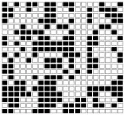
simulates this chain. We have started with a random initial configuration of two colors withn= 20 and show the result after the process has run for some time in Figure 11.2.
4S. Sawyer, “Results for The Stepping Stone Model for Migration in Population Genetics,” Annals of Probability,vol. 4 (1979), pp. 699–728.
11.1. INTRODUCTION 413
Figure 11.1: Initial state of the stepping stone model.
Figure 11.2: State of the stepping stone model after 10,000 steps.
This is an example of an absorbing Markov chain. This type of chain will be studied in Section 11.2. One of the theorems proved in that section, applied to the present example, implies that with probability 1, the stones will eventually all be the same color. By watching the program run, you can see that territories are established and a battle develops to see which color survives. At any time the probability that a particular color will win out is equal to the proportion of the array of this color. You are asked to prove this in Exercise 11.2.32. 2
Exercises
1 It is raining in the Land of Oz. Determine a tree and a tree measure for the next three days’ weather. Find w(1),w(2), and w(3) and compare with the
results obtained from P, P2, andP3.
2 In Example 11.4, let a= 0 andb = 1/2. Find P, P2, and P3. What would
Pn be? What happens toPn asntends to infinity? Interpret this result.
4 For Example 11.6, find the probability that the grandson of a man from Har-vard went to HarHar-vard.
5 In Example 11.7, find the probability that the grandson of a man from Harvard went to Harvard.
6 In Example 11.9, assume that we start with a hybrid bred to a hybrid. Find
w(1),w(2), andw(3).What wouldw(n) be?
7 Find the matrices P2, P3, P4,andPn for the Markov chain determined by the transition matrix P=
µ
1 0 0 1
. Do the same for the transition matrix
P=
µ
0 1 1 0
. Interpret what happens in each of these processes.
8 A certain calculating machine uses only the digits 0 and 1. It is supposed to transmit one of these digits through several stages. However, at every stage, there is a probability p that the digit that enters this stage will be changed when it leaves and a probabilityq= 1−pthat it won’t. Form a Markov chain to represent the process of transmission by taking as states the digits 0 and 1. What is the matrix of transition probabilities?
9 For the Markov chain in Exercise 8, draw a tree and assign a tree measure assuming that the process begins in state 0 and moves through two stages of transmission. What is the probability that the machine, after two stages, produces the digit 0 (i.e., the correct digit)? What is the probability that the machine never changed the digit from 0? Now letp=.1. Using the program
MatrixPowers, compute the 100th power of the transition matrix. Interpret the entries of this matrix. Repeat this withp=.2. Why do the 100th powers appear to be the same?
10 Modify the programMatrixPowers so that it prints out the averageAn of
the powersPn, forn= 1 toN. Try your program on the Land of Oz example and compareAn andPn.
11 Assume that a man’s profession can be classified as professional, skilled la-borer, or unskilled laborer. Assume that, of the sons of professional men, 80 percent are professional, 10 percent are skilled laborers, and 10 percent are unskilled laborers. In the case of sons of skilled laborers, 60 percent are skilled laborers, 20 percent are professional, and 20 percent are unskilled. Finally, in the case of unskilled laborers, 50 percent of the sons are unskilled laborers, and 25 percent each are in the other two categories. Assume that every man has at least one son, and form a Markov chain by following the profession of a randomly chosen son of a given family through several generations. Set up the matrix of transition probabilities. Find the probability that a randomly chosen grandson of an unskilled laborer is a professional man.
12 In Exercise 11, we assumed that every man has a son. Assume instead that the probability that a man has at least one son is .8. Form a Markov chain
11.2. ABSORBING MARKOV CHAINS 415 with four states. If a man has a son, the probability that this son is in a particular profession is the same as in Exercise 11. If there is no son, the process moves to state four which represents families whose male line has died out. Find the matrix of transition probabilities and find the probability that a randomly chosen grandson of an unskilled laborer is a professional man.
13 Write a program to compute u(n) given u and P. Use this program to
compute u(10) for the Land of Oz example, with u = (0,1,0), and with
u= (1/3,1/3,1/3).
14 Using the program MatrixPowers, find P1 throughP6 for Examples 11.9 and 11.10. See if you can predict the long-range probability of finding the process in each of the states for these examples.
15 Write a program to simulate the outcomes of a Markov chain after nsteps, given the initial starting state and the transition matrix P as data (see Ex-ample 11.12). Keep this program for use in later problems.
16 Modify the program of Exercise 15 so that it keeps track of the proportion of times in each state innsteps. Run the modified program for different starting states for Example 11.1 and Example 11.8. Does the initial state affect the proportion of time spent in each of the states if nis large?
17 Prove Theorem 11.1.
18 Prove Theorem 11.2.
19 Consider the following process. We have two coins, one of which is fair, and the other of which has heads on both sides. We give these two coins to our friend, who chooses one of them at random (each with probability 1/2). During the rest of the process, she uses only the coin that she chose. She now proceeds to toss the coin many times, reporting the results. We consider this process to consist solely of what she reports to us.
(a) Given that she reports a head on thenth toss, what is the probability that a head is thrown on the (n+ 1)st toss?
(b) Consider this process as having two states, heads and tails. By computing the other three transition probabilities analogous to the one in part (a), write down a “transition matrix” for this process.
(c) Now assume that the process is in state “heads” on both the (n−1)st and the nth toss. Find the probability that a head comes up on the (n+ 1)st toss.
(d) Is this process a Markov chain?
11.2
Absorbing Markov Chains
The subject of Markov chains is best studied by considering special types of Markov chains. The first type that we shall study is called anabsorbing Markov chain.
1 2 3
0 4
1 1
1/2 1/2 1/2
1/2 1/2 1/2
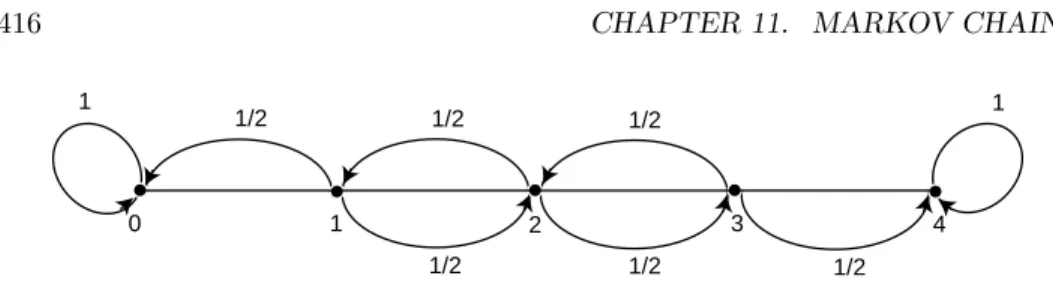
Figure 11.3: Drunkard’s walk.
Definition 11.1 A statesiof a Markov chain is calledabsorbing if it is impossible
to leave it (i.e.,pii= 1). A Markov chain isabsorbing if it has at least one absorbing
state, and if from every state it is possible to go to an absorbing state (not necessarily
in one step). 2
Definition 11.2 In an absorbing Markov chain, a state which is not absorbing is
calledtransient. 2
Drunkard’s Walk
Example 11.13 A man walks along a four-block stretch of Park Avenue (see Fig-ure 11.3). If he is at corner 1, 2, or 3, then he walks to the left or right with equal probability. He continues until he reaches corner 4, which is a bar, or corner 0, which is his home. If he reaches either home or the bar, he stays there.
We form a Markov chain with states 0, 1, 2, 3, and 4. States 0 and 4 are absorbing states. The transition matrix is then
P=
0 1 2 3 4
0 1 0 0 0 0
1 1/2 0 1/2 0 0
2 0 1/2 0 1/2 0
3 0 0 1/2 0 1/2
4 0 0 0 0 1
.
The states 1, 2, and 3 are transient states, and from any of these it is possible to reach the absorbing states 0 and 4. Hence the chain is an absorbing chain. When a process reaches an absorbing state, we shall say that it isabsorbed. 2 The most obvious question that can be asked about such a chain is: What is the probability that the process will eventually reach an absorbing state? Other interesting questions include: (a) What is the probability that the process will end up in a given absorbing state? (b) On the average, how long will it take for the process to be absorbed? (c) On the average, how many times will the process be in each transient state? The answers to all these questions depend, in general, on the state from which the process starts as well as the transition probabilities.
11.2. ABSORBING MARKOV CHAINS 417
Canonical Form
Consider an arbitrary absorbing Markov chain. Renumber the states so that the transient states come first. If there are r absorbing states and t transient states, the transition matrix will have the followingcanonical form
P =
TR. ABS.
TR. Q R
ABS. 0 I
Here Iis anr-by-rindentity matrix, 0is anr-by-tzero matrix, Ris a nonzero
t-by-r matrix, and Qis an t-by-t matrix. The first t states are transient and the lastrstates are absorbing.
In Section 11.1, we saw that the entryp(ijn)of the matrixPnis the probability of being in the statesjafternsteps, when the chain is started in statesi. A standard
matrix algebra argument shows thatPn is of the form
Pn =
TR. ABS.
TR. Qn ∗
ABS. 0 I
where the asterisk ∗ stands for the t-by-r matrix in the upper right-hand corner of Pn. (This submatrix can be written in terms of Q and R, but the expression is complicated and is not needed at this time.) The form of Pn shows that the entries ofQn give the probabilities for being in each of the transient states aftern
steps for each possible transient starting state. For our first theorem we prove that the probability of being in the transient states afternsteps approaches zero. Thus every entry of Qn must approach zero as napproaches infinity (i.e,Qn→ 0).
In the following, ifuandvare two vectors we say that u≤vif all components of u are less than or equal to the corresponding components of v. Similarly, if
Aand B are matrices thenA≤B if each entry ofA is less than or equal to the corresponding entry ofB.
Probability of Absorption
Theorem 11.3 In an absorbing Markov chain, the probability that the process will be absorbed is 1 (i.e.,Qn→0asn→ ∞).
Proof.From each nonabsorbing statesj it is possible to reach an absorbing state.
Let mj be the minimum number of steps required to reach an absorbing state,
starting from sj. Letpj be the probability that, starting fromsj, the process will
not reach an absorbing state inmj steps. Thenpj<1. Letmbe the largest of the
is less than or equal top, in 2nsteps less than or equal top2, etc. Sincep <1 these
probabilities tend to 0. Since the probability of not being absorbed inn steps is monotone decreasing, these probabilities also tend to 0, hence limn→∞Qn= 0. 2
The Fundamental Matrix
Theorem 11.4 For an absorbing Markov chain the matrixI−Q has an inverse
N and N=I+Q+Q2+· · · . The ij-entry nij of the matrixN is the expected
number of times the chain is in statesj, given that it starts in statesi. The initial
state is counted ifi=j.
Proof. Let (I−Q)x = 0; that is x = Qx. Then, iterating this we see that
x = Qnx.SinceQn →0, we have Qnx→0, so x = 0. Thus (I−Q)−1 = N
exists. Note next that
(I−Q)(I+Q+Q2+· · ·+Qn) =I−Qn+1 .
Thus multiplying both sides byN gives
I+Q+Q2+· · ·+Qn=N(I−Qn+1).
Lettingntend to infinity we have
N=I+Q+Q2+· · · .
Letsi andsj be two transient states, and assume throughout the remainder of
the proof that i and j are fixed. Let X(k) be a random variable which equals 1
if the chain is in state sj after k steps, and equals 0 otherwise. For each k, this
random variable depends upon bothiandj; we choose not to explicitly show this dependence in the interest of clarity. We have
P(X(k)= 1) =q(ijk) ,
and
P(X(k)= 0) = 1−qij(k) ,
where q(ijk) is the ijth entry ofQk. These equations hold for k= 0 since Q0 =I. Therefore, sinceX(k) is a 0-1 random variable,E(X(k)) =q(k)
ij .
The expected number of times the chain is in statesj in the firstnsteps, given
that it starts in statesi, is clearly
E
³
X(0)+X(1)+· · ·+X(n)
´
=qij(0)+qij(1)+· · ·+qij(n).
Lettingntend to infinity we have
E
³
X(0)+X(1)+· · ·
´
=q(0)ij +qij(1)+· · ·=nij .
11.2. ABSORBING MARKOV CHAINS 419
Definition 11.3 For an absorbing Markov chainP, the matrixN= (I−Q)−1 is
called thefundamental matrix forP. The entrynijofNgives the expected number
of times that the process is in the transient statesj if it is started in the transient
statesi. 2
Example 11.14 (Example 11.13 continued) In the Drunkard’s Walk example, the transition matrix in canonical form is
P =
1 2 3 0 4
1 0 1/2 0 1/2 0
2 1/2 0 1/2 0 0
3 0 1/2 0 0 1/2
0 0 0 0 1 0
4 0 0 0 0 1
.
From this we see that the matrixQis
Q=
10/2 1/02 10/2 0 1/2 0
,
and
I−Q=
−11/2 −11/2 −10/2
0 −1/2 1
.
Computing (I−Q)−1, we find
N= (I−Q)−1=
1 2 3
1 3/2 1 1/2
2 1 2 1
3 1/2 1 3/2
.
From the middle row of N, we see that if we start in state 2, then the expected number of times in states 1, 2, and 3 before being absorbed are 1, 2, and 1. 2
Time to Absorption
We now consider the question: Given that the chain starts in statesi, what is the
expected number of steps before the chain is absorbed? The answer is given in the next theorem.
Theorem 11.5 Lettibe the expected number of steps before the chain is absorbed,
given that the chain starts in state si, and let t be the column vector whose ith
entry isti. Then
t=Nc,
Proof. If we add all the entries in the ith row ofN, we will have the expected number of times in any of the transient states for a given starting state si, that
is, the expected time required before being absorbed. Thus, ti is the sum of the
entries in the ith row of N. If we write this statement in matrix form, we obtain
the theorem. 2
Absorption Probabilities
Theorem 11.6 Letbij be the probability that an absorbing chain will be absorbed
in the absorbing statesj if it starts in the transient state si. LetB be the matrix
with entriesbij. ThenBis ant-by-rmatrix, and
B=NR ,
whereN is the fundamental matrix andRis as in the canonical form.
Proof.We have
Bij =
X
n
X
k
q(ikn)rkj
= X
k
X
n
q(ikn)rkj
= X
k
nikrkj
= (NR)ij .
This completes the proof. 2
Another proof of this is given in Exercise 34.
Example 11.15 (Example 11.14 continued) In the Drunkard’s Walk example, we found that
N=
1 2 3
1 3/2 1 1/2
2 1 2 1
3 1/2 1 3/2
.
Hence,
t=Nc =
3/12 12 1/12 1/2 1 3/2
11
1
=
34
3
.
11.2. ABSORBING MARKOV CHAINS 421 Thus, starting in states 1, 2, and 3, the expected times to absorption are 3, 4, and 3, respectively.
From the canonical form,
R=
0 4
1 1/2 0
2 0 0
3 0 1/2
.
Hence,
B=NR =
3/12 12 1/12 1/2 1 3/2
·
1/02 00 0 1/2
=
0 4
1 3/4 1/4 2 1/2 1/2 3 1/4 3/4
.
Here the first row tells us that, starting from state 1, there is probability 3/4 of
absorption in state 0 and 1/4 of absorption in state 4. 2
Computation
The fact that we have been able to obtain these three descriptive quantities in matrix form makes it very easy to write a computer program that determines these quantities for a given absorbing chain matrix.
The programAbsorbingChaincalculates the basic descriptive quantities of an absorbing Markov chain.
We have run the programAbsorbingChainfor the example of the drunkard’s walk (Example 11.13) with 5 blocks. The results are as follows:
Q=
1 2 3 4
1 .00 .50 .00 .00 2 .50 .00 .50 .00 3 .00 .50 .00 .50 4 .00 .00 .50 .00
;
R=
0 5
1 .50 .00 2 .00 .00 3 .00 .00 4 .00 .50
;
N=
1 2 3 4
1 1.60 1.20 .80 .40 2 1.20 2.40 1.60 .80 3 .80 1.60 2.40 1.20 4 .40 .80 1.20 1.60
; t=
1 4.00 2 6.00 3 6.00 4 4.00
; B= 0 5
1 .80 .20 2 .60 .40 3 .40 .60 4 .20 .80
.
Note that the probability of reaching the bar before reaching home, starting at x, is x/5 (i.e., proportional to the distance of home from the starting point). (See Exercise 24.)
Exercises
1 In Example 11.4, for what values ofaandbdo we obtain an absorbing Markov chain?
2 Show that Example 11.7 is an absorbing Markov chain.
3 Which of the genetics examples (Examples 11.9, 11.10, and 11.11) are ab-sorbing?
4 Find the fundamental matrix Nfor Example 11.10.
5 For Example 11.11, verify that the following matrix is the inverse of I−Q
and hence is the fundamental matrix N.
N=
8/3 1/6 4/3 2/3 4/3 4/3 8/3 4/3 4/3 1/3 8/3 4/3 2/3 1/6 4/3 8/3
.
FindNcandNR. Interpret the results.
6 In the Land of Oz example (Example 11.1), change the transition matrix by making R an absorbing state. This gives
P=
R N S
R 1 0 0
N 1/2 0 1/2 S 1/4 1/4 1/2
.
11.2. ABSORBING MARKOV CHAINS 423 Find the fundamental matrixN, and alsoNcandNR. Interpret the results.
7 In Example 11.8, make states 0 and 4 into absorbing states. Find the fun-damental matrixN, and alsoNcandNR, for the resulting absorbing chain. Interpret the results.
8 In Example 11.13 (Drunkard’s Walk) of this section, assume that the proba-bility of a step to the right is 2/3, and a step to the left is 1/3. FindN, Nc, andNR. Compare these with the results of Example 11.15.
9 A process moves on the integers 1, 2, 3, 4, and 5. It starts at 1 and, on each successive step, moves to an integer greater than its present position, moving with equal probability to each of the remaining larger integers. State five is an absorbing state. Find the expected number of steps to reach state five.
10 Using the result of Exercise 9, make a conjecture for the form of the funda-mental matrix if the process moves as in that exercise, except that it now moves on the integers from 1 ton. Test your conjecture for several different values ofn. Can you conjecture an estimate for the expected number of steps to reach state n, for large n? (See Exercise 11 for a method of determining this expected number of steps.)
*11 Let bk denote the expected number of steps to reach n from n−k, in the
process described in Exercise 9.
(a) Defineb0= 0. Show that fork >0, we have
bk= 1 +
1
k
¡
bk−1+bk−2+· · ·+b0
¢
.
(b) Let
f(x) =b0+b1x+b2x2+· · · .
Using the recursion in part (a), show that f(x) satisfies the differential equation
(1−x)2y0−(1−x)y+ 1 = 0.
(c) Show that the general solution of the differential equation in part (b) is
y= −log(1−x)
1−x +
c
1−x ,
wherec is a constant. (d) Use part (c) to show that
bk = 1 +
1 2 +
1
3 +· · ·+ 1
k .
12 Three tanks fight a three-way duel. Tank A has probability 1/2 of destroying the tank at which it fires, tank B has probability 1/3 of destroying the tank at which it fires, and tank C has probability 1/6 of destroying the tank at which
it fires. The tanks fire together and each tank fires at the strongest opponent not yet destroyed. Form a Markov chain by taking as states the subsets of the set of tanks. Find N, Nc, and NR, and interpret your results. Hint: Take as states ABC, AC, BC, A, B, C, and none, indicating the tanks that could survive starting in state ABC. You can omit AB because this state cannot be reached from ABC.
13 Smith is in jail and has 3 dollars; he can get out on bail if he has 8 dollars. A guard agrees to make a series of bets with him. If Smith bets A dollars, he wins Adollars with probability .4 and loses Adollars with probability .6. Find the probability that he wins 8 dollars before losing all of his money if
(a) he bets 1 dollar each time (timid strategy).
(b) he bets, each time, as much as possible but not more than necessary to bring his fortune up to 8 dollars (bold strategy).
(c) Which strategy gives Smith the better chance of getting out of jail?
14 With the situation in Exercise 13, consider the strategy such that for i <4, Smith bets min(i,4−i), and fori≥4, he bets according to the bold strategy, where i is his current fortune. Find the probability that he gets out of jail using this strategy. How does this probability compare with that obtained for the bold strategy?
15 Consider the game of tennis whendeuceis reached. If a player wins the next point, he hasadvantage. On the following point, he either wins the game or the game returns to deuce. Assume that for any point, player A has probability .6 of winning the point and player B has probability .4 of winning the point. (a) Set this up as a Markov chain with state 1: A wins; 2: B wins; 3:
advantage A; 4: deuce; 5: advantage B. (b) Find the absorption probabilities.
(c) At deuce, find the expected duration of the game and the probability that B will win.
Exercises 16 and 17 concern the inheritance of color-blindness, which is a sex-linked characteristic. There is a pair of genes, g and G, of which the former tends to produce color-blindness, the latter normal vision. The G gene is dominant. But a man has only one gene, and if this is g, he is color-blind. A man inherits one of his mother’s two genes, while a woman inherits one gene from each parent. Thus a man may be of type G or g, while a woman may be type GG or Gg or gg. We will study a process of inbreeding similar to that of Example 11.11 by constructing a Markov chain.
16 List the states of the chain. Hint: There are six. Compute the transition probabilities. Find the fundamental matrixN, Nc, andNR.
11.2. ABSORBING MARKOV CHAINS 425
17 Show that in both Example 11.11 and the example just given, the probability of absorption in a state having genes of a particular type is equal to the proportion of genes of that type in the starting state. Show that this can be explained by the fact that a game in which your fortune is the number of genes of a particular type in the state of the Markov chain is a fair game.5
18 Assume that a student going to a certain four-year medical school in northern New England has, each year, a probabilityq of flunking out, a probability r
of having to repeat the year, and a probability p of moving on to the next year (in the fourth year, moving on means graduating).
(a) Form a transition matrix for this process taking as states F, 1, 2, 3, 4, and G where F stands for flunking out and G for graduating, and the other states represent the year of study.
(b) For the caseq=.1,r=.2, andp=.7 find the time a beginning student can expect to be in the second year. How long should this student expect to be in medical school?
(c) Find the probability that this beginning student will graduate.
19 (E. Brown6) Mary and John are playing the following game: They have a
three-card deck marked with the numbers 1, 2, and 3 and a spinner with the numbers 1, 2, and 3 on it. The game begins by dealing the cards out so that the dealer gets one card and the other person gets two. A move in the game consists of a spin of the spinner. The person having the card with the number that comes up on the spinner hands that card to the other person. The game ends when someone has all the cards.
(a) Set up the transition matrix for this absorbing Markov chain, where the states correspond to the number of cards that Mary has.
(b) Find the fundamental matrix.
(c) On the average, how many moves will the game last?
(d) If Mary deals, what is the probability that John will win the game?
20 Assume that an experiment hasmequally probable outcomes. Show that the expected number of independent trials before the first occurrence ofk consec-utive occurrences of one of these outcomes is (mk−1)/(m−1). Hint: Form an absorbing Markov chain with states 1, 2, . . . , k with state i representing the length of the current run. The expected time until a run of k is 1 more than the expected time until absorption for the chain started in state 1. It has been found that, in the decimal expansion of pi, starting with the 24,658,601st digit, there is a run of nine 7’s. What would your result say about the ex-pected number of digits necessary to find such a run if the digits are produced randomly?
5H. Gonshor, “An Application of Random Walk to a Problem in Population Genetics,” Amer-ican Math Monthly,vol. 94 (1987), pp. 668–671
21 (Roberts7) A city is divided into 3 areas 1, 2, and 3. It is estimated that
amounts u1, u2, andu3 of pollution are emitted each day from these three
areas. A fraction qij of the pollution from region i ends up the next day at
regionj. A fractionqi= 1−
P
jqij >0 goes into the atmosphere and escapes.
Letw(in) be the amount of pollution in areaiafterndays. (a) Show thatw(n)=u+uQ+· · ·+uQn−1.
(b) Show thatw(n)→w, and show how to computewfrom u.
(c) The government wants to limit pollution levels to a prescribed level by prescribing w. Show how to determine the levels of pollution u which would result in a prescribed limiting value w.
22 In the Leontief economic model,8 there are n industries 1, 2, . . . , n. The
ith industry requires an amount 0≤qij ≤1 of goods (in dollar value) from
companyj to produce 1 dollar’s worth of goods. The outside demand on the industries, in dollar value, is given by the vectord= (d1, d2, . . . , dn). Let Q
be the matrix with entriesqij.
(a) Show that if the industries produce total amounts given by the vector
x = (x1, x2, . . . , xn) then the amounts of goods of each type that the
industries will need just to meet their internal demands is given by the vectorxQ.
(b) Show that in order to meet the outside demand dand the internal de-mands the industries must produce total amounts given by a vector
x= (x1, x2, . . . , xn) which satisfies the equationx=xQ+d.
(c) Show that if Qis the Q-matrix for an absorbing Markov chain, then it is possible to meet any outside demand d.
(d) Assume that the row sums of Q are less than or equal to 1. Give an economic interpretation of this condition. Form a Markov chain by taking the states to be the industries and the transition probabilites to be theqij.
Add one absorbing state 0. Define
qi0= 1−
X
j
qij .
Show that this chain will be absorbing if every company is either making a profit or ultimately depends upon a profit-making company.
(e) Define xcto be the gross national product. Find an expression for the gross national product in terms of the demand vectordand the vector
tgiving the expected time to absorption.
23 A gambler plays a game in which on each play he wins one dollar with prob-abilitypand loses one dollar with probabilityq= 1−p. The Gambler’s Ruin
7F. Roberts,Discrete Mathematical Models (Englewood Cliffs, NJ: Prentice Hall, 1976). 8W. W. Leontief,Input-Output Economics(Oxford: Oxford University Press, 1966).
11.2. ABSORBING MARKOV CHAINS 427
problem is the problem of finding the probabilitywxof winning an amountT
before losing everything, starting with statex. Show that this problem may be considered to be an absorbing Markov chain with states 0, 1, 2, . . . ,T with 0 and T absorbing states. Suppose that a gambler has probability p= .48 of winning on each play. Suppose, in addition, that the gambler starts with 50 dollars and that T = 100 dollars. Simulate this game 100 times and see how often the gambler is ruined. This estimatesw50.
24 Show thatwxof Exercise 23 satisfies the following conditions:
(a) wx=pwx+1+qwx−1forx= 1, 2, . . . ,T−1.
(b) w0= 0.
(c) wT = 1.
Show that these conditions determine wx. Show that, ifp=q= 1/2, then
wx=
x T
satisfies (a), (b), and (c) and hence is the solution. If p6=q, show that
wx=
(q/p)x−1
(q/p)T −1
satisfies these conditions and hence gives the probability of the gambler win-ning.
25 Write a program to compute the probabilitywxof Exercise 24 for given values
ofx,p, andT. Study the probability that the gambler will ruin the bank in a game that is only slightly unfavorable, sayp=.49, if the bank has significantly more money than the gambler.
*26 We considered the two examples of the Drunkard’s Walk corresponding to the casesn= 4 andn= 5 blocks (see Example 11.13). Verify that in these two examples the expected time to absorption, starting atx, is equal tox(n−x). See if you can prove that this is true in general. Hint: Show that iff(x) is the expected time to absorption then f(0) =f(n) = 0 and
f(x) = (1/2)f(x−1) + (1/2)f(x+ 1) + 1
for 0 < x < n. Show that if f1(x) and f2(x) are two solutions, then their
differenceg(x) is a solution of the equation
g(x) = (1/2)g(x−1) + (1/2)g(x+ 1).
Also, g(0) =g(n) = 0. Show that it is not possible for g(x) to have a strict maximum or a strict minimum at the point i, where 1≤i≤n−1. Use this to show thatg(i) = 0 for all i. This shows that there is at most one solution. Then verify that the function f(x) =x(n−x) is a solution.
27 Consider an absorbing Markov chain with state space S. Letf be a function defined on S with the property that
f(i) =X
j∈S
pijf(j),
or in vector form
f=Pf.
Then f is called aharmonic function for P. If you imagine a game in which your fortune is f(i) when you are in state i, then the harmonic condition means that the game isfair in the sense that your expected fortune after one step is the same as it was before the step.
(a) Show that forf harmonic
f=Pnf
for alln.
(b) Show, using (a), that forf harmonic
f=P∞f,
where
P∞= lim
n→∞P
n =
µ
0 B
0 I
.
(c) Using (b), prove that when you start in a transient stateiyour expected
final fortune X
k
bikf(k)
is equal to your starting fortune f(i). In other words, a fair game on a finite state space remains fair to the end. (Fair games in general are called martingales. Fair games on infinite state spaces need not remain fair with an unlimited number of plays allowed. For example, consider the game of Heads or Tails (see Example 1.4). Let Peter start with 1 penny and play until he has 2. Then Peter will be sure to end up 1 penny ahead.)
28 A coin is tossed repeatedly. We are interested in finding the expected number of tosses until a particular pattern, say B = HTH, occurs for the first time. If, for example, the outcomes of the tosses are HHTTHTH we say that the pattern B has occurred for the first time after 7 tosses. LetTB be the time
to obtain pattern B for the first time. Li9 gives the following method for determiningE(TB).
We are in a casino and, before each toss of the coin, a gambler enters, pays 1 dollar to play, and bets that the pattern B = HTH will occur on the next
9S-Y. R. Li, “A Martingale Approach to the Study of Occurrence of Sequence Patterns in
11.2. ABSORBING MARKOV CHAINS 429 three tosses. If H occurs, he wins 2 dollars and bets this amount that the next outcome will be T. If he wins, he wins 4 dollars and bets this amount that H will come up next time. If he wins, he wins 8 dollars and the pattern has occurred. If at any time he loses, he leaves with no winnings.
Let A and B be two patterns. Let AB be the amount the gamblers win who arrive while the pattern A occurs and bet that B will occur. For example, if A = HT and B = HTH then AB = 2 + 4 = 6 since the first gambler bet on H and won 2 dollars and then bet on T and won 4 dollars more. The second gambler bet on H and lost. If A = HH and B = HTH, then AB = 2 since the first gambler bet on H and won but then bet on T and lost and the second gambler bet on H and won. If A = B = HTH then AB = BB = 8 + 2 = 10. Now for each gambler coming in, the casino takes in 1 dollar. Thus the casino takes in TB dollars. How much does it pay out? The only gamblers who go
off with any money are those who arrive during the time the pattern B occurs and they win the amount BB. But since all the bets made are perfectly fair bets, it seems quite intuitive that the expected amount the casino takes in should equal the expected amount that it pays out. That is,E(TB) = BB.
Since we have seen that for B = HTH, BB = 10, the expected time to reach the pattern HTH for the first time is 10. If we had been trying to get the pattern B = HHH, then BB = 8 + 4 + 2 = 14 since all the last three gamblers are paid off in this case. Thus the expected time to get the pattern HHH is 14. To justify this argument, Li used a theorem from the theory of martingales (fair games).
We can obtain these expectations by considering a Markov chain whose states are the possible initial segments of the sequence HTH; these states are HTH, HT, H, and∅, where∅is the empty set. Then, for this example, the transition matrix is
HTH HT H ∅
HTH 1 0 0 0
HT .5 0 0 .5
H 0 .5 .5 0
∅ 0 0 .5 .5
,
and if B = HTH, E(TB) is the expected time to absorption for this chain
started in state∅.
Show, using the associated Markov chain, that the values E(TB) = 10 and
E(TB) = 14 are correct for the expected time to reach the patterns HTH and
HHH, respectively.
29 We can use the gambling interpretation given in Exercise 28 to find the ex-pected number of tosses required to reach pattern B when we start with pat-tern A. To be a meaningful problem, we assume that patpat-tern A does not have pattern B as a subpattern. LetEA(TB) be the expected time to reach pattern
B starting with pattern A. We use our gambling scheme and assume that the first k coin tosses produced the pattern A. During this time, the gamblers
made an amount AB. The total amount the gamblers will have made when the pattern B occurs is BB. Thus, the amount that the gamblers made after the pattern A has occurred is BB - AB. Again by the fair game argument,
EA(TB) = BB-AB.
For example, suppose that we start with pattern A = HT and are trying to get the pattern B = HTH. Then we saw in Exercise 28 that AB = 4 and BB = 10 soEA(TB) = BB-AB= 6.
Verify that this gambling interpretation leads to the correct answer for all starting states in the examples that you worked in Exercise 28.
30 Here is an elegant method due to Guibas and Odlyzko10to obtain the expected
time to reach a pattern, say HTH, for the first time. Letf(n) be the number of sequences of lengthnwhich do not have the pattern HTH. Letfp(n) be the
number of sequences that have the pattern for the first time after n tosses. To each element of f(n), add the pattern HTH. Then divide the resulting sequences into three subsets: the set where HTH occurs for the first time at timen+ 1 (for this, the original sequence must have ended with HT); the set where HTH occurs for the first time at time n+ 2 (cannot happen for this pattern); and the set where the sequence HTH occurs for the first time at time
n+ 3 (the original sequence ended with anything except HT). Doing this, we have
f(n) =fp(n+ 1) +fp(n+ 3) .
Thus,
f(n) 2n =
2fp(n+ 1)
2n+1 +
23f
p(n+ 3)
2n+3 .
IfT is the time that the pattern occurs for the first time, this equality states that
P(T > n) = 2P(T =n+ 1) + 8P(T =n+ 3).
Show that if you sum this equality over all nyou obtain
∞
X
n=0
P(T > n) = 2 + 8 = 10.
Show that for any integer-valued random variable
E(T) =
∞
X
n=0
P(T > n),
and conclude that E(T) = 10. Note that this method of proof makes very clear that E(T) is, in general, equal to the expected amount the casino pays out and avoids the martingale system theorem used by Li.
10L. J. Guibas and A. M. Odlyzko, “String Overlaps, Pattern Matching, and Non-transitive
11.2. ABSORBING MARKOV CHAINS 431
31 In Example 11.11, definef(i) to be the proportion of G genes in statei. Show thatf is a harmonic function (see Exercise 27). Why does this show that the probability of being absorbed in state (GG,GG) is equal to the proportion of G genes in the starting state? (See Exercise 17.)
32 Show that the stepping stone model (Example 11.12) is an absorbing Markov chain. Assume that you are playing a game with red and green squares, in which your fortune at any time is equal to the proportion of red squares at that time. Give an argument to show that this is a fair game in the sense that your expected winning after each step is just what it was before this step.Hint: Show that for every possible outcome in which your fortune will decrease by one there is another outcome of exactly the same probability where it will increase by one.
Use this fact and the results of Exercise 27 to show that the probability that a particular color wins out is equal to the proportion of squares that are initially of this color.
33 Consider a random walker who moves on the integers 0, 1, . . . ,N, moving one step to the right with probabilitypand one step to the left with probability
q = 1−p. If the walker ever reaches 0 or N he stays there. (This is the Gambler’s Ruin problem of Exercise 23.) Ifp=qshow that the function
f(i) =i
is a harmonic function (see Exercise 27), and ifp6=qthen
f(i) =
µ
q p
¶i
is a harmonic function. Use this and the result of Exercise 27 to show that the probability biN of being absorbed in stateN starting in stateiis
biN =
( i
N, ifp=q,
(qp) i−
1
(qp)N−1, ifp6=q.
For an alternative derivation of these results see Exercise 24.
34 Complete the following alternate proof of Theorem 11.6. Let si be a
tran-sient state and sj be an absorbing state. If we compute bij in terms of the
possibilities on the outcome of the first step, then we have the equation
bij=pij+
X
k
pikbkj ,
where the summation is carried out over all transient statessk. Write this in
matrix form, and derive from this equation the statement
35 In Monte Carlo roulette (see Example 6.6), under option (c), there are six states (S,W,L,E, P1, and P2). The reader is referred to Figure 6.2, which
contains a tree for this option. Form a Markov chain for this option, and use the programAbsorbingChainto find the probabilities that you win, lose, or break even for a 1 franc bet on red. Using these probabilities, find the expected winnings for this bet. For a more general discussion of Markov chains applied to roulette, see the article of H. Sagan referred to in Example 6.13.
36 We consider next a game called Penney-ante by its inventor W. Penney.11
There are two players; the first player picks a pattern A of H’s and T’s, and then the second player, knowing the choice of the first player, picks a different pattern B. We assume that neither pattern is a subpattern of the other pattern. A coin is tossed a sequence of times, and the player whose pattern comes up first is the winner. To analyze the game, we need to find the probability pA
that pattern A will occur before pattern B and the probabilitypB = 1−pA
that pattern B occurs before pattern A. To determine these probabilities we use the results of Exercises 28 and 29. Here you were asked to show that, the expected time to reach a pattern B for the first time is,
E(TB) =BB ,
and, starting with pattern A, the expected time to reach pattern B is
EA(TB) =BB−AB .
(a) Show that the odds that the first player will win are given by John Conway’s formula12:
pA
1−pA
= pA
pB
= BB−BA
AA−AB .
Hint: Explain why
E(TB) =E(TAorB) +pAEA(TB)
and thus
BB=E(TAorB) +pA(BB−AB).
Interchange A and B to find a similar equation involving thepB. Finally,
note that
pA+pB = 1.
Use these equations to solve forpA andpB.
(b) Assume that both players choose a pattern of the same length k. Show that, if k = 2, this is a fair game, but, if k = 3, the second player has an advantage no matter what choice the first player makes. (It has been shown that, for k ≥ 3, if the first player chooses a1, a2, . . . , ak, then
the optimal strategy for the second player is of the formb,a1, . . . ,ak−1
whereb is the better of the two choices H or T.13)
11W. Penney, “Problem: Penney-Ante,”Journal of Recreational Math,vol. 2 (1969), p. 241. 12M. Gardner, “Mathematical Games,”Scientific American,vol. 10 (1974), pp. 120–125. 13Guibas and Odlyzko, op. cit.
11.3. ERGODIC MARKOV CHAINS 433
11.3
Ergodic Markov Chains
A second important kind of Markov chain we shall study in detail is an ergodic
Markov chain, defined as follows.
Definition 11.4 A Markov chain is called an ergodic chain if it is possible to go from every state to every state (not necessarily in one move). 2
In many books, ergodic Markov chains are called irreducible.
Definition 11.5 A Markov chain is called a regular chain if some power of the
transition matrix has only positive elements. 2
In other words, for some n, it is possible to go from any state to any state in exactly nsteps. It is clear from this definition that every regular chain is ergodic. On the other hand, an ergodic chain is not necessarily regular, as the following examples show.
Example 11.16 Let the transition matrix of a Markov chain be defined by
P=
µ1 2
1 0 1
2 1 0
.
Then is clear that it is possible to move from any state to any state, so the chain is ergodic. However, ifnis odd, then it is not possible to move from state 0 to state 0 innsteps, and ifnis even, then it is not possible to move from state 0 to state 1
innsteps, so the chain is not regular. 2
A more interesting example of an ergodic, non-regular Markov chain is provided by the Ehrenfest urn model.
Example 11.17 Recall the Ehrenfest urn model (Example 11.8). The transition matrix for this example is
P=
0 1 2 3 4
0 0 1 0 0 0
1 1/4 0 3/4 0 0
2 0 1/2 0 1/2 0
3 0 0 3/4 0 1/4
4 0 0 0 1 0
.
In this example, if we start in state 0 we will, after any even number of steps, be in either state 0, 2 or 4, and after any odd number of steps, be in states 1 or 3. Thus