COMPARING MANUAL AND AUTOMATIC NORMALIZATION
TECHNIQUES FOR RELATIONAL DATABASE
Sherry Verma *
ABSTRACT
Normalization is a process of analyzing the given relation schemas based on their Functional dependencies and primary keys to achieve the desirable properties of minimizing redundancy. It aims at creating a set of relational tables with minimum data redundancy that preserve consistency and facilitate correct insertion, deletion, and modification. A normalized database does not show various insertions, de letion and modification anomalies due to future updates. This paper presents a comparison study of manual and automatic normalization technique using sequential as well as parallel algorithm. It is very much time consuming to employ an automated technique to do this data analysis, as opposed to doing it manually. At the same time, the process is tested to be reliable and correct. It produces the dependency matrix and the directed graph matrix, first. It then proceeds with generating the 2NF, 3NF, and BCNF normal forms. All tables are also generated as the procedure proceeds.
Keywords: Automatic Normalization, Manual Normalization, Relational Database, Functional Dependency, and Primary Key.
1.
INTRODUCTION
Database normalization is the process of transforming data into well- formed or natural groupings such that one fact is stored in one place [1]. Normalization generally simplifies the relations and reduces the danger of anomalies [2] that may otherwise occur during manipulation of the relations in a relational database. Moreover, normalized data is stable and, therefore, provides a good foundation for any future growth. Thus, the normalization procedure provides database designers with a formal framework for analyzing relation schemas based on their keys and on the functional dependencies among their attributes [3]. It also provides a series of normal form tests that can be carried out on individual relation schemas so that the relational database can be normalized to any desired degree. E.F.Codd first formalized the process of normalization. It takes a relation schema through a series of tests to certify whether it satisfies a certain normal form. The normal form of a relation refers to the highest normal form condition that it meets, and hence indicates the degree to which it has been normalized. Three normal forms called first (1NF), second (2NF), and third (3NF) normal forms were initially proposed. An amendment was later added to the third normal form by R. Boyce and E.F. Codd called Boyce–Codd Normal Form (BCNF). The trend of defining other normal forms continued up to eighth normal form. In practice, however, databases are normalized up to and including BCNF. A relation is in first normal form if every field contains only atomic values, that is, no lists or sets, in the sense that it should not be able to be broken into more than one singleton value.Each normal form except the 1NF is defined on top of the previous normal form. That is, a table is said to be in 2NF if and only if it is in 1NF and it satisfies further conditions. Except for the 1NF, the other normal forms are based on Functional Dependencies (FD) among the attributes of a relation. A functional dependency (FD) is a constraint between two sets of attributes in a relation from a database [4]. Given a relation R, a set of attributes X in R is said to functionally determine another attribute Y, also in R, (written X → Y) if, and only if, each X value is associated with precisely one Y value.X is said to be the determinant set and Y the dependent set. Given that A, B, and C are sets of attributes in a relation R one can derive several properties of functional dependencies. Among the most important ones are Armstrong's axioms. These axioms are used in database normalization:
Axiom of Reflexivity: If B is a subset of A, then A -> B Axiom of Augmentation: If A -> C, then AB -> CB
Axiom of decomposition, or projection: If A -> BC, then A -> B and A -> C
Axiom of pseudotransitivity: If A->B, CB-> D, then AC -> D
Normalization is a major task in the design of relational databases [4]. Mechanism of the normalization process saves tremendous amount of time and money.
2.
TRADITIONAL
AND
AUTOMATIC
NORMALIZATION
TECHNIQUE
2.1 Traditional ApproachAs already mentioned, except the 1st normal form rest all normal forms depend upon FD’S. In the traditional method of normalizatio n we follow the abstract definitions of these normal forms and apply them to concrete problems [5]. To demonstrate this point, consider the following example, in which information concerning Suppliers, parts, and shipments is stored in a single relation:
First (S#, Status, City, P#, Quantity)
Here we assume that the relation is in 1st normal form. Now according to the definition of 2nd normal form, every non-prime attribute should be fully functional dependent on the primary key. So first to identify which attribute or combination of attribute makes primary key we need to run the following algorithm [6]:
A universal relation R and a set of FD’S F on attributes of R .To find key K
1. Set K: =R
2. For each attribute A in K {Compute (K-A)+ w.r.t F;
IF (K-A)+ contains all attributes in R, then set K: =K- {A}};
We found out that the combination of (S#, P#) makes the primary key of this relation. Our given relation violates the 2NF condition, as city and status are partially dependent on primary key, which will lead to redundancy as well as anomalies. So according to the rule we remove the partially dependent attributes from our original relation by decomposing it into two relations as follows:
First1 (S#, P#, Quantity)
First2 (S#, City, Status)
inserted until some supplier actually moves to that city (insertion anomaly). If only one supplier is in a city and that supplier is deleted, then the info rmation about the status of that city is lost (deletion anomaly). Finally, if the status for a specific city needs to be changed, every tuple for that city must be located and changed (updating anomaly). The reason for the danger of anomalies in First2 is the transitive dependency of status on S# via city. Each S# value determines a CITY value, and that CITY value determines the STATUS value. The solution to the problems is to decompose the First2 relation into two relations:
First21 (S#, City)
First22 (City, Status)
The above two relations are in 3NF. Moreover the decomposition is loss less and dependency preserving. Unfortunately, this traditional approach was difficult for many IS/IT students to grasp and/or apply the definitions. They cannot differentiate between the three normal forms and are confused about the relationships between FDs and normal forms. So Hsiang-Jui Kung and Han Reichgelt proposed an alternate method.
2.2 Automatic normalization approach using sequential algorithm
Like this many other approaches were being introduced. But despite normalization importance, very few algorithms have been developed to be used in the design of commercial Automatic normalization tools. Mathematical normalization algorithm is implemented in [8]. In [9] a set of stereotypes and tagged values are used to extend the UML meta- mode. A graph rewrite rule is then obtained to transfer the data model from one normal form to a higher normal form. Later on Amir Hassan Bahmani came up with the automatic database normalization technique, which use dependency graph diagrams to represent functional
key and all other attributes, which are transitively, depend on this key. For a relation with only one candidate key, 3NF and BCNF are equivalent. Let us take the previous example and solve it using the above- mentioned technique:
First (S#, Status, City, P#, Quantity)
S#, P# -> Quantity
City -> Status
S# -> City, Status
The graphical representation of the dependencies:
---
Fig1: Graphical representation of dependencies
If we are able to obtain all dependencies between determinant keys we can produce all dependencies between all attributes of a rela tion. These dependencies are represented by using a Dependency Matrix (DM). Using path finding algorithms and Armstrong’s
transitivity rule new dependencies are discovered from the existing dependency set. Dependency Matrix:
From a dependency graph, the corresponding Dependency Matrix (DM) is generated as follows:
i. Define matrix DM [n] [m], where n = number of Determinant Keys. m = number of Simple Keys.
S Status City P
SP
S P CITY STATUS QUANTITY
SP 2 2 0 0 1
CITY 0 0 2 1 0
S 2 0 1 1 0
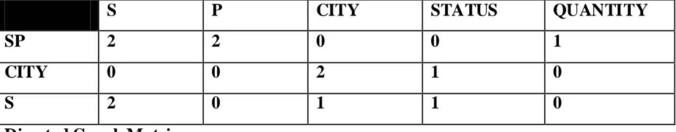
Directed Graph Matrix:
The Directed Graph (DG) matrix for determinant keys is used to represent all possible direct dependencies between determinant keys. The DG is an n×n matrix where n is the number of determinant keys. After running the algorithm for producing the DG graph, we get the following DG matrix:
SP CITY S
SP 1 - 1 1
CITY - 1 1 - 1
S - 1 1 1
After generating the DG matrix we turn our attention towards finding all possible paths between all pairs. This matrix will show all transitive dependencies between determinant keys. There is many such path finding algorithms like Prim, Kruskal, and Warshal algorithms. If there is a path from node x to node y it means y transitively depends on x.
SP CITY S
SP 1 - 1 1
CITY - 1 1 - 1
S - 1 1 1
Fig 2: Determinant key transitive dependencies
DM of Figure 2 is updated as follows to reflect all dependencies including those that are obtained by Dependency-closure procedure.
S P CITY STATUS QUANTITY
SP 2 2 S S 1
CITY 0 0 2 1 0
S 2 0 1 CITY 0
Fig 3: Dependency closure matrix
candidate key is a set of attributes to which all other attributes depend on. From the final DM we notice that SP has this property. This proposed 2NF and 3NF Normalization process makes use of both dependency and determinant key transitive dependencies. To proceed with the 2NF, it is assumed that the table is already in 1NF form. The resulting 1NF relation is: SP_Relation: {SP, City, Status, Quantity}
The goal is to discover all partial dependencies. To produce the 2NF form, we should find all partial dependencies. To do this, the DM is scanned row by row (ignoring the primary key row), starting from the first determinant key of the row being scanned are equal to 2 and the values of the corresponding columns of the candidate key are equal to 2, then a partial dependency is found. In Figure 3, the dependency of City to SP is partial.
row. Therefore, we have to create a new table. In Figure 4, the DM matrix is partitioned into two new DMs corresponding to new tables.
S P QUANTITY
SP 2 2 1
(a) SP_relation: {SP, Quantity}
S CITY STATUS
S 2 1 CITY
CITY 0 2 1
(b) S_relation: {S, City, Status}
Figure 4: Database normalized up to 2NF
In order to transform the relations into 3NF, each DM is scanned row by row starting from the first row. If a determinant key is encountered whose dependency is neither partial (from Figure 4) nor it is wholly dependent on part of the primary key a separate table has to be formed. Of course, if a table is previously formed a duplicate is not generated. This new table will include the determinant key and all other attributes, which are transitively, depend on this key.
S P QUANTITY
SP 2 2 1
(a)
S CITY
S 2 1
CITY STATUS
CITY 2 1
(c)
Figure 5 : Database Normalized up to 3NF
For a relation with only one candidate key, 3NF and BCNF are equivalent.
2.3 Automatic normalization approach using parallel algorithm
While existing sequential algorithms are usually much time consuming, especially the process of transforming relations into 3NF, so the proposed parallel algorithms for automatic database normalization was given. The proposed algorithms have been examined with MPI and its implementation results on EDM showed that parallel approach reduces the time, efficiently [11]. Exploiting p processors has reduced the time of Automatic Database
Normalization to c p
m n2.
in which c is the communication overhead between the
processors, m is the number of simple keys, and n is the number of determinant keys.
CONCLUSION
As we saw in traditional approach students need to remember the abstract definition of normal forms, moreover in some places canonical cover is supposed to be found out. This approach also requires finding out the primary key by applying algorithm, which again is a difficult job for students. Later automatic approach using both sequential and parallel algorithm were given. The process is based on the generation of dependency matrix, directed graph matrix, and determinant key transitive dependency matrix. The benefit of this approach over traditional approach is Primary Key is automatically identified for every final table that is generated. It is very much time consuming to employ an automated technique to do this data analysis, as opposed to doing it manually. At the same time, the sequential process is tested to be reliable and correct. The MPI implementation of (parallel algorithm for automatic database normalization) results on a cluster with eight processors indicates a considerable reduction in time of the automatic database normalization process. All these algorithms are very efficient. However, i will compare these algorithms with other similar algorithms, in the future.
REFERENCES
2. Kolahi, S., Dependency-Preserving Normalization of Relational and XML Data, Journal of Computer System Science, Vol. 73(4): pp. 636-647, 2007.
3. Ramez Elmasri and Shamkant B Navathe, Fundamentals Of Database Systems, 5th Edition,pg-358
4. Mora, A., M. Enciso, P. Cordero, IP de Guzman, An Efficient Preprocessing Transformation for Functional Dependencies Sets based on the Substitution Paradigm, CAEPIA2003, pp.136-146, 2003.
5. Kung, H. and T. Case, Traditional and Alternative Database Normalization Techniques: Their Impacts on IS/IT Students’ Perceptions and Performance,
International Journal of Information Technology Education, Vol.1, No.1 pp. 53-76,2004
6. Ramez Elmasri and Shamkant B Navathe, Fundamentals Of Database Systems, 5th Edition,pg-392
7. Date, C. J. (2000). An Introduction to Database Systems 7" Ed. Reading, MA: Addison-Wesley
8. Yazici, A., and Z. Karakaya, Normalizing Relational Database Schemas Using Mathematica, LNCS, Springer-Verlag, Vol.3992, pp. 375-382, 2006.
9. Akehurst, D.H., B. Bordbar, P.J. Rodgers, and N.T.G.Dalgliesh, Automatic Normalization via Metamodelling, ASE 2002 Workshop on Declarative Meta Programming to Support Software Development, 2002
10.A. H. Bahmani, M. Naghibzadeh, and B. Bahmani. Automatic database normalization and primary key generation. IEEE CCECE/CCGEI, pages 11–16, May 2008