Static and Incremental Overlapping Clustering Algorithms for Large
Collections Processing in GPU
Lázaro Janier González-Soler, Airel Pérez-Suárez and Leonardo Chang Advanced Technologies Application Center (CENATAV)
7ma A # 21406, Playa, CP: 12200, Havana, Cuba
E-mail: [email protected] and http://www.cenatav.co.cu/index.php/profile/profile/userprofile/jsoler E-mail: [email protected] and http://www.cenatav.co.cu/index.php/profile/profile/userprofile/asuarez E-mail: [email protected] and http://www.cenatav.co.cu/index.php/profile/profile/userprofile/lchang
Keywords:data mining, clustering, overlapping clustering, GPU computing
Received:November 18, 2016
Pattern Recognition and Data Mining pose several problems in which, by their inherent nature, it is con-sidered that an object can belong to more than one class; that is, clusters can overlap each other. OClustR and DClustR are overlapping clustering algorithms that have shown, in the task of documents clustering, the better tradeoff between quality of the clusters and efficiency, among the existing overlapping clustering algorithms. Despite the good achievements attained by both aforementioned algorithms, they areO(n2) so they could be less useful in applications dealing with a large number of documents. Moreover, although DClustR can efficiently process changes in an already clustered collection, the amount of memory it uses could make it not suitable for applications dealing with very large document collections. In this paper, two GPU-based parallel algorithms, named CUDA-OClus and CUDA-DClus, are proposed in order to enhance the efficiency of OClustR and DClustR, respectively, in problems dealing with a very large number of documents. The experimental evaluation conducted over several standard document collections showed the correctness of both CUDA-OClus and CUDA-DClus, and also their better performance in terms of efficiency and memory consumption.
Povzetek: OClustR in DClustR sta prekrivna algoritma za gruˇcenje, ki dosegata dobre rezultate, vendar je njuna kompleksnost kvadratnega reda velikosti. V tem prispevku sta predstavljena dva paralelna algo-ritma, ki temeljita na GPU: CUDA-OClus in CUDA-DClus. V eksperimentih sta pokazala zmožnost dela z velikimi koliˇcinami podatkov.
1
Introduction
Clustering is a technique of Machine Learning and Data Mining that has been widely used in several contexts [1]. This technique aims to structure a data set in clusters or classes such that objects belonging to the same class are more similar than objects belonging to different classes [2].
There are several problems that, by their inherent nature, consider that objects could belong to more than one class [3, 4, 5]; that is, clusters can overlap each other. Most of the clustering algorithms developed so far do not consider that clusters could share elements; however, the desire of ade-quately target those applications dealing with this problem, have recently favored the development ofoverlapping clus-tering algorithms;i.e., algorithms that allow objects to be-long to more than one cluster. An overlapping clustering algorithm that has shown, in the task of documents clus-tering, the better tradeoff between quality of the clusters and efficiency, among the existing overlapping clustering algorithms, is OClustR [6]. Despite the good achievements attained by OClustR in the task of documents clustering, it has two main limitations:
1. It has a computational complexity of O(n2), so it could be less useful in applications dealing with a large amount of documents.
2. It assumes that the entire collection is available be-fore clustering. Thus, when this collection changes it needs to rebuild the clusters starting from scratch; that is, OClustR does not use the previously built cluste-ring for updating the clusters after changes.
DClustR for storing the data it needs will also grow, ma-king DClustR a high memory consumer and consequently, making it not suitable for applications dealing with large collections. Motivated by the above mentioned facts, in this work we extend both OClustR and DClustR for efficiently processing very large document collections.
A technique that has been widely used in recent years in order to speed-up computing tasks is parallel computing and specifically, GPU computing. A GPU is a device that was initially designed for processing algorithms belonging to the graphical world, but due to its low cost, its high level of parallelism and its optimized floating-point operations, it has been used in many real applications dealing with a large amount of data.
The main contribution of this paper is the proposal of two GPU-based parallel algorithms, namely CUDA-OClusandCUDA-DClus, which enhance the efficiency of OClustR and DClustR, respectively, in problems dealing with a very large number of documents, like for instance news analysis, information organization and profiles iden-tification, among others.
Preliminary results of this paper were published in [8]. The main differences of this paper with respect to the conference paper presented in [8] are the following: (1) we introduce a new GPU-based algorithm, named CUDA-DClus, which is a parallel version of the DClustR algo-rithm, that is able to efficiently process changes in an alre-ady clustered collection and to efficiently process large col-lections of documents, and (2) we introduce a strategy for incrementally building and updating the connected compo-nents presented in a graph, allowing CUDA-DClus to mi-nimize the memory needed for processing the whole col-lection. It is important to highlight that in CUDA-DClus we only analyze the additions of objects to the collection, be-cause this is the case in which it could be difficult to apply DClustR in real applications dealing with large collections, since this is the case that makes the collection grow.
The remainder of this paper is organized as follows: in Section 2, a brief description of both the OClustR and DClustR algorithms are presented. In Section 3, the CUDA-OClus and CUDA-DClus parallel clustering algo-rithms are proposed. An experimental evaluation, showing the performance of both proposed algorithms on several document collections, is presented in Section 4. Finally, the conclusions as well as some ideas about future directi-ons are presented in Section 5.
2
OClustR and DClustR algorithms
In this section, both the OClustR [6] and DClustR [7] al-gorithms are described. Since DClustR is the extension of OClustR for efficiently processing collections that can change due to additions, deletions and modifications, the OClustR is first introduced and then, the strategy used by DClustR for updating the clustering after changes is pre-sented. All the definitions and examples presented in this
section were taken from [6, 7].
2.1
The OClustR algorithm
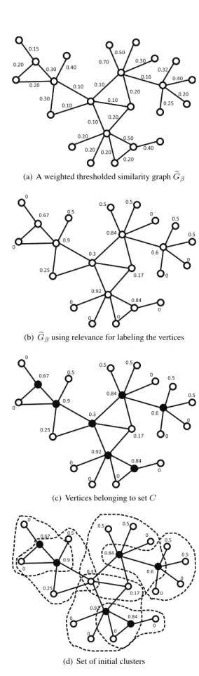
In order to build a set of overlapping clusters from a col-lection of objects, OClustR employs a strategy comprised of three stages. In the first stage, the collection of objects is represented by OClustR as aweighted thresholded simila-rity graph. Afterwards, in the second stage, an initial set of clusters is built through a cover of the graph representing the collection, using a special kind of subgraph. Finally, in the third stage the final set of overlapping clusters is obtai-ned by improving the initial set of clusters. Following, each stage is briefly described.
Let O = {o1, o2, . . . , on} be a collection of objects, β ∈[0,1]a similarity threshold, and S:O×O→ <a sym-metric similarity function. Aweighted thresholded simila-rity graph, denoted asGeβ =hV,Eeβ, Si, is an undirected
and weighted graph such thatV =Oand there is an edge
(v, u)∈EeβiffS(v, u)≥β; each edge(v, u)∈Eeβ, v6=u
is labeled with the value of S(v, u). As it can be infer-red, in the first stage OClustR must compute the similarity between each pair of objects; thus, the computational com-plexity of this stage isO(n2).
Once Geβ is built, in the second stage OClustR builds
an initial set of clusters through a covering ofGeβ, using weighted star-shaped sub-graphs.
LetGeβ =hV,Eeβ, Sibe a weighted thresholded
simila-rity graph. Aweighted star-shaped sub-graph(ws-graph) inGeβ, denoted by G? = hV?, E?, Si, is a sub-graph of
e
Gβ, having a vertexc∈V?, called thecenterofG?, such
that there is an edge betweencand all the other vertices in
V?\ {c}; these vertices are calledsatellites. All vertices in
e
Gβ having no adjacent vertices (i.e., isolated vertices) are
considereddegeneratedws-graphs.
For building a covering ofGeβusing ws-graphs, OClustR
must build a setW ={G?1, G?2, . . . , G?k}of ws-graphs of
e
Gβ, such thatV =Ski=1Vi?, beingVi?,∀i = 1. . . k, the
set of vertices of the ws-graphG?
i. For solving this
pro-blem, OClustR searches for a list C = {c1, c2, . . . , ck},
such thatci ∈ Cis the center ofGi? ∈ W,∀i = 1..k. In
the following, we will say that a vertexv iscoveredif it belongs toCor if it is adjacent to a vertex that belongs to
C. For pruning the search space and for establishing a cri-terion in order to select the vertices that should be included inC, the concept ofrelevanceof a vertex is introduced.
Therelevanceof a vertexv, denoted asv.relevance, is defined as the average between therelative densityand the
relative compactnessof a vertexv, denoted asv.densityR
andv.compactnessR, respectively, which are defined as follows:
v.densityR=|{u∈v.Adj/|v.Adj| ≥ |u.Adj|}|
|v.Adj| ,
v.compactnessR=|{u∈v.Adj/AIS(G
?
v)≥AIS(G ? u)}|
|v.Adj| ,
wherev.Adj andu.Adj are the set of adjacent vertices ofvandu, respectively;G?vandG?uare the ws-graphs
are theapproximated intra-cluster similarityofG?vandG?u,
respectively. Theapproximated intra-cluster similarityof a ws-graphG?is defined as the average weight of the edges
existing inG?between its center and its satellites.
Based on the above definitions, the strategy that OClustR uses in order to build the listCis composed of three steps. First, acandidate listLcontaining the vertices having rele-vance greater than zero is created; isolated vertices are di-rectly included inC. Then,Lis sorted in decreasing order of their relevance and each vertexv ∈Lis visited. Ifvis not covered yet or it has at least one adjacent vertex that is not covered yet, thenvis added toC. Each selected vertex, together with its adjacent vertices, constitutes a cluster in the initial set of clusters. The second stage of OClustR also has a computational complexity ofO(n2). Figure 1 shows through an example, the steps performed by OClustR in the second stage for building the initial set of clusters.
Finally, in the third stage, the final clusters are obtained though a process which aims to improve the initial clusters. With this aim, OClustR processesCin order to remove the vertices forming anon-usefulws-graph. A vertexvforms a non-useful ws-graph if: a) there is at least another ver-texu∈Csuch that the ws-graphudetermines includesv
as a satellite, andb) the ws-graph determined byv shares more vertices with other existing ws-graphs than those it only contains. For removing non useful vertices, OClustR uses three steps. First, the vertices inCare sorted in des-cending order according to their number of adjacent verti-ces. After that, each vertexv ∈ C is visited in order to remove those non-useful ws-graphs determined by vertices in(v.Adj∩C). If a ws-graphG?
u, withu∈(v.Adj∩C),
is non-useful,uis removed fromCand the satellites it only covers are “virtually linked” tov by adding them to a list namedv.Linked; in this way, those vertices virtually lin-ked to v will also belong to the ws-graph v determines. Once all vertices in(v.Adj∩C)are analyzed,vtogether with the vertices inv.Adjandv.Linkedconstitute a final cluster. This third stage also has a computational complex-ity ofO(n2). Figure 2 shows through an example, how the final clusters are obtained from the initial clusters showed in Figure 1(d).
2.2
Updating the clusters after changes: the
DClustR algorithm
Let Geβ = hV,Eeβ, Sibe the weighted thresholded
simi-larity graph that represents an already clustered collection
O. LetC = {c1, c2, . . . , ck} be the set of vertices
repre-senting the current covering ofGeβ and consequently, the
current clustering. When some vertices are added to and/or removed from O (i.e., fromGeβ), there could happen the
following two situations:
1) Some vertices become uncovered. This situation occurs when at least one of the added vertices is unco-vered or when those vertices ofCcovering a specific vertex were deleted fromGeβ.
0.15
0.20 0.30
0.20
0.40
0.30 0.10
0.10
0.10 0.10
0.10
0.20
0.20
0.20 0.20 0.50
0.40 0.20
0.16 0.30 0.50 0.70
0.32 0.40
0.20 0.25
0.20
(a) A weighted thresholded similarity graphGeβ
0
0
0.9 0.5
0.25
0.3
0.92 0.84
0
0 0
0.84
0 0.17
0.6 0 0.5 0.5
0.5
0
0 0.67
0.5
(b)Geβusing relevance for labeling the vertices
0
0
0.9 0.5
0.25
0.3
0.92 0.84
0
0
0.84 0 0.17
0.6 0 0.5 0.5
0.5
0
0 0.67
0
0.5
(c) Vertices belonging to setC
0
0
0.9 0.5
0.25
0.3
0.92 0.84
0 0
0.84 0 0.17
0.6 0 0.5 0.5
0.5
0 0 0.67
0
0.5
(d) Set of initial clusters
0
0
0.9 0.5
0.25
0.3
0.92 0.84
0 0
0.84 0 0.17
0.6 0 0.5 0.5
0.5
0 0 0.67
0
0.5
(a) Vertices determining non-useful ws-graphs (filled with light gray)
0
0
0.9 0.5
0.25
0.3
0.92 0.84
0 0
0.84 0 0.17
0.6 0 0.5 0.5
0.5
0 0 0.67
0
0.5
(b) Final set of overlapping clusters
Figure 2: Illustration of how the final clusters are obtained by OClustR in the third stage.
2) The relevance of some vertices changes and, as a con-sequence, at least one vertexu /∈Cappears such that
uhas relevance greater than at least one vertex inC
that covers vertices in u.Adj∪ {u}. Vertices likeu
could determine ws-graphs with more satellites and less overlapping with other graphs than other ws-graphs currently belonging to the covering ofGeβ.
Figure 3, illustrates the above commented situations over the graphGeβof Figure 1(a). Figure. 3(a), shows the graph
e
Gβbefore the changes; the vertices to be removed are
mar-ked with an “x”. Figure 3(b), shows graph Geβ after the
changes; vertices filled with light gray represent the added vertices. Figures 3(c) and 3(d), show the updated graph
e
Gβ with vertices labeled with letters and with their
up-dated value of relevance, respectively; vertices filled with black correspond with those vertices currently belonging to
C. As it can be seen from Figures 3(c) and 3(d), vertices
S, F, G, I, H andJ became uncovered after the changes, while vertex B, which does not belong to C, has a rele-vance greater than vertexD, which already belongs toC.
Taking into account the above mentioned situations, in order to update the clustering after changes DClustR first detects which are the connected components of Geβ that
were affected by changes and then it iteratively updates the covering of these components and consequently, their
clus-0.15
0.20 0.30
0.20
0.40
0.30 0.10
0.10
0.10 0.10
0.10
0.20
0.20
0.20 0.20
0.50 0.40 0.20
0.16 0.30 0.50 0.70
0.32 0.40
0.20 0.25
0.20 x
x
x x
x
(a)Geβbefore the changes
0.15
0.20 0.30
0.20
0.30
0.40 0.16 0.30 0.50
0.32 0.40
0.20 0.25
0.20 0.21
(b)Geβafter the changes
A
C B
D
E
F
G H
J K
M L
N
O
P Q
I S
R
(c)Geβwith vertices labeled with letters
0
0
0.88
0.67
0.5
0
0
0.75 0.5 0.67
0 0.5
0.5
0.5
0 0
0 0
0.7
(d) Geβ with vertices labeled with their updated value
of relevance
tering.
The connected components that are affected by changes are those that contain vertices that were added or verti-ces that were adjacent to vertiverti-ces that were deleted from
e
Gβ. Since DClustR has control over these vertices it can
build these components through a depth first search, star-ting from any of these vertices. Let G0 = hV0, E0, Sibe a connected component affected by changes, whose cove-ring must be updated. Let C0 ⊆ C be the set of vertices of G0 which determine ws-graphs (i.e., clusters) covering
G0. DClustR follows the same principles of OClustR; that is, it first builds or completes the covering ofG0in order to
build an initial set of clusters (stage 1) and then, it impro-ves these clusters in order to build the final set of clusters ofG0 (stage 2). In fact, DClustR uses the same steps that OClustR for the above two mentioned stages, but unlike OClustR, DClustR modifies the way in which the candi-date listL, used in stage 1, is built.
In order to build candidate listL, DClustR first recom-putes the relevance value of all vertices inG0and it empties the listc.Linked, for all verticesc∈C0; this last action is
supported by the fact that, after changes, there could be ws-graphs that were considered as non useful, which could be no longer so. LetV+ ⊆(V0\C0)be the set of vertices of
G0 with relevance greater than zero, which do not belong toC0. For building the candidate listL, bothC0andV+are processed.
For processingV+, DClustR visits each vertexv ∈V+ and it verifiesa) ifvis uncovered, orb) if at least one ad-jacent vertex ofvis uncovered, orc) if there is at least one vertexu∈v.Adj, such that there is no other vertex inC0
coveringuwhose relevance is greater than or equal to the relevance ofv. If any of these three conditions is fulfilled,
v is added toL. Additionally, if the last condition is ful-filled, all those vertices likeuare marked as “activated” in order to use them whenC0is being processed. The compu-tational complexity of the processing ofV+isO(n2).
For processingC0, DClustR visits the adjacent vertices of each vertexv∈C0. Any vertexu∈v.Adjhaving
grea-ter relevance thanvis added toL; in these cases,vis addi-tionally marked as “weak”. Once all the adjacent vertex of
vwere visited, ifvwas marked as “weak” or at least one of its adjacent vertices were previously marked as “active”,v
is removed fromC0since it could be substituted by a more relevant vertex. However, ifvhas a relevance greater than zero, it is still considered as a candidate and consequently, it is added toL. The computational complexity of the pro-cessing ofC0isO(n2).
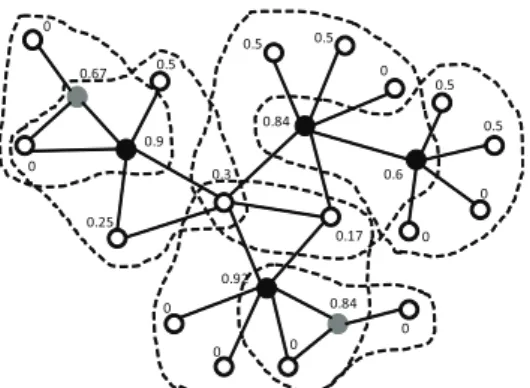
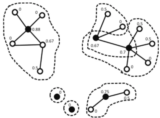
Figure 4, shows the updated set of overlapping clusters obtained by DClustR when it processes the graph in Fi-gure 3(d); vertices filled with black represent the vertices determining ws-graphs that cover each connected compo-nent ofGeβ.
Like OClustR, the computational complexity of DClustR isO(n2).
0
0 0.88
0.67
0.5
0
0
0.75 0.5 0.67
0 0.5
0.5
0.5
0
0
0 0
0.7
Figure 4: Updated set of overlapping clusters obtained by DClustR.
3
Proposed parallel algorithms
As it was mentioned in Section 1, despite the good achie-vements attained by OClustR and DClustR in the task of documents clustering, these algorithms areO(n2)so they could be less useful in applications dealing with a very large number of documents. Motivated by this fact, in this section two massively parallel implementations in CUDA of OClustR and DClustR are proposed in order to enhance the efficiency of OClustR and DClustR in the above menti-oned problems. These parallel algorithms, namely CUDA-OClusandCUDA-DClus, take advantage of the benefits of GPUs, like for instance, the high bandwidth communica-tion between CPU and GPU, and the GPU memory hierar-chy.
Although in their original articles both OClustR and DClustR were proposed as general purpose clustering al-gorithms, the parallel extensions proposed in this work are specifically designed for processing documents. This ap-plication context is the same in which both OClustR and DClustR were evaluated and it is also a context in which very large collections are commonly processed. In the context of document processing, both CUDA-OClus and CUDA-DClus use the cosine measure [9] for computing the similarity between two documents; this measure is the function that has been used the most for this purpose [10]. The cosine measure between two documentsdi anddj is
defined as:
cos(di, dj) =
Pm
k=1di(k)∗dj(k)
kdik · kdjk
, (1)
wheredi(k)anddj(k)are the weights of thekterm in the
description of the documentsdi anddj, respectively;kdik
andkdjkare the norms of documentsdi anddj,
respecti-vely.
by CUDA-OClus; remaining steps are high memory con-suming tasks that are more favored with a CPU implemen-tation. Analogously, in these experiments it was also ve-rified that the most time consuming steps of DClustR are the updating of the graph after changes and the recompu-ting of the relevance, so these steps will be implemented in CUDA by CUDA-DClus. In this case, it could be no-ticed also that the detection of the connected components affected by changes is a high memory consuming task per-formed by DClustR, so it is also important to address this problem in CUDA-DClus.
Finally, it is also important to mention that since we are dealing with the problem of processing very large do-cument collections, CUDA-DClus only tackles additions, which are the changes that could increase the size of the collection. Implementing deletions is irrelevant for overco-ming problems related with large document collections.
Following, the CUDA-OClus algorithm is first introdu-ced and then, the CUDA-DClust algorithm is presented.
3.1
CUDA-OClus algorithm
LetD={d1, d2. . . , dn}be a collection of documents
des-cribed by a set of terms. LetT = {t1, t2, . . . , tm}be the
list containing all the different terms that describe at least one document inD. CUDA-OClus represents a document
di ∈D by two parallel vectors, denoted byTdi andWdi.
The first one contains the position that the terms describing
dihave inT, and the second one contains the weights that
those terms have in the description ofdi.
For buildingGeβ = hV,Eeβ, Si, OClustR demandsSto
be a symmetric similarity measure, so the similarity bet-ween any two documents (i.e., vertices inGeβ) needs to be
computed only once. Based on this fact and considering the inherent order the documents have inside a collection
D(i.e., vertices inV), for building the edges relatives to a vertexv∈V it is only necessary to compute the similarity betweenvand each vertex followingvinV. LetSucvbe
the list of vertices that follow a vertex v inV. To speed up the construction ofGeβ, for each vertexv ∈V,
CUDA-OClus will compute in parallel the similarity betweenvand the vertices inSucv.
Considering the definition of the cosine measure, it can be seen from Expression (1) that its numerator is a sum of independent products which could be computed all at once. On the other hand, taking into account that the norm of a document can be computed while the document is being read, the denominator of Expression (1) can be also resol-ved with no extra time. Based on these facts, CUDA-OClus also parallelizes the computation of the similarity between a pair of vertices, in order to speed up even more the con-struction ofGeβ.
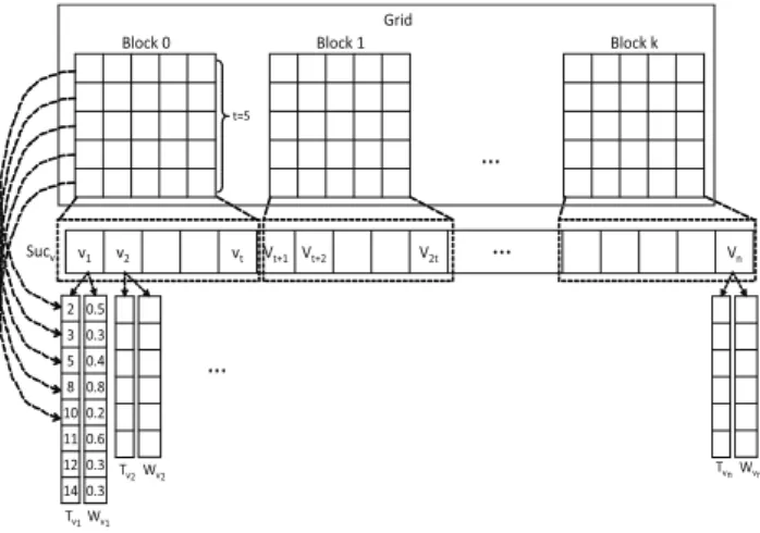
In order to carry out the previous idea, CUDA-OClus builds a grid comprised of k square blocks, each block having a shared memory square matrix (SMM); where
k = nt + 1andtis the dimension of both the blocks and the matrices. Agridis a logic representation of a matrix
of threads in the GPU. The use of SMM and its low la-tency will allow CUDA-OClus to not constantly access the CPU memory, speeding up the calculus of the similarity between two vertices. CUDA-OClus assigns totthe maxi-mum value allowed by the architecture of the GPU for the dimension of a SMM.
When CUDA-OClus is going to compute the similarity between a vertexvand the vertices inSucv, it first builds
a vectorPvof sizem. This vector has zero in all its entries
excepting in those expressed by the positions stored inTv;
these last entries contain their respective weights stored in
Wv. OncePv has been built, the listSucv is partitioned
intoksublists. Each one of these sublists is assigned to a block constituting the grid and the SMM associated with that block is emptied; i.e., all its cells are set to zero. When a sublistQ = {v1, v2, . . . , vp} is assigned to a block
in-side a grid, each vertex inQis assigned to a column of the block. In this context, to assign a vertexvito a column
me-ans that each row of the column points to a term describing
vi; in this way, thejth row points to thejth term
descri-bingvi. Figure 5 shows an example of how the listSucvis
divided by CUDA-OClus intoksublists and how these su-blists are assigned to the blocks constituting the grid. The example on Figure 5 shows how the first vertex of the su-blist assigned to “block 0” is assigned to the first column of that block; the other assignments could be deduced from this example.
…
Block 0 Block 1 Block k
Grid
2
3
5
8
10
11
12
14
v1 v2 vt Vt+1 Vt+2 V2t Vn
Sucv
0.5
0.3
0.4
0.8
0.2
0.6
0.3
0.3
Tv1Wv1
Tv2Wv2
…
…
T
vnWvn
t=5
Figure 5: Illustration of how CUDA-OClus dividesSucv
and assigns each resulting sublist to the blocks.
Each row inside a column of a block has a thread that performs a set of operations. In our case, the threads asso-ciated with theith column will compute the similarity bet-weenvand its assigned vertexvi. With this aim, the thread
associated with each row inside theith column will com-pute the product between the weight that the term pointed by that row has in the description ofvi, and the weight this
by both documents; this is the reason we only use the terms ofviand multiply their weights by the weights that these
terms have inv; remaining terms invare useless.
Given that thejth row of the column to which vertexvi
has been assigned, points to thejth term ofTvi, the weight
this term has invi is stored at thejth position ofWviand
the weight this same term has inv is stored atPv, in the
entry referred by the value stored at thejth position ofTvi.
The result of the product between the above mentioned weights is added to the value the jth row already has in the SMM. If the description of a vertexvi assigned to a
column of a block exceeds the length of the column (i.e.,
t) atilingis applied at this block. Tiling [11] is a technique that consists on dividing a data set into a number of small subsets, such that each subset fits into the block; i.e., the SMM. Thus, when the rows of a column point at the nextt
terms, the products between the weights these terms have in the description ofvi andv are computed and
accumu-lated into the values these rows have in the SMM. This technique is applied until all the terms describing the verti-ces assigned to the columns have been proverti-cessed. Figure 6 shows how the similarity between the vertexv1 assigned to the first column of “Block 0” and v is computed. In this example, it has been assumed that there are 15 terms describing the documents of the collection, the size of the block is k = 5, and Tv = {1,2,5,8,10,12,14}, Wv = {0.2,0.6,0.3,0.7,0.2,0.1,0.5}, Tv1 = {2,3,5,8,10,11,12,14} and Wv1 =
{0.5,0.3,0.4,0.8,0.2,0.6,0.3,0.3}.
As it can be seen from Figure 6(a), each thread of thet
rows of the first column computes the product between the weight of the term it points at, and the weight this same term has inPv(i.e., the description ofv). As it was
menti-oned before, the computed products are stored in the SMM of that block. Note from Figure 6(a) that the product com-puted by the second row is zero since vertex v does not contain the term pointed out by this row; i.e., term having index 3rd inT. Figure 6(b) shows how when Tiling is ap-plied, the remaining terms describingv1are pointed by the rows of the first column. Figure 6(c) shows how the pro-ducts between the remaining terms ofv1andvare perfor-med. Finally, Figure 7 shows which are the values stored in the first column of the SMM of “Block 0”, once all the products have been computed.
Once all the terms describing the vertices assigned to a block have been processed, areductionis applied over each column of the block. Reduction [12] is an operation that computes in parallel the sum of all the values of a column of the SMM and then, it stores this sum in the first row of the column. Figure 8 shows the final sum obtained for the first column of “Block 0”.
The sum obtained on the column to with vertexvi has
been assigned corresponds with the numerator of the co-sine measure betweenv andvi. This sum is then divided
by the product of the norms ofvandvi, which have been
previously computed; the result of this division (i.e., the si-milarity betweenvandvi) is copied to the CPU. Using this
0.3 0 0.12 0.56 0.4 Block 0 0 1 2 3 4 5 6 7 8 9 10 11 12 13 14 Pv
v1 v2 vt
Sucv
T v2Wv2
… 0 0.2 0.6 0 0 0.3 0 0 0.7 0 0.2 0 0.1 0 0.5 t=5 2 3 5 8 10 11 12 14 0.5 0.3 0.4 0.8 0.2 0.6 0.3 0.3 T
v1Wv1
(a) Computing the firsttproducts
0 1 2 3 4 5 6 7 8 9 10 11 12 13 14 Pv 0 0.2 0.6 0 0 0.3 0 0 0.7 0 0.2 0 0.1 0 0.5 0.3 0 0.12 0.56 0.4 Block 0
v1 v2 vt
Sucv
T
v2Wv2
… t=5 2 3 5 8 10 11 12 14 0.5 0.3 0.4 0.8 0.2 0.6 0.3 0.3 T
v1Wv1 (b) ApplyingTiling
0 1 2 3 4 5 6 7 8 9 10 11 12 13 14 Pv 0 0.2 0.6 0 0 0.3 0 0 0.7 0 0.2 0 0.1 0 0.5 0.3 0 0.12 0.56 0.4
v1 v2 vt
Sucv
Tv2Wv2
… t=5 2 3 5 8 10 11 12 14 0.5 0.3 0.4 0.8 0.2 0.6 0.3 0.3 Tv1Wv1
Block 0
(c) Computing remaining products
Figure 6: Illustration of how CUDA-OClus computes the similarity between a vertexvand the vertices inSucv.
result CUDA-OClus decides if it should create or not an edge betweenvandvi, during this step CUDA-OClus also
0 1 2 3 4 5 6 7 8 9 10 11 12 13 14
Pv
0 0.2 0.6 0 0 0.3 0 0 0.7 0 0.2 0 0.1 0 0.5
0.3 0.03 0.27 0.56 0.4
v1 v2 vt
Sucv
T
v2Wv2
… t=5
2 3 5 8 10 11 12 14
0.5 0.3 0.4 0.8 0.2 0.6 0.3 0.3 T
v1Wv1
Block 0
Figure 7: Final results stored in the SMM after processing all terms ofv1.
0
1
2
3
4
5
6
7
8
9
10
11
12
13
14
Pv
0
0.2
0.6
0
0
0.3
0
0
0.7
0
0.2
0
0.1
0
0.5
1.56
v1 v2 vt
Sucv
Tv2Wv2
…
t=5
2
3
5
8
10
11
12
14 0.5
0.3
0.4
0.8
0.2
0.6
0.3
0.3
Tv1Wv1
Block 0
Figure 8: Result of applying Reduction on the first column of “Block 0”.
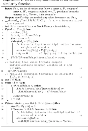
The pseudocode of cosine similarity function is shown in Algorithm 1.
Once the thresholded similarity graphGeβhas been built,
CUDA-OClus speeds up the computation of the other time-consuming step: the computation of the relevance of the vertices. In order to do that, CUDA-OClus computes in pa-rallel the relevance of all the vertices ofGeβ. Moreover, for
each vertexv, CUDA-OClus computes in parallel the con-tribution each adjacent vertex ofvhas over the relevance of
v, speeding up even more the computation of the relevance ofv. In order to accomplish this idea, the list of vertices of
e
Gβis partitioned intoksublists and each sublist is assigned
to a block inside a grid. However, in this case, when a ver-texviof a sublist is assigned to a column of a block, each
row in that column will point to an adjacent vertex ofvi;
e.g., thejth row points at thejth adjacent vertex ofvi.
Dif-Algorithm 1:CUDA implementation of the cosine similarity function.
Input:Sucvthe list of vertices that follow a vertexv,Pvweights of
vertexv,Wvweights associated tov,Tvposition of terms that
represent tov,N ormvis the norm ofv
Output:similarity: cosine similarity values betweenvandSucv
1 __shared__f loat SM M[R][C]; // R = C because block are squared
2 int tid=threadIdx.x+blockDim.x∗blockIdx.x; 3 if(tid <|Sucv|)then
4 u=Sucv[tid];
5 int tidy=threadIdx.y;
6 f loat sum= 0; 7 while(tidy<|Wu|)do
/* Accumulating the multiplication between
weights of v and u */
8 sum+=Wu[tidy]∗Pv[Tu[tidy]];
9 tidy+=R; // Applying tiling technique
10 SM M[threadIdx.y][threadIdx.x] =sum;
/* Waiting that whole threats compute multiplications between weights of v and
u∈Sucv */
11 __syncthreads();
/* Applying reduction technique to calculate
Pm
k=1di(k)∗dj(k) */ 12 int i=R/2;
13 while(i! = 0)do
14 if(threadIdx.y < i)then
15 SM M[threadIdx.y][threadIdx.x]+= SM M[threadIdx.y+i][threadIdx.x]; 16 __syncthreads();
17 i=i/2;
18 if(threadIdx.y== 0 &&tid <|Sucv|)then
19 similarity[tid] = 0;
20 if(N ormv>0 &&N ormu>0)then
/* Dividing between the multiplication of
norms of v and u */
21 similarity[tid] =
SM M[0][threadIdx.x]/(N ormv∗N ormu)
ferent from building graphGeβ, now the threads associated
with a column will compute the relevance of its assigned vertex. With this aim, the thread on each row of that co-lumn will compute the contributions the vertex pointed by that row has over the relevance of the vertex assigned to the column.
Letvbe a vertex assigned to a column anduone of its adjacent vertices. Vertexucontributes |v.Adj1 | to the rele-vance of vif |v.Adj| ≥ |u.Adj|; otherwise, its contribu-tion is zero. This case represents the contribucontribu-tionuhas to the relevance of v through the relative density of v. On the other hand, ucontributes |v.Adj1 | to the relevance ofv
ifAIS(v)≥ AIS(u); otherwise, its contribution is zero. This other case represents the contributionuhas to the re-levance ofv through the relative compactness of v. The total contribution provided by a vertex is added to the va-lue the row already has in the SMM; similar to the case of building graphGeβ, the SMM of each block is initially
emp-tied. Ifvhas more thantadjacent vertex, a Tiling is app-lied. Once all the adjacent vertices ofvhas been processed, a Reduction is applied in order to compute the relevance of
v. Obtained values are then copied to the CPU.
The pseudocode of cosine similarity function is shown in Algorithm 2.
Algorithm 2: CUDA implementation of the rele-vance function.
Input:Geβweights threshold similarity graph,AIS(Geβ)is the
approximated intra-cluster similarity ofGeβ
Output:relevance: relevance values of vertices
1 __shared__f loat SM M[R][C]; // R = C because block are squared
2 int tid=threadIdx.x+blockDim.x∗blockIdx.x; 3 if(tid <|V|)then
4 int tidy=threadIdx.y;
5 f loat sum= 0;
6 while(tidy<|Adj[tid]|)do
/* Checking if the density and compactness
conditions are met */
7 if(|Adj[tidy]| ≤ |Adj[tid]|)then
8 sum+ = 1;
9 if(|AIS[tidy]| ≤ |AIS[tid]|)then
10 sum+ = 1;
11 tidy+=R; // Applying tiling technique
12 SM M[threadIdx.y][threadIdx.x] =sum;
/* Waiting that whole threats check density and
compactness conditions */
13 __syncthreads();
/* Applying reduction technique to calculate
relevance */
14 int i=R/2; 15 while(i! = 0)do
16 if(threadIdx.y < i)then
17 SM M[threadIdx.y][threadIdx.x]+= SM M[threadIdx.y+i][threadIdx.x]; 18 __syncthreads();
19 i=i/2;
20 if(threadIdx.y== 0 &&tid <|V|)then
21 relevance[tid] = 0; 22 if(|Adj[tid]>0|)then
/* Dividing between the number of
adjacents of the current vertex */ 23 relevance[tid] =
SM M[threadIdx.y][threadIdx.x]/(2∗ |Adj[tid]|);
more favored with a CPU implementation since they are high memory consumption tasks.
3.2
CUDA-DClus algorithm
In order to update an already clustered collection when changes take effect, in our case additions, DClustR first de-tects, in the graph Geβ representing the collection, which
are the connected components that were affected by chan-ges and then, it updates the cover of those components and consequently, the overall clustering of the collection.
As it was stated in Section 2.2, the connected compo-nents affected by additions are those containing at least one added vertex. Thus, each time vertices are added toGeβ, in
addition to computing the similarity between these vertices and those already belonging to Geβ in order to create the
respective edges, DClustR also needs to build from scra-tch each affected connected component in order to update their covers. In order to reduce the amount of informa-tion DClustR needs to store in memory, CUDA-DClus pro-poses to represent the graph Geβ using an array ofpartial connected components, namedArrP CC, and two parallel
arrays. The first of these parallel arrays, named V, con-tains the vertices in the order in which they were added to
e
Gβ. The second array, named P CV, contains the index
of the partial connected component to which each vertex belongs. This new representation allows CUDA-DClus to not need to rebuild the affected components each time the collection changes, but keeping the affected components updated each time vertices are added to the graphGeβ, with
no extra cost.
LetGeβ=hV,Eeβ, Sibe the thresholded similarity graph
representing the collection of documents. A partial con-nected component (PCC) in Geβ is a connected subgraph
induced by a subset of vertices ofGeβ. A partial connected
component is represented using two arrays: one array con-taining the indexes the vertices belonging to that compo-nent have inGeβ, and the other array containing the
adja-cency list of the aforementioned vertices.
The array of partial connected components representing
e
Gβ is built once whileGeβis being constructed. The
stra-tegy used by CUDA-DClus for this purpose is as follows. In the first step, CUDA-DClus adds a vertex inV for each document of the collection and then,P CV is emptied (i.e.,
it is filled with -1), meaning that the vertices do not be-long to any PCC yet. In the second step, CUDA-DClus processes each vertexvi ∈ V. Ifvi does not belong yet
to a PCC, CUDA-DClus creates a new PCC and it putsvi
in this component; when a vertexvis added to a PCC, the index this PCC has in the arrayArrP CC is stored in the
arrayP CV, at the entry referred to by the indexv has in
arrayV; this is the way CUDA-DClus uses to indicate that now v belongs to a PCC. Following, CUDA-DClus com-putes the similarity between vi and the vertices inSucvi,
using the strategy proposed by CUDA-OClus. Once these similarities have been computed, CUDA-DClus visits each vertexu∈ Sucvi. IfS(vi, u)≥βandudoes not belong
to any PCC yet, thenuis inserted in the PCC to whichvi
belongs and the adjacency lists of both vertices uandvi
are modified in order to indicate they are similar to each other; otherwise, ifualready belongs to a PCC only the adjacency lists of both vertices are modified. In this last case, if the partial connected components to which bothvi
andubelong are not the same, we will say that these partial connected components arelinked.
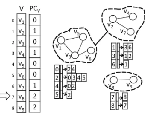
As an example, let Geβ be initially empty and D = {d1, d2, . . . , d9}be the set of documents that will be added to the collection. For the sake of simplicity, we will assume that CUDA-DClus already added the documents inGeβ as
vertices and that the similarities existing between each pair of documents are those showed in Table 1. Taking into ac-count the above mentioned information, Figures 9, 10, 11 and 12 exemplify how CUDA-DClus builds the array of partial connected components representing graph Geβ, for β = 0.3.
Vert./Vert. v1 v2 v3 v4 v5 v6 v7 v8 v9
v1 - 0 0.4 0 0.5 0 0 0 0
v2 0 - 0 0.4 0 0 0.5 0 0
v3 0.4 0 - 0.7 0.6 0.3 0 0 0
v4 0 0 0.7 - 0 0 0 0 0
v5 0.5 0 0.6 0 - 0 0 0 0
v6 0 0 0.3 0 0 - 0 0 0
v7 0 0 0 0 0 0 - 0 0
v8 0 0 0 0 0 0 0 - 0.5
v9 0 0 0 0 0 0 0 0.5
-Table 1: Similarities existing between each pair of vertices of the example.
V
v1
v2
v3
v4
v5
v6
v 7
v 8
v 9
PC V
0
-1
0
-1
0
-1
-1
-1
-1 0
1
2
3
4
5
6
7
8
v 1
v5
v3
0
2
4 2 4
0
0
Figure 9: Processing vertexv1.
V
v1 v2 v3 v4 v5 v6 v7 v8 v9
PCV 0
1
0
1
0
-1
1
-1
-1 0 1 2 3 4 5 6 7 8
v2 v4
v7
1
3
6 3 6
1
1
v1 v5
v3
0
2
4 2 4
0
0
Figure 10: Processing vertexv2.
from Figure 11, when vertexv3is being processed, CUDA-DClus updates the first PCC by adding vertexv6and upda-ting the adjacency list of verticesv3andv5; CUDA-DClus also updates the second PCC by modifying the adjacency list of vertexv4, which is similar to vertexv3. In this exam-ple, these two partial connected components were joined by a dash line in order to illustrate the fact that they are linked since vertices v3, belonging to the first PCC, andv4, be-longing to the second PCC, are similar. Finally, the third PCC is created when CUDA-DClus processes vertex v8,
V
v1 v2 v3 v4 v5 v6 v7 v8 v9
PCV 0
1
0
1
0
0
1
-1
-1 0 1 2 3 4 5 6 7 8
v1 v5
v3
v2 v4
v7
v6
0
2
4
5 2 4
0 3 4 5
0 2
1
3
6 3 6
1 1 2
2
Figure 11: Processing vertexv3.
V v1 v2 v3 v4 v5 v6 v7 v8 v9
PCV 0 1 0 1 0 0 1 2 2 0
1
2
3
4
5
6
7
8
v1 v5
v3
v2 v4
v7
v6
v8 v9 7
8 8
7 0
2
4
5 2 4
0 3 4 5
0 2
2
1
3
6 3 6
1 1 2
Figure 12: Processing vertexv8.
as it can be seen in Figure 12. The processing of vertices
v4, v5, v6, v7 andv9 does not affect the partial connected components built so far, therefore, it was not included in the example.
We would like to emphasize two facts about the above commented process. The first fact is that, since this is the first time the array ArrP CC representingGeβ is built, all
these components are already in system memory. The se-cond fact is that if we put a PPC Pi ∈ ArrP CC into a
setQPi and then, iteratively we add toQPi all the linked
PCC of each PCC belonging to QPi, the resulting set is
a connected component. Proof is straightforward by con-struction. Hereinafter, we will say that QPi is the
con-nected component induced by PCCPi.
Once the array ArrP CC representing Geβ was built,
CUDA-DClus processes each of its partial connected com-ponents in order to build the clustering. For processing a PCC Pi ∈ ArrP CC that has not been processed in a
previous iteration, CUDA-DClus first buildsQPiand then,
be-longing to this component using the strategy proposed by CUDA-OClus. Once the relevance of the vertices have been recomputed, CUDA-DClus follows the same steps used by DClustR for updating the covering and conse-quently, the clustering ofQPi. Remaining steps of DClustR
were not implemented in CUDA because they are more fa-vored with a CPU implementation. Once the clustering has been updated, CUDA-DClus stores the existing partial con-nected components in the hard drive, releasing in this way the system memory.
OnceGeβ changes due to the additions of documents to
the collection, CUDA-DClus updates the array ArrP CC
representing Geβ and then, it updates the current
cluste-ring. In order to update the arrayArrP CC, CUDA-DClus
adds for each incoming document, a vertex in Geβ and
then, CUDA-DClus sets to -1 the entries that these verti-ces occupy in P CV, in order to express that they do not
belong to any PCC yet. LetM ={v1, v2, . . . , vk}be the
set of added vertices. Afterwards, for processing a ver-texvi ∈M, CUDA-DClus slightly modifies the strategy it
uses for creating the partial connected components. Now, rather than computing the similarity ofvionly with the
ver-tices that came aftervi inV (i.e., Sucvi), CUDA-DClus
also computes the similarity ofvi with respect to the
ver-tices that belong toGeβ before the changes; that is, the
si-milarities are now computed betweenviand each vertex in Sucvi∪(V \M). Remaining steps are the same.
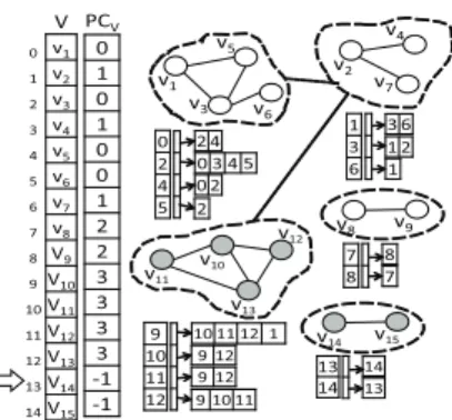
LetD1 = {d10, d11, . . . , d15} be the set of documents that were added to the collection represented by graphGeβ,
whose array of partial connected components was built in Figure 9, and letv10, v11, . . . , v15be the vertices that were consequently added inGeβby CUDA-DClus. For the sake
of simplicity, in the example it is assumed that none of the vertices belonging toGeβ before the changes is similar to
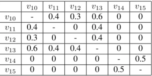
the added vertices, with the only exception of v2 whose similarity with v10 is0.5. Table 2 shows the similarities between each pair of the added vertices. Figures 13, 14, 15 and 16 show, assumingβ = 0.3, how CUDA-DClus upda-tes the array of partial connected components representing
e
Gβ after the above mentioned additions. In these figures,
vertices filled with light gray are those that were added to the collection.
v10 v11 v12 v13 v14 v15
v10 - 0.4 0.3 0.6 0 0
v11 0.4 - 0 0.4 0 0
v12 0.3 0 - 0.4 0 0
v13 0.6 0.4 0.4 - 0 0
v14 0 0 0 0 - 0.5
v15 0 0 0 0 0.5
-Table 2: Similarities existing between each pair of added vertices.
As it can be seen in Figure 13, firstly, CUDA-DClus pro-cesses vertexv10and, as a result of this processing, another PCC is created for containing verticesv10, v11, v12andv13. This new PCC was joined with the PCC determined by
ver-V v 1 v 2 v 3 v 4 v 5 v6 v 7 v8 V 9 V 10 V 11 V 12 V13 V 14 V15 PC V 0 1 0 1 0 0 1 2 2 3 3 3 3 -1 -1 0 1 2 3 4 5 6 7 8 9 10 11 12 13 14 v1 v5 v3 v2 v4 v7 v6
v8 v9 7 8 8 7 0 2 4 5 2 4
0 3 4 5
0 2 2 1 3 6 3 6 1 1 2 v10 v12 v11 v13 9 10 11 12 9 10 11 12 1
9
9
Figure 13: Processing vertexv10.
V v 1 v 2 v 3 v4 v 5 v6 v 7 v 8 V 9 V 10 V11 V 12 V13 V 14 V 15 PCV 0 1 0 1 0 0 1 2 2 3 3 3 3 -1 -1 0 1 2 3 4 5 6 7 8 9 10 11 12 13 14 v1 v5 v3 v2 v4 v7 v6
v8 v9 7 8 8 7 0 2 4 5 2 4
0 3 4 5
0 2 2 1 3 6 3 6 1 1 2 v10 v12 v11 v13 9 10 11 12 9 12 10 11 12 1
9
9 10
Figure 14: Processing vertexv11.
V v 1 v2 v 3 v4 v 5 v 6 v 7 v 8 V9 V 10 V11 V 12 V 13 V 14 V 15 PCV 0 1 0 1 0 0 1 2 2 3 3 3 3 -1 -1 0 1 2 3 4 5 6 7 8 9 10 11 12 13 14 v1 v5 v3 v2 v4 v7 v6
v8 v9 7 8 8 7 0 2 4 5 2 4
0 3 4 5
0 2 2 1 3 6 3 6 1 1 2 v10 v12 v11 v13 9 10 11 12 9 12 10 11 12 1
9 12
9 10 11
Figure 15: Processing vertexv12.
V v
1
v
2
v
3
v
4
v
5
v6
v
7
v8
V
9
V
10
V
11
V
12
V13
V
14
V15
PC
V
0 1 0 1 0 0 1 2 2 3 3 3 3 -1 -1
0
1
2
3
4
5
6
7
8
9
10
11
12
13
14
v1
v5
v3
v2
v4
v7
v6
v8 v9 7
8 8
7 0
2
4
5 2 4
0 3 4 5
0 2
2
1
3
6 3 6
1 1 2
v10
v12
v11
v13 9
10
11
12 9 12 10 11 12 1
9 12
9 10 11
v14 v15 13
14 14
13
Figure 16: Processing vertexv14.
see Figure 16; this PCC contains verticesv14andv15. Once the array ArrP CC has been updated,
CUDA-DClus processes each new PCC following the same stra-tegy commented above, in order to update the current clus-tering. It is important to highlight that, different from when
ArrP CC was created, this time the partial connected
com-ponents loaded into the system memory are those belon-ging to the connected components determined by each new created PCC; the other partial connected components re-main in the hard drive. Although in the worst scenario an incoming document can be similar to all existing docu-ments in the collection, generally similarity graphs are very sparse so it is expected that the new representation pro-posed by CUDA-DClus as well as the strategy it uses for updating the array of partial connected components, help CUDA-DClus to save system memory.
4
Experimental results
In this section, the results of several experiments done in order to show the performance of the CUDA-OClus and CUDA-DClus algorithms are presented. The experiments were conducted over eight document collections and were focused on: (1) assessing the correctness of the proposed parallel algorithms wrt. their original non parallel versi-ons, (2) evaluating the improvement achieved by the pro-posed algorithms with respect to the original OClustR and DClustR algorithms, and (3) evaluating the memory both CUDA-DClus and DClustR consume when they are pro-cessing the same collection. All the algorithms were imple-mented in C++; the codes of OClustR and DClustR algo-rithms were obtained from their authors. For implementing CUDA-OClus and CUDA-DClus the CUDA Toolkit 5.5 was used. All the experiments were performed on a PC with Core i7-4770 processor at 3.40 GHz, 8GB RAM, ha-ving a PCI express NVIDA GeForce GT 635, with 1 GB DRAM.
The document collections used in our experiments were built from two benchmark text collections
com-monly used in documents clustering: Reuters-v2 and TDT2. The Reuters-v2 can be obtained from http://kdd.ics.uci.edu, while TDT2 benchmark can be obtained from http://www.nist.gov/speech/tests/tdt.html. From these benchmarks, eight document collections were built. The characteristics of these collections are shown in Table 3. As it can be seen from Table 3, these collections are heterogeneous in terms of their size, dimension and the average size of the documents they contain.
Coll. #Docs. #Terms Terms/Docs. Reu-10K 10000 33370 27 Reu-20K 20000 48493 41 Reu-30K 30000 59413 50 Reu-40K 40000 70348 58 Reu-50K 50000 74720 64 Reu-60K 60000 81632 69 Reu-70K 70000 91490 76 Tdt-65K 65945 114828 210
Table 3: Overview of the collections used in our experi-ments.
In our experiments, documents were represented using the Vector Space Model (VSM) [13]. The index terms of the documents represent the lemmas of the words occurring at least once in the collection; these lemmas were extracted from the documents using Tree-tagger1. Stop words such as: articles, prepositions and adverbs were removed. The index terms of each document were statistically weighted using their term frequency. Finally, the cosine measure was used to compute the similarity between two documents [9].
4.1
Correctness evaluation
As it was mentioned before, the first experiment was fo-cused on assessing the correctness of the proposed algo-rithms. With this aim, we will compare the clusterings built by CUDA-OClus and CUDA-DClus with respect to those built by the original OClustR and DClustR algorithms, un-der the same conditions. For evaluating CUDA-OClus we selected the Reu-10K, Reu-20K, Reu-30K, Reu-40K and Reu-50K collections; whilst for evaluating CUDA-DClus we selected Reu-10K, Reu-20K and Reu-30K collections. These collections were selected due to they resemble the collections over which both OClustR and DClustR were evaluated in [6] and [7], respectively.
In order to evaluate CUDA-OClus, we executed OClustR and CUDA-OClus over the Reu-10K, Reu-20K, Reu-30K, Reu-40K and Reu-50K collections, using β = 0.25 and
0.35. We used these threshold values as these values obtai-ned the best results in several collections as reported in the original OClustR [6] and DClustR [7] articles. Then, we took the clustering results obtained by OClustR asground truthand we evaluateds the clustering results obtained by CUDA-OClus in terms of their accuracy, using the
bed [14] and the Normalized Mutual Information (NMI) [15] external evaluation measures.
FBcubed is one of the external evaluation measures most used for evaluating overlapping clustering algorithms and unlike of other external evaluation metrics, it meets with four fundamental constrains proposed in [14] (cluster ho-mogeneity, cluster completeness, rag bag and cluster size vs quantity). On the other hand, NMI is a measure of si-milarity borrowed from information theory, which has pro-ved to be reliable [15]. Both metrics take values in [0,1], where1means identical results and0completely different results. In order to take into account the inherent data order dependency of CUDA-OClus, we executed CUDA-OClus twenty more times over the above mentioned collections, for each parameter value, varying the order of their docu-ments. Table 4 shows the average FBcubed and NMI va-lues attained by CUDA-OClus for each selected collection, usingβ = 0.25and0.35.
FBCubed
ThresholdReu-10K Reu-20K Reu-30K Reu-40K Reu-50K
β=0.25 0.999 0.999 1.000 0.998 1.000 β=0.35 0.999 1.000 1.000 1.000 0.999
NMI
ThresholdReu-10K Reu-20K Reu-30K Reu-40K Reu-50K
β=0.25 0.997 0.999 1.000 0.999 1.000 β=0.35 0.998 1.000 1.000 1.000 0.999
Table 4: Average FBcubed and NMI values attained by CUDA-OClus for each selected collection.
As it can be seen from Table 4, the average FBcubed and NMI values attained by CUDA-OClus are very close to 1, meaning that the clusters CUDA-OClus builds are al-most identical to those built by OClustR. The differences between the clusterings are caused by the inherent data or-der dependency of the algorithms and also because of the different floating point arithmetic used by CUDA.
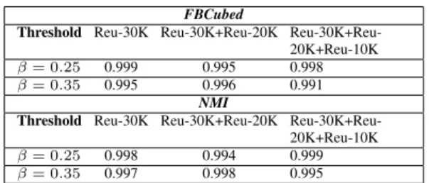
In order to asses the validity of CUDA-DClus, in the se-cond part of the first experiment, we will compare the clus-tering results built by CUDA-DClus with respect to those obtained by DClustR. With this aim, we obtain a ground truth by executing DClustR over the Reu-30K collection, also using β = 0.25 and β = 0.35, and then, we pro-cess Reu-20K and Reu-10K collections, in this order, as if they were additions of documents to the collection. That is, we are going to add the documents contained in Reu-20K to the current collection (i.e., Reu-30K) and update the clustering using DClustR and after that, we are goind to add Reu-10K to the collection resulting from previous additions (i.e., Reu-30K union Reu-20K) and update the clustering again. We repeated the above mentioned exe-cution under the same parameter configuration but using CUDA-DClus instead of DClustR and afterwards. Then, we take the results obtained by DClustR as ground truth and we evaluate each of the three clustering results obtai-ned by CUDA-DClus in terms of their accuracy, using the FBcubed and NMI external evaluation measures. Like in the first part of this experiment, we executed CUDA-DClus twenty times under the above mentioned experimental
con-figuration, each time varying the order of the documents inside the collections. Table 5 shows the average FBcu-bed and NMI values attained by CUDA-DClus for each se-lected collection, usingβ = 0.25and0.35.
FBCubed
Threshold Reu-30K 20K
Reu-30K+Reu-20K+Reu-10K
β= 0.25 0.999 0.995 0.998
β= 0.35 0.995 0.996 0.991
NMI
Threshold Reu-30K 20K
Reu-30K+Reu-20K+Reu-10K
β= 0.25 0.998 0.994 0.999
β= 0.35 0.997 0.998 0.995
Table 5: Average FBcubed and NMI values attained by CUDA-DClus for each selected collection.
As it can be seen from Table 5, the average FBcubed and NMI values attained by CUDA-DClus are very close to 1, meaning that the clusters it builds are almost identical to those built by DClustR. From this first experiment, we can conclude that the speed-up attained by CUDA-OClus and CUDA-DClus does not degrade their accuracy wrt. the original non parallel versions.
4.2
Execution time evaluation
In the second experiment, we evaluate the time impro-vement achieved by CUDA-OClus and CUDA-DClus with respect to OClusR and DClustR, respectively. With this aim, we execute both OClustR and CUDA-OClus over 10K, 20K, 30K, 40K, 50K, Reu-60K and Reu-70K, usingβ = 0.25and0.35and we mea-sured the time they spent. Like in the previous experiment, in order to take into account the data order dependency of both algorithms, we repeated the above mentioned execu-tions twenty times, for each collection and each parame-ter configuration, but varying the order of the documents of the collections. Figure 17 shows the average time both OClustR and CUDA-OClus spent for clustering each se-lected collection, for each parameter configuration.
0 257 514 771 1028
Reu-10K Reu-20K Reu-30K Reu-40K Reu-50K Reu-60K Reu-70K
T
im
e
(
se
c.
)
Collec!ons OClustR
CUDA-Clus
(a)β= 0.25
0 215 430 645 860
Reu-10K Reu-20K Reu-30K Reu-40K Reu-50K Reu-60K Reu-70K
T
im
e
(
se
c.
)
Collec!ons OClustR
CUDA-Clus
(b)β= 0.35
Figure 17: Time spent by OClustR and CUDA-OClus for clustering the selected experimental datasets, using β = 0.25and0.35.
task over a specific block, then we expect that if we use a powerful GPU with more streaming multiprocessor, the difference between the processing time achieved by paral-lel version and sequential version will be higher than the one showed in this experiments.
In order to compare both DClustR and CUDA-DClus, in the second part of the second experiment, we clustered the Reu-50K collection using both algorithms and then, we measured the time each algorithm spent for updating the current clustering each timeN documents of Tdt-65K col-lection are incrementally added to the existing colcol-lection. In this experiment we also usedβ = 0.25and0.35, and we setN = 5000 andN = 1000which are much grea-ter values than those used to evaluate DClustR [7]. In or-der to take into account the data oror-der dependency of both algorithms, the above mentioned executions were also re-peated twenty times, for each collection and each parame-ter configuration, but varying the order of the documents of the collections. Figure 18 shows the average time both DClustR and CUDA-DClus spent for updating the current clustering, for each parameter configuration.
As it can be seen from Figure 18, CUDA-DClus has a better behavior than DClustR, for each parameter
configu-0 200 400 600
5 10 15 20 25
T
im
e
(
se
c.
)
Objects (1*103) DClustR
CUDA-DClus
(a)β= 0.25,N= 5000
0 150 300 450 600
5 10 15 20 25
T
im
e
(
se
c.
)
Objects (1*103)
DClustR
CUDA-DClus
(b)β= 0.35,N= 5000
0 350 700 1050 1400
10 20 30 40 50
T
im
e
(
se
c.
)
Objects (1*103)
DClustR
CUDA-DClus
(c)β= 0.25,N= 10000
0 350 700 1050 1400
10 20 30 40 50
T
im
e
(
se
c.
)
Objects (1*103) DClustR
CUDA-DClus
(d)β= 0.35,N= 10000
Figure 18: Time spent by DClustR and CUDA-DClus for updating the current clustering, usingβ = 0.25and0.35, forN = 5000and10000.
ration, when multiple additions are processed over the se-lected dataset, showing an average speed up of 1.25x and 1.29x forβ = 0.25, N = 5000andβ = 0.35, N = 5000
β = 0.35, N = 10000respectively. As in the first part of this experiment, it can be seen also from Figure 18, that the behavior of CUDA-DClus, with respect to that of DClustR, becomes better as the size of the collection grows; in this way, we can say that CUDA-DClus also scales well as the size of the collection grows.
4.3
Memory use evaluation
Although the spatial complexity of both algorithm is
O(|V|+ Eeβ
), the strategy CUDA-DClus proposes for
re-presenting Geβ should allow to reduce the amount of
me-mory needed to update the clustering each time the col-lection changes. Thus, in the third experiment, we compare the amount of memory used by CUDA-DClus against that used by DClustR, when processing the changes performed in the second experiment. The amount of connected com-ponent loaded by both algorithms when they are updating the current clustering after changes, is directly proportio-nal to the memory used. Based on this, Figure 19 shows the average number of connected components (i.e., Ave. NCC) each algorithm load into system memory, when processing the changes presented in Figure 18, for each parameter con-figuration.
As it can be seen from Figure 19, CUDA-DClus consu-mes less memory than DClustR, for each parameter con-figuration, thereby hence resulting the memory usage of CUDA-DClus is respectively 22.43% for β = 0.25and
42.46% forβ = 0.35less than the one of DClustR. The above mentioned characteristic, plus the fact that CUDA-DClus is also faster than CUDA-DClustR, makes CUDA-CUDA-DClus suitable for applications processing large document col-lections.
We would like to highlight that in the worst scenario, if the clustering of all the connected components needs to be updated, all the partial connected components will be loaded to system memory and thus, our proposed CUDA-DClus and CUDA-DClustR will have a similar behavior. Addi-tionally, taking into account the results of experiments in sections 4.1 and 4.2, we can conclude that the strategy pro-posed for reducing the memory used by CUDA-DClus does not include any considerable cost in the overall processing time of CUDA-DClus or in its accuracy.
5
Conclusions
In this paper, we introduced two GPU-based parallel versi-ons of the OClustR and DClustR clustering algorithms, na-mely CUDA-OClus and CUDA-DClus, specifically tailo-red for document clustering. CUDA-OClus proposes a stra-tegy in order to speed up the most time consuming steps of OClustR. This strategy is reused by CUDA-DClus in or-der to speed up the most time consuming steps of DClustR. Moreover, CUDA-DClus proposes a new strategy for re-presenting the graph Geβ that DClustR uses for
represen-ting the collection of documents. This new representation
60 100 140 180
5 10 15 20 25
A
v
e
.
N
C
C
Objects (1*103) DClustR
CUDA-DClus
(a)β= 0.25,N= 5000
500 900 1300 1700 2100 2500
5 10 15 20 25
A
v
e
.
N
C
C
Objects (1*103) DClustR
CUDA-DClus
(b)β= 0.35,N= 5000
100 140 180 220
10 20 30 40 50
A
v
e
.
N
C
C
Objects (1*103) DClustR
CUDA-DClus
(c)β= 0.25,N= 10000
500 1500 2500 3500
10 20 30 40 50
A
v
e
.
N
C
C
Objects (1*103) DClustR
CUDA-DClus
(d)β= 0.35,N= 10000
Figure 19: Average number of connected components DClustR and CUDA-DClus load into system memory when they are updating the current clustering, usingβ = 0.25and0.35, forN = 5000and10000.
with no extra cost.
The proposed parallel algorithms were compared against their original versions, over several standard document collections. The experiments were focused on: (a) as-sess the correctness of the proposed parallel algorithms, (b) evaluate the speed-up achieved by CUDA-OClus and CUDA-DClus with respect to OClustR and DClustR, re-spectively, and (c) evaluate the memory both CUDA-DClus and DClusR consumes when they are processing changes. From the experiments, it can be seen that both CUDA-OClus and CUDA-DClus are faster than CUDA-OClustR and DClustR, respectively, and that the speed up these parallel versions attain do not degrade their accuracy. The experi-ments also showed that CUDA-DClus consumes less me-mory than DClustR, when both algorithms are processing changes over the same collection.
Based on the obtained results, we can conclude that both CUDA-OClus and CUDA-DClus enhance the efficiency of OClustR and DClustR, respectively, in problems dealing with a very large number of documents. These parallel al-gorithms could be useful in applications, like for instance news analysis, information organization and profiles iden-tification, among others. We would like to mention, that even when the proposed parallel algorithms were specifi-cally tailored for processing documents with the purpose of using the cosine measure, the strategy they propose can be easily extended to work with other similarity or distance measures like, for instance, euclidean and manhattan dis-tances.
As future work, we are going to explore the use in CUDA-OClus and CUDA-DClus of other types of memo-ries in GPU such as texture memory, which is a faster me-mory than the one both CUDA-OClus and CUDA-DClus are using now. Besides, we are going to evaluate both al-gorithms over more faster GPU cards, in order to have a better insight of the performance of both algorithms when the number of CUDA cores are increased.
References
[1] E. Bae, J. Bailey, G. Dong, A clustering comparison measure using density profiles and its application to the discovery of alternate clusterings, Data Mining and Knowledge Discovery 21 (3) (2010) 427–471.
[2] A. K. Jain, M. N. Murty, P. J. Flynn, Data clustering: a review, ACM computing surveys (CSUR) 31 (3) (1999) 264–323.
[3] S. Gregory, A fast algorithm to find overlapping com-munities in networks, in: Machine learning and kno-wledge discovery in databases, Springer, 2008, pp. 408–423.
[4] J. Aslam, K. Pelekhov, D. Rus, Static and dynamic in-formation organization with star clusters, in: Procee-dings of the seventh international conference on
In-formation and knowledge management, ACM, 1998, pp. 208–217.
[5] A. Pons-Porrata, R. Berlanga-Llavori, J. Ruiz-Shulcloper, J. M. Pérez-Martínez, Jerartop: A new topic detection system, in: Progress in Pattern Re-cognition, Image Analysis and Applications, Sprin-ger, 2004, pp. 446–453.
[6] A. Pérez-Suárez, J. F. Martínez-Trinidad, J. A. Carrasco-Ochoa, J. E. Medina-Pagola, Oclustr: A new graph-based algorithm for overlapping cluste-ring, Neurocomputing 121 (2013) 234–247.
[7] A. Pérez-Suárez, J. F. Martínez-Trinidad, J. A. Carrasco-Ochoa, J. E. Medina-Pagola, An algo-rithm based on density and compactness for dynamic overlapping clustering, Pattern Recognition 46 (11) (2013) 3040–3055.
[8] L. J. G. Soler, A. P. Suárez, L. Chang, Efficient over-lapping document clustering using gpus and multi-core systems, in: Progress in Pattern Recognition, Image Analysis, Computer Vision, and Applications - 19th Iberoamerican Congress, CIARP 2014, Puerto Vallarta, Mexico, November 2-5, 2014. Proceedings, 2014, pp. 264–271.
[9] M. W. Berry, M. Castellanos, Survey of text mining, Computing Reviews 45 (9) (2004) 548.
[10] R. Gil-García, A. Pons-Porrata, Dynamic hierarchical algorithms for document clustering, Pattern Recogni-tion Letters 31 (6) (2010) 469–477.
[11] J. Sanders, E. Kandrot, CUDA by example: an introduction to general-purpose GPU programming, Addison-Wesley Professional, 2010.
[12] D. B. Kirk, W. H. Wen-mei, Programming massively parallel processors: a hands-on approach, Newnes, 2012.
[13] G. Salton, A. Wong, C.-S. Yang, A vector space mo-del for automatic indexing, Communications of the ACM 18 (11) (1975) 613–620.
[14] E. Amigó, J. Gonzalo, J. Artiles, F. Verdejo, A com-parison of extrinsic clustering evaluation metrics ba-sed on formal constraints, Information retrieval 12 (4) (2009) 461–486.