Forecast covariances in the linear multiregression dynamic
model.
Catriona M Queen, Ben J Wright and Casper J Albers The Open University, Milton Keynes, MK7 6AA, UK
February 28, 2007 Abstract
The linear multiregression dynamic model (LMDM) is a Bayesian dynamic model which preserves any conditional independence and causal structure across a multivariate time series. The conditional independence structure is used to model the multivariate series by separate (conditional) univariate dynamic lin-ear models, where each series has contemporaneous variables as regressors in its model. Calculating the forecast covariance matrix (which is required for calculating forecast variances in the LMDM) is not always straightforward in its current formulation. In this paper we introduce a simple algebraic form for calculating LMDM forecast covariances. Calculation of the covariance be-tween model regression components can also be useful and we shall present a simple algebraic method for calculating these component covariances. In the LMDM formulation, certain pairs of series are constrained to have zero forecast covariance. We shall also introduce a possible method to relax this restriction. Keywords: Multivariate time series, dynamic linear model, conditional inde-pendence, forecast covariance matrix, component covariances
1
Introduction.
A multiregression dynamic model (MDM) (Queen and Smith, 1993) is a non-Gaussian multivariate state space time series model. The MDM has been designed for forecasting time series for which, at any one time period, a conditional independence structure across the time series and causal drive through the system can be hypothesized. Such series can be represented by a directed acyclic graph (DAG) which, in addition to giving a useful pictorial representation of the structure of the multivariate series, is used to decompose the multivariate time series model into simpler (conditional) univariate dynamic models (West and Harrison, 1997). As such, the MDM is a graphical model (see, for example, Cowell et al. (1999)) for multivariate time series, which simplifies computation in the model through local computation. Like simultaneous equation models, in the MDM each univariate series has contemporaneous variables as regressors in its model. When these
regressions are linear, we have a linear MDM (LMDM) and in this case we have a set of univariate regression dynamic linear models (DLM’s) (West and Harrison, 1997, Section 9.2). Like a non time series graphical model, the conditional univariate models in an MDM are computationally simple to work with (in this case univariate DLM’s), while the joint distribution can be arbitrarily complex. Also, because the model is a collection of uni-variate dynamic models, the MDM avoids the difficult problem of eliciting an observation covariance matrix for the multivariate problem. It also avoids the alternative of learn-ing about the covariance matrix on-line via the matrix normal DLM (West and Harrison (1997), Section 16.4) whose use is restricted to problems in which all the individual series are similar.
Many multivariate time series may be suitable for use with an LMDM. For example, Queen (1994) uses the LMDM to model monthly brand sales in a competitive market. In this application, the competition in the market is the causal drive within the system and is used to define a conditional independence structure across the time series. Queen (1997) and Queen et al. (1994) focus on how DAG’s may be elicited for market models. DAG’s are also used to represent brand relationships when forecasting time series of brand sales in Goldstein et al. (1993), Farrowet al. (1997) and Farrow (2003). As another example, Whitlock and Queen (2000) and Queen et al. (2007) use the LMDM to model hourly vehicle counts at various points in a traffic network. Here, as in Sun et al. (2006), the direction of traffic flow produces the causal drive in the system and the possible routes through the network are used to define a conditional independence structure across the time series. The LMDM then produces a set of regression DLM’s where contemporaneous traffic flows at upstream links in the network are used as linear regressors. Tebaldi et al.
(2002) also use regression DLM’s when modelling traffic flows. Like Queen et al. (2007), they use traffic flows at upstream links in the network as linear regressors. However, whereas the vehicle counts in Queen et al. (2007) are for one-hour intervals, those in Tebaldiet al. (2002) are for one-minute intervals, and so regression on lagged flows (rather than contemporaneous flows) is required. Fosen et al. (2006) use similar ideas to the LMDM when proposing a dynamical graphical model combining the additive hazard model and classical path analysis to analyse a trial of cancer patients with liver cirrhosis. Like the LMDM, their model uses linear regression with parents from the DAG as regressors. The focus, however, is to investigate the treatment effects on the variates over time, rather than forecasts of the variables directly.
There are many other potential application areas for the LMDM, including problems in economics (modelling various economic indicators such as energy consumption and GDP), environmental problems (such as water and other resource management problems), industrial problems (such as product distribution flow problems) and medical problems (such as patient physiological monitoring).
When using the LMDM it is important to be able to calculate the forecast covariance matrix for the series. Not only is this of interest in its own right, it is also required for calculating the forecast variances for the individual series. Queen and Smith (1993) presented a recursive form for the covariance matrix, but this is not in an algebraic form which is always simple to use in practice. In this paper we introduce a simple algebraic method for calculating forecast covariances in the LMDM.
Following the superposition principle (see West and Harrison (1997), p98), each con-ditional univariate DLM in an LMDM can be thought of as the sum of individual model components. For example, a DLM may have a trend component, a regression component, and so on. In an LMDM it can be useful to calculate the covariance between individual DLM regression components for different series and here we introduce a simple algebraic method for calculating such component covariances.
The paper is structured as follows. In the next section the LMDM is described and its use is illustrated using a bivariate time series of brand sales. Section 3 presents a simple algebraic method for calculating the LMDM one-step andk-step ahead forecast covariance matrices. Component covariances are introduced in Section 4, along with a simple method to calculate them. In the LMDM formulation, certain pairs of series are constrained to have zero forecast covariance and Section 5 introduces a possible method to relax this restriction. Finally, Section 6 gives some concluding remarks.
2
The Linear Multiregression Dynamic Model
We have a multivariate time series Yt = (Yt(1), . . . , Yt(n))T. Suppose that the series is ordered and that the same conditional independence and causal structure is defined across the series through time, so that at each time t= 1,2, . . ., we have
Yt(r)∐ {{Yt(1), . . . , Yt(r−1)} \pa(Yt(r))} |pa(Yt(r)) forr= 2, . . . n
which reads “Yt(r) is independent of {Yt(1), . . . , Yt(r−1)} \pa(Yt(r)) given pa(Yt(r))”
Each variable in the set pa(Yt(r)) is called aparent ofYt(r) and Yt(r) is known as achild
of each variable in the set pa(Yt(r)). We shall call any series for which pa(Yt(·)) =∅, a
root node and list all root nodes before any children in the ordered seriesYt.
The conditional independence relationships at each time point t can be represented by a DAG, where there is a directed arc to Yt(r) from each of its parents in pa(Yt(r)).
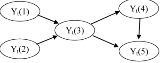
To illustrate, Figure 1 shows a DAG for five time series at time t, where pa(Yt(2)) = ∅,
pa(Yt(3)) ={Yt(1), Yt(2)}, pa(Yt(4)) ={Yt(3)} and pa(Yt(5)) ={Yt(3), Yt(4)}. Note that
both Yt(1) andYt(2) are root nodes.
Figure 1: DAG representing five time series at timet.
Suppose further that there is a conditional independence and causal structure defined for the processes so that, ifYt(r) = (Y1(r), . . . , Yt(r))T,
Yt(r)∐
©©
Yt(1), . . . ,Yt(r−1)ª
\pa(Yt(r))ª
|pa(Yt(r)),Yt−1(r) forr= 2, . . . n. Denote the information available at time t by Dt. An LMDM has the following system
equation and nobservation equations for all times t= 1,2, . . ..
Observation equations: Yt(r) = Ft(r)Tθt(r) +vt(r), vt(r)∼N(0, Vt(r)) 1≤r≤n
System equation: θt = Gtθt−1+wt, wt∼N(0, Wt) Initial Information: (θ0|D0) ∼ N(m0, C0).
The vector Ft(r) contains the parents pa(Yt(r)) and possibly other known variables (which may include Yt−1(r) and pa(Yt−1(r))); θt(r) is the parameter vector for Yt(r);
Vt(1), . . . Vt(n) are the scalar observation variances; θTt = (θt(1)T, . . . ,θt(n)T); and the
matrices Gt, Wt and C0 are all block diagonal. The error vectors, vTt={vt(1), . . . , vt(n)}
and wT t=
©
wt(1)T, . . . ,w t(n)T
ª
, are such that vt(1), . . . , vt(n) and wt(1), . . . ,wt(n) are
mutually independent and {vt,wt}t≥1 are mutually independent with time.
The LMDM therefore uses the conditional independence structure to model the mul-tivariate time series by n separate univariate models — for Yt(1) and Yt(r)|pa(Yt(r)),
r = 2, . . . , n. For those series with parents, each univariate model is simply a regression DLM with the parents as linear regressors. For root nodes, any suitable univariate DLM may be used. For example, consider the DAG in Figure 1. AsYt(1) andYt(2) are both root
nodes, each of these series can be modelled separately in an LMDM using any suitable uni-variate DLMs. Yt(3), Yt(4) andYt(5) all have parents and so these would be modelled by
(separate) univariate regression DLMs with the two regressors Yt(1) andYt(2) forYt(3)’s
model, the single regressor Yt(3) forYt(4)’s model and the two regressorsYt(3) andYt(4)
forYt(5)’s model.
As long asθt(1),θt(2), . . . ,θt(n) are mutually independent a priori, eachθt(r) can be updated separately in closed form fromYt(r)’s (conditional) univariate model. A forecast
forYt(1) and the conditional forecasts forYt(r)|pa(Yt(r)),r = 2, . . . , n, can also be found
separately using established DLM results (see West and Harrison (1997) for details). For example, in the context of the DAG in Figure 1, forecasts can be found separately (using established DLM results) for
Yt(1), Yt(2), Yt(3)|Yt(1), Yt(2), Yt(4)|Yt(3) and Yt(5)|Yt(3), Yt(4).
However, Yt(r) and pa(Yt(r)) are observed simultaneously. So the marginal forecast for
each Yt(r), without conditioning on the values of its parents, is required. Unfortunately,
the marginal forecast distributions forYt(r),r = 2, . . . , n, will not generally be of a simple
form. However, (under quadratic loss), the mean and variance of the marginal forecast distributions for Yt(r), r = 2, . . . , n, are adequate for forecasting purposes, and these can
be calculated. So, returning to the context of the DAG in Figure 1, this means that the marginal forecast means and variances for Yt(3), Yt(4) and Yt(5) need to be calculated.
Note that asYt(1) andYt(2) do not have any parents, their marginal forecasts have already
been calculated from DLM theory.
For calculating the marginal forecast variance for Yt(r), the marginal forecast
covari-ance matrix for pa(Yt(r)) is required. Returning to the example DAG in Figure 1 to
illustrate, this means that the marginal forecast variance of Yt(5), for example, requires
the forecast covariance forYt(3) andYt(4), without conditioning on either of their parents
Yt(1) and Yt(2) — that is, the marginal covariance ofYt(3) and Yt(4). The marginal
fore-cast covariance matrix also provides information about the structure of the multivariate series, and, as such, is of interest in its own right. Queen and Smith (1993) gave a recursive form for calculating the marginal forecast covariance matrix. However, this is not always
easy to use in practice. Section 3 presents a simple algebraic form for calculating marginal forecast covariances. First, we shall illustrate how the LMDM works in practice.
2.1 Example: forecasting a bivariate time series of brand sales
We shall illustrate using a simple LMDM for a bivariate series of monthly brand sales. The series consist of 34 months of data (supplied by Unilever Research) for two brands, which we shall call B1 and B2, who compete with each other in a product market.
Denote the sales at each timetfor brands B1 and B2 byXt(1) andXt(2), respectively.
LetYtbe the total number of sales of B1 and B2 in montht(so thatYt=Xt(1) +Xt(2)).
Then Yt can be modelled by a Poisson distribution with some mean µt, denoted P o(µt).
Suppose that for each individual purchase of this product in month t,
P(B1 purchased|B1 or B2 purchased) =θt.
Then, Xt(1), the number of B1 purchased in month t, can be modelled by a binomial
distribution with sample size Yt, the total number of B1 and B2 purchased in month t,
and parameterθt — that is,Xt(1)|Yt∼Bi(Yt, θt).
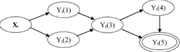
These distributions forYtandXt(1) can be represented by the DAG in Figure 2. Xt(2)
is a logical function of its parents and is known once its parents are known. Following the terminology of WinBUGS software (http://www.mrc-bsu.cam.ac.uk/bugs/) we shall call this a logical variable and denote it on the DAG by a double oval. Note that if we had defined a conditional binomial model forXt(2)|Yt instead,Xt(1) would have been the
logical variable.
Figure 2: DAG representing monthly sales of brands B1 and B2 (Xt(1) andXt(2),
respec-tively) and their sum (Yt).
Approximating the Poisson distribution for Yt and the conditional binomial
Figure 2 are of the following form:
Yt = µt+vt(y), vt(y)∼N(0, Vt(y))
Xt(1) = Ytθt+vt(1), vt(1)∼N(0, Vt(1))
and Xt(2) = Yt−Xt(1).
The exact form of the observation equation forYtcan be far more complicated to account
for trend, seasonality and so on – whatever its form, its mean at time t is µt. The time
series plot of Yt suggests that in fact a linear growth model is appropriate, and this has
been implemented here. A plot of Xt(1) against Yt is given in Figure 3. For these data,
using Yt as a linear regressor for Xt(1) clearly seems sensible. If there was a non-linear
relationship between Yt and Xt(1), then Yt and/or Xt(1) could be transformed that so
that the linear regression model implied by the LMDM is appropriate, or the more general MDM could be used.
Yt
Xt
(
1
)
700 900 1100 1300 1500
200
300
400
500
600
Figure 3: Plot ofXt(1) against Yt.
For simplicity, in this illustration the observation variances,Vt(y) andVt(1), were fixed
throughout and were simply estimated by fitting simple linear regression models for the 34 observations of Yt and Xt(1) (with regressorYt), respectively. Discount factors of 0.8 and
0.71 were used forYtand Xt(1)’s models, respectively, and were chosen so as to minimise
the mean squared error (MSE) and the mean absolute deviation (MAD). The first two observations for each series were used to calculate initial values for the prior means for the parameters, while their initial prior variances were each set to be large (10800 for the two parameters for Ytand 1 for the parameter forXt(1)) to allow forecasts to adapt quickly.
To get an idea of how well the LMDM is performing for these series, a standard multivariate DLM (MV DLM) was also used, using linear growth models for both Xt(1)
andXt(2). In order to try to get a fair comparison, the observation covariance matrix was
assumed fixed and was calculated in exactly the same way as the observation variances were for the LMDM. As with the LMDM, initial estimates of prior means for the parameters were calculated using the first two observations of the series, the associated prior variances were set to be large to allow quick adaptation in the model and discount factors were chosen (0.85 forXt(1), 0.70 for Xt(2)) so as to minimise the MSE/MAD.
Multivariate DLM month Xt ( 1 )
1 12 23 34
0 500 1000 Multivariate DLM month Xt ( 2 )
1 12 23 34
0 500 1000 LMDM month Xt ( 1 )
1 12 23 34
0 500 1000 LMDM month Xt ( 2 )
1 12 23 34
0
500
1000
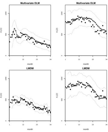
Figure 4: Plots of the one-step forecasts (joined dots) and ±1.96 forecast standard devi-ation error bars (dotted lines) for Xt(1) andXt(2) calculated using the LMDM, together
with the data (filled dots).
Figure 4 shows plots of the time series forXt(1) andXt(2), together with the (marginal)
one-step forecasts and±1.96 (marginal) forecast standard deviation error bars calculated using both the MV DLM and the LMDM. From these plots, it can be seen that the LMDM is performing better than the MV DLM. This is also clearly reflected in the MSE/MAD values for the one-step ahead forecasts for the two models, shown in Table 1. Also shown in Table 1 are the MSE/MAD values for the two- and three-step ahead forecasts using
both models. Clearly, the LMDM is also performing better with respect to these k-step ahead forecasts.
MSE MAD
MV DLM LMDM MV DLM LMDM
One-step forecasts Xt(1) 3541.72 1601.39 26.89 23.26
Xt(2) 4622.96 3988.42 49.31 40.77
Two-step forecasts Xt(1) 4579.25 1513.81 27.71 23.56
Xt(2) 5486.01 3998.98 51.96 37.86
Three-step forecasts Xt(1) 3854.69 1509.43 39.54 22.51
Xt(2) 7198.47 4145.12 68.43 39.56
Table 1: MSE and MAD values for the MV DLM and LMDM.
In addition to giving a better forecast performance, the LMDM also has the advantage that intervention can be simpler to implement. For example, suppose that total sales of the brands were expected to increase suddenly. Then to accommodate this information into the model, only intervention for Yt would be required in the LMDM, whereas the
MV DLM would require intervention for both Xt(1) and Xt(2). The LMDM also has
the advantage that only observation variances need to be elicited, whereas the MV DLM has the additional difficult task of eliciting the observation covariance between Xt(1) and
Xt(2) as well.
3
Simple calculation of marginal forecast covariances
From Queen and Smith (1993), the marginal forecast covariance between Yt(i) andYt(r),
i < r,r= 2, . . . , n, can be calculated recursively using,
cov(Yt(i), Yt(r)|Dt−1) = E (Yt(i)·E (Yt(r)|Yt(1), . . . , Yt(r−1), Dt−1)|Dt−1) −E(Yt(i)|Dt−1)E(Yt(r)|Dt−1). (3.1) In this paper we shall use this to derive a simple algebraic form for calculating these forecast covariances. In what follows let at(r) be the prior mean forθt(r).
Theorem 1 In an LMDM, let Yt(j1), . . . , Yt(jmr) be the mr parents of Yt(r). Then for
i < r, the one-step ahead forecast covariance between Yt(i) and Yt(r) can be calculated
using
cov(Yt(i), Yt(r)|Dt−1) =
mr
X
l=1
where at(r)(jl) is the element of at(r) associated with the parent regressor Yt(jl) — ie
at(r)(jl) is the prior mean for the parameter for regressorYt(jl).
Proof. Consider Equation 3.1. From the observation equations for the LMDM, E (Yt(r)|Yt(1), . . . , Yt(r−1), Dt−1) =Ft(r)Tat(r).
Also, using the result that for two random variables X and Y, E(Y) = E(E(Y|X)), E (Yt(r)|Dt−1) = E¡Ft(r)Tat(r)|Dt−1¢= E¡Ft(r)T|Dt−1¢at(r).
So
cov(Yt(i), Yt(r)|Dt−1) = E(Yt(i)·Ft(r)T|Dt−1)at(r)−E(Yt(i)|Dt−1)E(Ft(r)T|Dt−1)at(r)
= cov(Yt(i),Ft(r)T|Dt−1)at(r).
NowYt(r) has themr parents Yt(j1), . . . , Yt(jmr), so
Ft(r)T =¡
Yt(j1) · · · Yt(jmr) xt(r)
T ¢
where xt(r)T is a vector of known variables. Then, cov(Yt(i),xt(r)T|Dt−1) is simply a vector of zeros and so
cov(Yt(i), Yt(r)|Dt−1) =
mr
X
l=1
cov(Yt(i), Yt(jl)|Dt−1)at(r)(jl)
as required.
The marginal forecast covariance betweenYt(i) and Yt(r) is therefore simply the sum
of the covariances betweenYt(i) and each of the parents ofYt(r). Consequently it is simple
to calculate the one-step forecast covariance matrix recursively.
Corollary 1 In an LMDM, let Yt(j1), . . . , Yt(jmr) be the mr parents of Yt(r). Suppose
that the series have been observed up to, and including, time t. Define
at(r, k) =E(θt+k(r)|Dt)
so that
at(r, k) =Gt+k(r)at(r, k−1)
with at(r,0) = mt(r), the posterior mean for θt(r) at time t. Denote the parameter
associated with parent regressor Yt(jl) by θt(r)(jl), and E(θt+k(r)(jl)|Dt)by at(r, k)(jl), the
Then, for i < r and k ≥ 1, the k-step ahead forecast covariance between Yt+k(i) and
Yt+k(r) can be calculating recursively using
cov(Yt+k(i), Yt+k(r)|Dt) = mr
X
l=1
cov(Yt+k(i), Yt+k(jl)|Dt)at(r, k)(jl).
Proof. LetXt+k(r)T =¡ Yt+k(1) . . . Yt+k(r−1) ¢. Using the result thatE(XY) =
E[X·E(Y|X)],
cov (Xt+k(r), Yt+k(r)|Dt) = E(Xt+k(r)·E(Yt+k(r)|Yt+k(1), . . . , Yt+k(r−1), Dt)|Dt) −E(Xt+k(r)|Dt)E(Yt+k(r)|Dt). (3.2) From DLM theory (see, for example, West & Harrison (1997), pp 106–7),
E(Yt+k(r)|Yt+k(1), . . . , Yt+k(r−1), Dt) =Ft+k(r)Tat(r, k) (3.3)
where
at(r, k) =Gt+k(r)at(r, k−1)
with at(r,0) =mt(r), the posterior mean forθt(r) at timet. Also,
E(Yt+k(r)|Dt) = E[E(Yt+k(r)|Yt+k(1), . . . , Yt+k(r−1), Dt)]
= E[Ft+k(r)Tat(r, k)|Dt] by Equation 3.3. Thus Equation 3.2 becomes,
cov(Xt+k(r), Yt+k(r)|Dt) = cov(Xt+k(r),Ft+k(r)T|Dt)at(r, k) and so theith row of this gives us
cov(Yt+k(i), Yt+k(r)|Dt) = mr
X
l=1
cov(Yt+k(i), Yt+k(jl)|Dt)at(r, k)(jl),
as required.
Corollary 2 For two root nodesYt(i) and Yt(r), under the LMDM,
cov(Yt(i), Yt(r)|Dt−1) = 0. Proof. From the proof of Theorem 1,
Since Yt(r) is a root node,Ft(r) only contains known variables so that,
cov(Yt(i),Ft(r)T|Dt−1) = 0.
The result then follows directly.
To illustrate calculating a one-step forecast covariance using Theorem 1 and Corol-lary 2, consider the following example.
Example 1 Consider the DAG in Figure 1. Forr= 2, . . . ,5 andj= 1, . . . ,4, letat(r)(j)
be the prior mean for parent regressor Yt(j) in Yt(r)’s model. The forecast covariance
betweenYt(1) andYt(5), for example, is then calculated as follows.
cov(Yt(1), Yt(5)|Dt−1) = cov(Yt(1), Yt(4)|Dt−1)at(5)(4)+ cov(Yt(1), Yt(3)|Dt−1)at(5)(3)
cov(Yt(1), Yt(4)|Dt−1) = cov(Yt(1), Yt(3)|Dt−1)at(4)(3)
cov(Yt(1), Yt(3)|Dt−1) = cov(Yt(1), Yt(1)|Dt−1)at(3)(1)+ cov(Yt(1), Yt(2)|Dt−1)at(3)(2).
Yt(1) andYt(2) are both root nodes and so their covariance is 0. So,
cov(Yt(1), Yt(5)|Dt−1) = var(Yt(1)|Dt−1)at(3)(1)
³
at(4)(3)at(5)(4)+at(5)(3)
´
.
where var(Yt(1)|Dt−1) is the marginal forecast variance for Yt(1). This is both simple and
fast to calculate. ¥
When a DAG has a logical node, the logical node will be some (logical) function of its parents. If the function is linear, then the covariance betweenYt(i) and a logical node
Yt(r) will simply be a linear function of the covariance between Yt(i) and the parents of
Yt(r). For example, for the DAG in Figure 5, suppose that Yt(4) =Yt(3)−Yt(2). Then
cov(Yt(1), Yt(4)|Dt−1) = cov(Yt(1), Yt(3)|Dt−1)−cov(Yt(1), Yt(2)|Dt−1).
The covariance can then be found simply by applying Theorem 1.
4
Component covariances
Suppose that Yt(r) has the mr parents Yt(r1′), . . . , Yt(rm′ r) for r = 2, . . . , n. Write the
observation equation for each Yt(r) as the sum of regression components as follows.
Yt(r) = mr
X
l=1
Yt(r, r′l) +Yt(r,xt(r)) +vt(r), vt(r)∼N(0, Vt(r)) (4.1)
with
Yt(r, r′l) = Yt(r′l)θt(r)(r
′
l)
Yt(r,xt(r)) = xt(r)Tθt(r)(xt(r))
whereθt(r)(r
′
l) is the parameter associated with the parent regressorY
t(rl′) andθt(r)(xt(r))
is the vector of parameters for known variablesxt(r). It can sometimes be helpful to find the covariance between two components Yt(i, i′) and Yt(r, r′) from the models for Yt(i)
and Yt(r) respectively. Call cov(Yt(i, i′), Yt(r, r′)) the component covariance for Yt(i, i′)
and Yt(r, r′). We shall illustrate why component covariances may be useful by considering
two examples.
Example 2 Component covariances in traffic networks
Queenet al. (2007) consider the problem of forecasting hourly vehicle counts at various points in a traffic network. The possible routes through the network are used to elicit a DAG for use with an LMDM. It may be useful to learn about driver route choice probabilities in such a network — i.e. the probability that a vehicle starting at a certain point A will travel to destination B. Unfortunately, these are not always easy to estimate from vehicle count data. However, component covariances could be useful in this respect, as illustrated by the following hypothetical example.
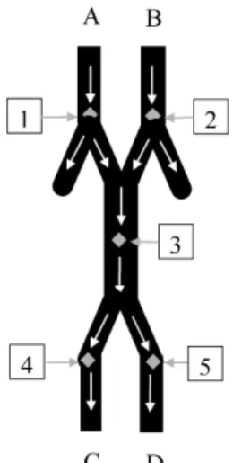
Consider the simple traffic network illustrated in Figure 6. There are five data collec-tion sites, each of which records the hourly count of vehicles passing that site. There are four possible routes through the system: A to C, A to D, B to C and B to D. Because all traffic from A and B to C and D is counted at site 3, it can be difficult to learn about driver route choices using the time series of vehicle counts alone.
Let Yt(r) be the vehicle count for hour t at site r. A suitable DAG representing the
conditional independence relationships between Yt(1), . . . , Yt(5) is given in Figure 7. (For
Figure 6: Hypothetical traffic network for Example 2 with starting points A and B and destinations C and D. The grey diamonds are the data collection sites, each of which is numbered. White arrows indicate the direction of traffic flow.
at site 3 flow to sites 4 or 5 so that conditional on Yt(3) andYt(4), Yt(5) is a logical node
with Yt(5) =Yt(3)−Yt(4).
Figure 7: DAG representing the conditional independence relationships between
Yt(1), . . . , Yt(5) in the traffic network of Figure 6.
From Figure 6, Yt(3) receives all its traffic from sites 1 and 2, while Yt(4) receives all
its traffic from site 3. So possible LMDM observation equations for Yt(3) and Yt(4) are
given by,
Yt(3) = Yt(1)θt(3)(1)+Yt(2)θt(3)(2)+vt(3), vt(3)∼N(0, Vt(3)),
Yt(4) = Yt(3)θt(4)(3)+vt(4), vt(4)∼N(0, Vt(4)).
where 0≤θt(3)(1), θt(3)(2), θt(4)(3)≤1. Then
Yt(1)θt(3)(1) = Yt(3,1) = number of vehicles travelling from site 1 to 3 in hourt,
Yt(3)θt(4)(3) = Yt(4,3) = number of vehicles travelling from site 3 to 4 in hourt.
So cov(Yt(3,1), Yt(4,3)) is informative about the use of route A to C. A high correlation
C and a small correlation indicates a low probability. Of course, the actual driver route choice probabilities still cannot be estimated from these data. However having some idea of the relative magnitude of the choice probabilities can still be very useful. ¥
Example 3 Accommodating changes in the DAG
In many application areas the DAG representing the multivariate time series may change over time — either temporarily or permanently. For example, in a traffic network a temporary diversion may change the DAG temporarily, or a change in the road layout may change the DAG permanently. Because of the structure of the LMDM, much of the posterior information from the original DAG can be used to help form priors in the new DAG (see Queenet al. (2007) for an example illustrating this). In this respect, component covariances may be informative about covariances in the new DAG. We shall illustrate this using a simple example.
Figure 8 shows part of a DAG representing four time seriesYt(1), . . . , Yt(4) (the DAG
continues with children of Yt(3) and Yt(4), but we are only interested inYt(1), . . . , Yt(4)
here). Using an LMDM and Equation 4.1, suppose we have the following observation equations for Yt(3) and Yt(4):
Yt(3) = Yt(3,1) +vt(3), vt(3)∼N(0, Vt(3)), (4.2)
Yt(4) = Yt(4,1) +Yt(4,2) +vt(4), vt(4)∼N(0, Vt(4)). (4.3)
Figure 8: Part of a DAG for Example 3 for four time seriesYt(1), . . . , Yt(4).
Now suppose that the DAG is changed so that a new series,Xt, is introduced which lies
between Yt(1) and Yt(4) in Figure 8. Suppose further thatYt(1) and Yt(4) are no longer
observed. The new DAG is given in Figure 9 (again the DAG continues, this time with children ofYt(3),Xtand Yt(2)). The componentYt(3,1) from Equation 4.2 is informative
about Yt(3) in the new model, and the component Yt(4,1) from Equation 4.3 is
informa-tive about Xt in the new model. Thus the component covariance cov(Yt(3,1), Yt(4,1)) is
Figure 9: New DAG for Example 3 (adapting the DAG in Figure 8) whereXtis introduced
into the DAG and Yt(1) and Yt(4) are no longer observed.
The following theorem presents a simple method for calculating component covariances. Theorem 2 Suppose thatYt(i′) is the parent ofYt(i) andYt(r′) is a parent ofYt(r), with
i < r. Then,
cov(Yt(i, i′), Yt(r, r′)|Dt−1) =cov(Yt(i′), Yt(r′)|Dt−1)at(i)(i
′)
at(r)(r
′)
where at(i)(i
′)
and at(r)(r
′)
are, respectively, the prior means for the regressor Yt(i′) in
Yt(i)’s model and the regressor Yt(r′) in Yt(r)’s model.
Proof. For eachr, let Z(r)
t T
=¡
Yt(r, r1′) Yt(r, r2′) . . . Yt(r, rm′ r) Yt(r,xt(r)) vt(r)
¢
and
Zt(r)T =³ Z(1)
t T
Z(2)
t T
. . . Z(r−1)
t
T ´
.
Using the result that for two random variables X and Y, E(XY) = E(X·E(Y|X)), we have, for a specific r′ ∈ {r′
1, . . . , r′mr},
cov(Zt(r), Yt(r, r′)|Dt−1) = E(Zt(r)·E(Yt(r, r′)|Zt(r), Dt−1)|Dt−1)
−E(Zt(r)|Dt−1)E(Yt(r, r′)|Dt−1). (4.4) Now, from Equation 4.1,
E(Yt(r, r′)|Zt(r), Dt−1) = E(Yt(r, r′)|Yt(1), . . . , Yt(r−1), Dt−1) =Yt(r′)at(r)(r
′)
.
Also,
E(Yt(r, r′)|Dt−1) = E[E(Yt(r, r′)|Zt(r), Dt−1)] = E(Yt(r′)at(r)(r
′)
So, Equation 4.4 becomes,
cov(Zt(r), Yt(r, r′)|Dt−1) = E(Zt(r)Yt(r′)at(r)(r′)|Dt−1)
−E(Zt(r)|Dt−1)E(Yt(r′)at(r)(r′)|Dt−1) = cov(Zt(r), Yt(r′)|Dt−1)at(r)(r′).
The single row from Zt(r) corresponding toYt(i, i′) then gives us,
cov(Yt(i, i′), Yt(r, r′)|Dt−1) = cov(Yt(i, i′), Yt(r′)|Dt−1)at(r)(r
′)
. (4.5)
Let
Xt(r, i)T =¡ Yt(1) Yt(2) . . . Yt(i−1) Yt(i+ 1) . . . Yt(r−1) ¢. Then
cov(Xt(r, i), Yt(i, i′)|Dt−1) = E(Xt(r, i)·E(Yt(i, i′)|Xt(r, i), Dt−1)|Dt−1)
−E(Xt(r, i)|Dt−1)E(Yt(i, i′)|Dt−1). (4.6) Now,
E(Yt(i, i′)|Xt(r, i), Dt−1) =Yt(i′)at(i)(i
′)
,
and Equation 4.6 becomes
cov(Xt(r, i), Yt(i, i′)|Dt−1) = cov(Xt(r, i), Yt(i′)|Dt−1)at(i)(i′). So taking the individual row ofXt(r, i) corresponding toYt(r′) we get,
cov(Yt(r′), Yt(i, i′)|Dt−1) = cov(Yt(r′), Yt(i′)|Dt−1)at(i)(i
′)
.
Substituting this into Equation 4.5 gives us
cov(Yt(i, i′), Yt(r, r′)|Dt−1) = cov(Yt(i′), Yt(r′)|Dt−1)at(i)(i
′)
at(r)(r
′)
as required.
Theorem 2 allows the simple calculation of the component correlations. For example, in Example 2,
cov(Yt(3,1), Yt(4,3)|Dt−1) = cov(Yt(1), Yt(3)|Dt−1)at(3)(1)at(4)(3)
Corollary 3 Suppose thatYt(i′) is the parent ofYt(i)andYt(r′)is a parent of Yt(r), with
i < r. Then, using the notation presented in Corollary 1, for i < r and k≥1, the k-step ahead forecast covariance between components Yt+k(i, i′) and Yt+k(r, r′) can be calculating
recursively using
cov(Yt+k(i, i′), Yt+k(r, r′)|Dt) = mr
X
l=1
cov(Yt+k(i′), Yt+k(r′)|Dt)at(i, k)(i
′)
at(r, k)(r
′)
.
Proof. This is proved using the same argument to that used in the proof of The-orem 2, where t is replaced by t+k and noting the E(θt+k(i)(i
′)
|Dt) = at(i, k)(i
′)
and E(θt+k(r)(r
′)
|Dt) =at(r, k)(r
′)
.
5
Covariance between root nodes
Recall from Corollary 2 that the covariance between two root nodes is zero in the LMDM. However, this is not always appropriate. For example, consider the traffic network in Example 2. Both Yt(1) and Yt(2) are root nodes which may in fact be highly correlated
— they may have similar daily patterns with the same peak times, etc, and they may be affected in a similar way by external events such as weather conditions.
One possible way to introduce non-zero covariances between root nodes is to add an extra node as a parent of all root nodes in the DAG. This extra node represents any variables which may account for the correlation between the root nodes.
Example 4 In the traffic network in Example 2, suppose thatXtis a vector of variables which can account for the correlation betweenYt(1) andYt(2). So, Xt might include such
variables as total traffic volume entering the system, hourly rainfall, temperature, and so on. Then Xt can be introduced into the DAG as a parent of Yt(1) and Yt(2) as in Figure 10.
Figure 10: DAG representing time series of vehicle counts in Example 4, with an extra node Xtto account for any correlation between Yt(1) andYt(2).
applying Theorem 1 we get,
cov(Yt(1), Yt(2)|Dt−1) = var(Xt|Dt−1)at(1)(Xt)at(2)(Xt)
where at(2)(Xt)
and at(2)(Xt)
are the prior mean vectors for regressorsXt inYt(1) and
Yt(2)’s model. ¥
6
Concluding remarks
In this paper we have presented a simple algebraic form for calculating the one step ahead covariance matrix in LMDMs. We have also introduced a simple method for calculating covariances between regression components of different DLMs within the LMDM. Com-ponent covariances may be of interest in their own right, and may also prove to be useful for forming informative priors following any changes in the DAG for the LMDM. Their use in practice now needs to be investigated in further research.
One of the problems with the LMDM is the imposition of zero covariance between root nodes. To allow nonzero covariance between root nodes we have proposed introducingXt into the model as a parent of all the root nodes, where Xt is a set of variables which may help to explain the correlation between parents. Further research is now required to investigate how well this might work in practice.
Acknowledgements
We would like to thank the reviewer for their very useful comments on an earlier version of this paper and also Unilever Research for supplying the data.
References
Cowell, R.G., Dawid, A.P., Lauritzen, S.L. and Spiegelhalter, D.J. (1999) Probabilistic Networks and Expert Systems. Springer Verlag: New York.
Dawid, A.P. (1979) Conditional independence in statistical theory (with discussion). Jour-nal of the Royal Statistical Society,41, 1–31.
Farrow, M. (2003) Practical building of subjective covariance structures for large compli-cated systems. The Statistician,52, No. 4, 553–573.
Farrow, M., Goldstein, M. and Spiropoulos, T. (1997) Developing a Bayes linear decision support system for a brewery. In The Practice of Bayesian Analysis (eds S. French and J. Q. Smith), pp. 71-106. London: Arnold.
Fosen, J., Ferkingstad, E., Borgan, ∅., and AalenFosen, O.O. (2006) Dynamic path
anal-ysisa new approach to analyzing time-dependent covariates. Lifetime Data Analysis, 12 (2), 143–167.
Goldstein, M., Farrow, M. and Spiropoulos, T. (1993) Prediction under the influence: Bayes linear influence diagrams for prediction in a large brewery. The Statistician, 42, No. 4, 445-459.
Queen, C.M. (1994) Using the multiregression dynamic model to forecast brand sales in a competitive product market. The Statistician,43, No. 1, 87–98.
Queen, C. M. (1997) Model elicitation in competitive markets. InThe Practice of Bayesian Analysis (eds S. French and J. Q. Smith), pp. 229-243. London: Arnold.
Queen, C.M., Smith, J.Q. and James, D.M. (1994) Bayesian forecasts in markets with overlapping structures. International Journal of Forecasting,10, 209–233.
Queen, C.M. and Smith, J.Q. (1993) Multiregression dynamic models. Journal of the Royal Statistical Society, Series B,55, 849–870.
Queen, C.M., Wright, B.J. and Albers, C.J. (2007) Eliciting a directed acyclic graph for a multivariate time series of vehicle counts in a traffic network. Australian and New Zealand Journal of Statistics To appear.
Sun, S.L., Zhang, C.S. and Yu, G.Q. (2006) A Bayesian network approach to traffic flows forecasting. IEEE Transactions on Intelligent Transportation Systems,7 (1), 124–132. Tebaldi, C., West, M. and Karr, A.K. (2002) Statistical analyses of freeway traffic flows.
Journal of Forecasting,21, 39-68.
West, M. and Harrison, P.J. (1997) Bayesian Forecasting and Dynamic Models (2nd edi-tion) Springer-Verlag. New York.
Whitlock, M.E. and Queen, C.M. (2000) Modelling a traffic network with missing data.