Brownstein_unc_0153D_14117.pdf

(1)

ANALYSIS OF TIME-TO-EVENT DATA, INTERMEDIATE PHENOTYPES, AND SPARSE FACTORS IN THE OPPERA STUDY

Naomi C. Brownstein

A dissertation submitted to the faculty of the University of North Carolina at Chapel Hill in partial fulfillment of the requirements for the degree of Doctor of Philosophy in

the Department of Biostatistics.

Chapel Hill 2013

Approved by:

Eric Bair

Jianwen Cai

Michael Kosorok

Gary Slade

(2)

c 2013

(3)

ABSTRACT

NAOMI C. BROWNSTEIN: Analysis of Time-to-event Data, Intermediate Phenotypes, and Sparse Factors in the OPPERA Study

(Under the direction of Drs. Eric Bair and Jianwen Cai)

Motivated by the Orofacial Pain: Prospective Evaluation and Risk Assessment

(OPPERA) project, a large study of temporomandibular disorders (TMD), this dissertation

develops statistical methods applicable to three facets of chronic pain.

First, we propose a method for parameter estimation in survival models with missing

censoring indicators. These result because conducting multiple invasive examinations

for incidence on all participants in large prospective studies is infeasible. We estimate

the probability of being an incident case for those lacking a gold standard” examination

using logistic regression. Multiple imputations of case status for each missing examination

are generated using these estimated probabilities. Imputed and observed data are

combined in Cox models to estimate the incidence rate and associations with putative

risk factors. The variance is estimated using multiple imputation. Our method performs

as well as or better than competing methods and highlighted new discoveries for

OPPERA.

Secondly, we propose a general method to analyze secondary phenotypes and apply

it to the OPPERA baseline case-control study. Traditional case-control genetic association

studies examine relationships between case-control status and one or more covariates.

Investigators now commonly study additional phenotypes and their association with

the original covariates as secondary aims. Assessing these associations is statistically

(4)

interest. Standard methods may be biased and lack coverage and power. Utilizing

inverse probability weighting and bootstrapping for standard error estimation, our

method performs as well as competitors when they are applicable and provides promising

results for outcomes to which other methods do not apply.

Third, we propose a method for sparse factor analysis. Psychometric studies frequently

measure numerous variables that may be noisy manifestations of a few underlying

constructs. Aims include identifying these latent variables and their relationship to

the observed variables and reducing the data to a few key variables that explain the

majority of variance. While variable reduction methods exist for principal component

analysis, none have been proposed to date for factor analysis. Our method retains

predictive accuracy for many thresholds in simulations while providing sparse loadings.

(5)

To my little sister, Shira Brownstein, in loving memory. Both her presence and

absence have shaped my progress throughout the program and continue to inspire me

(6)

ACKNOWLEDGMENTS

People commonly say that it takes a village to raise a child. It also takes a villiage to

complete a PhD. There are numerous individuals to whom I owe gratitude in regards to

this endeavor. I apologize in advance to any individuals I have inadvertently omitted.

First and foremost, I am deeply appreciative of my co-advisors, Drs. Eric Bair

and Jianwen Cai. Both have shaped me immeasurably throughout my time at UNC,

providing not only technical insight on the research, but serving as caring mentors and

encouraging me to work hard and develop to my full potential. This dissertation would

not have been completed, especially not in this time frame, without their dedication

and support. Secondly, I am grateful for the committee members, namely Drs. Michael

Kosorok, Gary Slade and Donglin Zeng, for taking the time to meet with me and provide

helpful questions and comments that strengthened the research. I also appreciate the

staff at UNC, such as Melissa Hobgood, Veronica Stallings, Christine Kantner, and

especially Mae Beale and Dean Barbara Rimer, without whom I likely would not have

finished this degree.

Peers have been invaluable, as we’ve navigated through this journey together.

Thank you to Steve Hoberman, Lan Liu, Amy Richardson, Joe Rigdon, and Eugene

Urrutia, among others, for studying together in courses and qualifying exams, creating

a cooperative atmosphere in which to grow as statisticians, and for your friendship.

Thank you to those who came or finished beforehand and offered helpful advice, such

as Eric Daza, Beth Horton, Diana Lam, Che Smith, and Alison Wise, and Drs. John

(7)

Leann Long, and Greg Mayhew.

My graduate study was made financially possible by generous support from the NSF

Graduate Research Fellowship Program grant #0646083 and NIH/NIEHS T32ES007018,

led by Dr. Amy Herring. I would like to acknowledge and thank the principal

investigators of the OPPERA study for providing the data which was analyzed in

this dissertation. Specifically, this includes Drs. William Maixner, Luda Diatchenko,

Bruce Weir, Richard Ohrbach, Roger Fillingim, Joel Greenspan, and Ronald Dubner.

The OPPERA study was supported by NIH/NIDCR grant U01DE017018.

Finally, I am grateful for the vast emotional support of family and friends. Thank

you to my parents, sisters, grandparents, and extended family, for being here for me

throughout the many ups and downs of this time. I especially appreciate the company

of and opportunity to become closer with the Reed family. Thank you to the many

friends who offered advice, comfort and joy when it was most needed including, but not

limited to Jessica Meed and Bronco Suzuki, Charlotte and Michael Hall, Laenja and

Matt Brackett, Elizabeth Clendinning, Paul Baek, Anthony Kuhns, Correai Moore,

Jonathan Rowell, Alyssa Manning, and many others on the UNC Ballroom Dance

Team and in UNC Hillel. Last but not least, thank you to Jesse Haskins for supporting

me, especially around the qualifying exam and during our year of long distance while

I completed the dissertation. I look forward to beginning the next chapter of our lives

(8)

TABLE OF CONTENTS

LIST OF TABLES . . . xi

LIST OF FIGURES . . . xv

1 INTRODUCTION . . . 1

2 LITERATURE REVIEW . . . 4

2.1 Survival Analysis . . . 4

2.1.1 Cox Proportional Hazards Model . . . 5

2.2 Bootstrapping . . . 6

2.2.1 Standard Error and Confidence Intervals . . . 7

2.3 Missing Data: General Theory and Methods . . . 8

2.3.1 The EM Algorithm . . . 10

2.3.2 Multiple Imputation . . . 10

2.3.3 Bootstrapping and Missing Data . . . 11

2.4 Missing Data Methods and Survival Analysis . . . 12

2.4.1 Cox Models with Missing Covariates . . . 13

2.4.2 Cox Models with Missing Censoring Indicators . . . 13

2.5 Genetics and Case-Control Data . . . 17

2.6 Sparse Factor Analysis . . . 19

3 PARAMETER ESTIMATION IN COX PROPORTIONAL HAZARD MODELS WITH MISSING CENSORING INDICATORS . . . 22

3.1 Introduction . . . 22

(9)

3.3 Model . . . 25

3.3.1 Notation and Assumptions . . . 25

3.3.2 Estimating Event Probabilities . . . 27

3.3.3 Multiple Imputation . . . 27

3.3.4 Estimation of Incidence . . . 29

3.4 Simulations . . . 30

3.5 Analysis of the OPPERA Study . . . 34

3.5.1 Hazard Ratios . . . 35

3.5.2 Incidence Rates . . . 37

3.6 Discussion . . . 38

4 MODELING SECONDARY PHENOTYPES CONDITIONAL ON GENOTYPES IN CASE-CONTROL STUDIES . . . 44

4.2 Proposed Method . . . 47

4.3 Simulation Study . . . 49

4.3.1 General Setup . . . 49

4.3.2 Continuous Phenotypes . . . 50

4.3.3 Ordinal Phenotypes . . . 51

4.3.4 Time-to-Event Phenotypes . . . 54

4.4 Data Application . . . 54

5 SPARSE FACTOR ANALYSIS . . . 61

5.2 Proposed Methodology . . . 62

5.2.1 Notation . . . 62

(10)

5.2.3 Our Algorithm . . . 65

5.3 Simulations . . . 66

5.4 Data Application . . . 69

5.4.1 The Baseline Case-Control Study of Chronic TMD . . . 70

5.4.2 Application to the Full OPPERA Cohort . . . 73

6 CONCLUSION . . . 94

APPENDIX 1: SUPPLEMENTARY MATERIAL FOR CHAPTER 3 . . . 96

APPENDIX 2: SUPPLEMENTARY MATERIAL FOR CHAPTER 5 . . . 114

(11)

LIST OF TABLES

3.1 Simulation Results for MAR . . . 41

3.2 Results from the OPPERA Study . . . 42

3.3 Estimated TMD Incidence Rates With and Without

Imputation . . . 43

4.1 Results of Simulations for Intermediate Continuous

Phenotypes . . . 52

4.2 Results of Simulations for Intermediate Ordinal Phenotypes . . . 59

4.3 Results of Simulations for Intermediate

Time-to-Event Phenotypes . . . 60

5.1 Parameters for Different Thresholds and Other Methods . . . 79

5.2 P-Values for Different Thresholds and Other Methods . . . 80

5.3 Number of Variables Retained for Different Thresholds

and Other Methods . . . 81

5.4 PCA/SFA QST Results for Controls, c=0.4 . . . 82

5.5 Autonomic Parameter Estimates and Different

Thresholds, Component 2 . . . 83

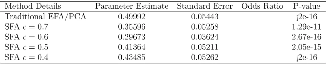
5.8 Autonomic Results for the OPPERA Case Control

Study, c=0.7 . . . 86

5.9 PCA/SFA QST Results for the Entire OPPERA

Cohort, c=0.8 . . . 87

5.10 PCA/SFA Autonomic Results for the OPPERA

(12)

Thresholds for Component 1, First-Onset TMD . . . 89

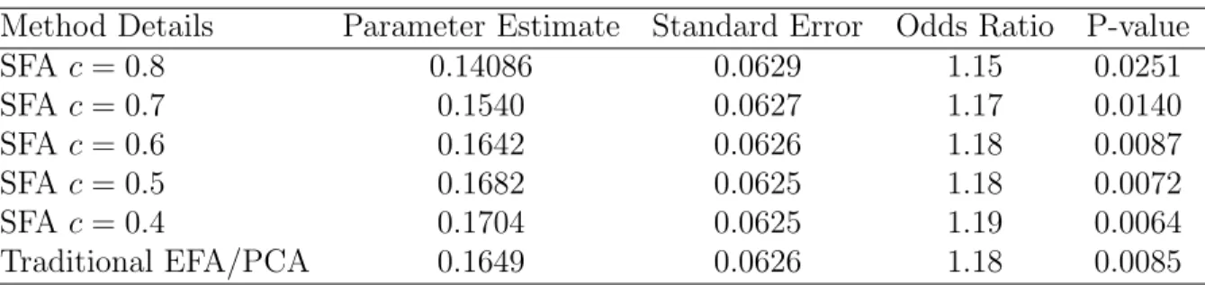
5.12 PCA/SFA Psychosocial Results for the Entire OPPERA Cohort, c=0.6 . . . 90

5.13 Psychosocial Parameter Estimates and Different Thresholds, Component 1 (Chronic) . . . 91

A1.1 Simulation Results for MCAR . . . 103

A1.2 Simulation Results for MCAR . . . 104

A1.3 Results for an Extra Covariate Included in the Logistic Regression Model . . . 105

A1.4 Results when a Relevant Covariate is Omitted frin the Logistic Regression Model . . . 106

A1.5 Results when the Logistic Regression Model is Applied to Observations with Qi = 0 . . . 107

A1.6 Results when an Extra Covariate is Included in the Logistic Regression Model and the Model is Applied to Observations with Qi = 0 . . . 108

A1.7 Results when a Relevant Covariate is not Included in the Logistic Regression Model and the Model is Applied to Observations where Qi = 0 . . . 109

A1.8 Simulation Results for MNAR, scenario A . . . 110

A1.9 Simulation Results for MNAR, scenario B . . . 111

A1.10Simulation Results for Poisson Models, MAR . . . 112

A1.11Simulation Results for Incidence Rates . . . 113

(13)

A2.2 PCA/SFA QST Results for the Entire OPPERA

Cohort, c=0.5 . . . 116

Cohort, c=0.6 . . . 117

Cohort, c=0.7 . . . 118

A2.5 PCA/SFA QST Results for the OPPERA

Follow-up Cohort, c=0.4 . . . 119

A2.10PCA/SFA Autonomic Results for the OPPERA

Followup Cohort, c=0.4 . . . 124

A2.14PCA/SFA QST Results for Cases, c=0.4 . . . 128

A2.15Autonomic Results for the OPPERA Case Control

Study, c=0.4 . . . 129

Study, c=0.5 . . . 130

(14)

Study, c=0.8 . . . 132

A2.19PCA/SFA Psychosocial Results for the Entire

OPPERA Cohort, c=0.4 . . . 133

OPPERA Cohort, c=0.4 to 0.55 . . . 136

OPPERA Cohort, c=0.6 to 0.45 . . . 137

(15)

LIST OF FIGURES

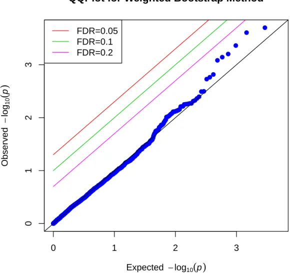
4.1 QQ Plot for the Unweighted Method . . . 57

(16)

CHAPTER 1: INTRODUCTION

Time-to-event analyses are frequently conducted in medicine, actuarial science, and

numerous other fields of applied science. Actuaries study the time until death of

individuals for the purpose of calculating and offering fair life insurance rates. In

clinical trials, researchers note whether and when participants experience the event of

interest and compare the times between the treatment and control groups. Similarly,

in cohort studies, researchers compare survival times and want to know if survival time

is related to a risk factor of interest. Additionally, it may be of interest to study the

hazard of death over time.

There is a well-developed set of standard time-to-event analysis methods implementable

in standard statistical software packages. Logrank tests allow testing of differences of

survival times between a finite number of groups. The survival distribution may be

eassily estimated non-parametrically and plotted using SAS or R. Semi-parametric

methods, such as the Cox proportional hazards model, allow robust estimation of the

hazard function in the presence of covariates. Yet, these methods require knowledge

of both the event time and status for all individuals. The event status may not be

known for all individuals, especially when one is interested in studying death due to a

particular cause.

Additionally, current methods do not work for secondary time-to-event outcomes

in case-control studies, in which study participants are sampled based on the primary

(17)

of interest. In fact, arbitrary analysis of one or more secondary phenotypes is a

non-trivial problem and has spawned a great deal of research in recent years.

Often, the outcome of interest may be difficult to ascertain. For example, an

autopsy by expert medical examiner may be needed to determine if a death was due

to myocardial infarction, a cancer tumor, or other factors. In order to mitigate this

problem, some studies employ delayed event adjudication. That is, possible cases are

identified using simple, but possibly error-prone methods. Then, one or more experts

examines the possible cases using a more accurate, but also more costly and

time-consuming method to determine the true event status. For example, a specialized

dental examination is required for accurately diagnosing temporomandibular disorders

(TMD). It is impractical to subject large number of subjects to such an examination,

especially if they are unlikely to have the condition. Instead, the “gold standard”

examination is performed only on subjects who screen positive on a simpler assessment,

such as a questionnaire designed to measure recent orofacial pain. However, some

subjects do not receive the “gold standard” examination due to inability or unwillingness

to attend research centers. A time-to-event analysis would then have some subjects

with self-reported symptoms but missing censoring indicators. This setting presents

statistical challenges, which require care in order to avoid bias and maintain efficiency.

In other settings, cause of death may be unknown or death certificates may be

missing entirely. This frequently arises when there are multiple failure types. In

oncology studies, for example, researchers may want to differentiate between deaths

due to cancer and deaths due to car accidents or other unrelated causes. For such

studies, a death certificate is insufficient to classify a subject. Moreover, it may be

impossible to determine if a death occurred if a subject dies abroad or national death

registries are incomplete.

(18)

There is a clear need for new methodology to handle this challenging situation. In

the first paper, we propose a method for parameter estimation in the case of missing

censoring indicators. In the second paper, we seek an unbiased and efficient method to

model the relationship between a genotype and a secondary phenotype in case-control

studies. The third paper extends the framework of the first paper to allow for Cox

(19)

CHAPTER 2: LITERATURE REVIEW

Our methods, detailed in chapters 3-5, rely on basic knowledge of survival analysis,

missing data, imputation, bootstrapping, joint-modeling, case-control genetic studies

and factor analysis. This chapter reviews the literature pertaining to these fields.

2.1 Survival Analysis

Actuaries, medical experts, and statisticians alike are frequently confronted with

failure time data. One important quantity of interest is the survival function. The

nonparametric maximum likelihood estimate of the survival distribution is given by

(60). Nonparametric estimation in the accelerated failure time model is discussed in

(72). The shape of the survival function is instructive in studying the progression of

the event of interest over time.

Yet, it is often of interest to model the relationship between the failure times and

a set of covariates. A parametric model with one covariate assuming that the failure

time has an exponential distribution is proposed in (36). Unfortunately, the stringent

distributional assumption and limit of one covariate prevent this method from being

useful in most situations. Instead, the classic semi-parametric model of the hazard

function in the presence of covariates is defined in (10). The field of survival analysis

in the past forty years has been centered around this model. In fact, in prospective

(20)

approximate the incident rate ratio. The pervasiveness of this model is evident in, for

example, (40), a review of developments in survival analysis in clinical trials through

the turn of the century.

2.1.1 Cox Proportional Hazards Model

One of the most popular statistical tools today, the Cox model combines the ability

to handle covariates with the flexibility resulting from leaving the baseline hazard

unspecified. Cox defines a partial likelihood, which allows for maximum likelihood

estimation of the regression parameters, and extends results for bivariate life table

data. Further details on the partial likelihood are provided in (11).

The Fisher information matrix for the regression parameter from the standard

likelihood is calculated in (26) and shown under broad conditions to be asymptotically

equal to the information based on the partial likelihood. Thus, the Cox likelihood is

asymptotically efficient. Efron also estimates the hazard rate and connects it to the

Kaplan-Meier estimate of the survival function. Accelerated failure time model and

inference and parameter estimation in the Cox model is discussed in (59) as well as

extensions to multivariate failure data, time-dependent covariates, and case control

studies. A heuristic method for computing the asymptotic variance of the estimated

survival function is proposed in (68) and used it to construct confidence intervals, which

are shown in simulations to have adequate coverage.

The applicability of Cox models continued to grow. Methodology were generalized

to competing risks and multivariate outcomes. The framework for competing risks is

detailed in (81), (50) and (94).

Another important question is how robust the Cox model is to mis-measured or

missing data and what modifications are appropriate in the presence of such data.

(21)

with missing data are discussed in section 2.4. Specifically, the setting of uncertain

outcomes are discussed in section 2.4.2.

2.2 Bootstrapping

Bootstrapping is an estimation method that may be applied in a wide variety of

situations with or without missing data. The goal is to estimate a statistical quantity

and its variability. Bootstrapping is especially useful for quantities whose standard

error is difficult or impossible to calculate mathematically. Over the past 30 years, the

original method has evolved dramatically, with new methods applicable to frequentist,

Bayesian, parametric, nonparametric, and semiparametric situations alike.

The nonparametric bootstrap was originally proposed in (27) as a modification of

the jackknife. The first step is to find the empirical distribution function of the data.

Next, one creates a large number of boostrap samples by sampling with replacement

from this empirical distribution function. Third, one combines the results from each of

the replications. The estimate of the quantity of interest is the mean of theRestimates

from the replicates and the estimated standard error is the standard deviation of the

estimates from the replicates. Details may be found in (27) and (29).

This simple procedure, available in standard statistical software, originally allowed

estimation of the parameter of interest and of bias, but now also routinely provides

several confidence intervals. Asymptotic properties, including second order accuracy,

are discussed in (111), (5) and (112). Literature on standard errors and confidence

interval estimation is discussed in more detail in section 2.2.1.

In its classical form, bootstrapping is a nonparametric frequentist method, though

it has been adapted to the parametric and Bayesian frameworks as well. One example

(22)

distribution for the unknown sampling distribution, Efron substitutes a normal distribution

with mean and variance equal to the sample mean and sample variance. This procedure

is called the normal smoothed bootstrap. (102) first described the Bayesian bootstrap.

Weighted bootstrapping, which is applicable to hypothesis testing, is discussed in (62).

Bootstrapping has emerged as a useful tool for practitioners and the foundation of

numerous papers on its theoretical properties, scope, and limitations.

In his silver anniversary review paper, (31) stresses that boostrapping is founded

on the “plug-in principle”, which he defines as the act of simply “plugging in” the

empirical distribution function for the unknown distribution function. He notes that

while the literature as of 2003, (19), indicates that this is generally valid to the second

order, there are notable situations where it can be problematic. According to a similar

review paper by (14), it is the simplicity of the bootstrap and its connection with other

methods, such as the jackknife, that make it both widely utilized in applications and

extensively studied from a theoretical standpoint.

2.2.1 Standard Error and Confidence Intervals

One important benefit of bootstrap methods is the ability to calculate standard

errors and confidence intervals. For many estimators of interest in practice, standard

errors are, at best, difficult to calculate, or worse, impossible to evaluate analytically.

Moreover, even when the standard error can be found, standard confidence intervals

based on the central limit theorem may be inadequate for statistics whose distribution

are non-normal. On the other hand, according to (32), the bootstrap can always provide

numerical standard error estimates. A simple example of the bootstrapping in the Cox

proportional hazards model can be found in (32).

(23)

namely percentile, bias corrected and acclerated (BCa), approximate bootstrap confidence

intervals (ABC) and bootstrap ‘t’. The percentile method simply reports the estimated

percentiles of the bootstrap distribution. A quick theoretical justification for percentile

intervals is provided in (28). BCa intervals are motivated by the assumption that a

simple monotone transformation of the parameter of interest is normally distributed

with slight bias with respect to the transformed mean and a variance that may not

be constant for all possible parameter values. The user does not need to specify the

transformation. In order for BCa confidence intervals to be accurate, it is only required

that such a transformation exists. Monte Carlo sampling yields adequate estimates of

the standard error in about 50-200 replications for most statistics and adequate BCa

confidence intervals in about 1000 replications (32, 19). The bootstrap ‘t’ interval is

conceptually simpler than BCa intervals. However, unlike percentile intervals, they are

not transformation invariant and can result in confidence intervals that are much too

wide. ABC intervals do not require Monte Carlo simulations at all, relying instead on

an analytic approximation to the BCa interval.

2.3 Missing Data: General Theory and Methods

The problem of missing data is nearly ubiquitous in practical statistical problems.

Consequently, there is a rich body of research on analysis with missing data, including

methods such as the EM algorithm, single imputation, and multiple imputation. There

are also a wide variety of ad-hoc techniques that may introduce severe bias. This section

summarizes the literature on missing data and proper data analyses.

In the classic paper, (101) defines three missing data mechanisms and ignorability.

Before proceeding, necessary definitions from Rubin’s work are introduced. Additional

(24)

of having missing data. Data are called missing completely at random (MCAR) if

the probability of having a missing value is independent of the data, both observed

and missing. Data are called missing at random (MAR) if the probability of having a

missing value is independent of the missing values, but may depend on the observed

values or on observed covariates. Under MAR or MCAR, the missing data mechanism

is said to be ignorable. If the probability of having a missing value depends on that

unobserved value, then the data is missing not at random (MNAR) and the mechanism

is non-ignorable.

When confronted with missing data, data users face a dilemma. They may know

that, in theory, disregarding observations that are not fully observed is inefficient, at

best. The loss in efficiency increases with the proportion of missing data. It may

bias inference and lead to misleading conclusions. Yet, most software is not equipped

to handle missing observations. Typically, observations with any missing values are

dropped. This can be problematic in studies with a large number of covariates of

interest. Subjects with one or more of the covariates missing would be excluded.

Denoted a “complete-case” analysis, the results may be severely biased when the

missing data mechanism is non-ignorable. Similarly, “available-case” analyses, which

use all cases with observed values for at least one of the variables under consideration,

may be invalid. Mean-imputation, in which missing values are imputed by the mean of

observed values, may also introduce bias, (103). While it may be tempting to use these

or other more convenient approaches, it is usually not appropriate. There is a rich set

of methodology for handling missing data without introducing bias and maintaining as

(25)

2.3.1 The EM Algorithm

One common method for handling missing data is the Expectation-Maximization

(EM) Algorithm. There are three steps: first, finding the expected value of the

full log-likelihood given the observed data and current parameter estimate, second

maximizing the expectation to update the parameter estimates, and third, iterating

until convergence. The method was formally introduced in (16) with details of the

E-step and M-E-step. The authors demonstrate why the EM algorithm works, that is, the

fact that the likelihood always increases with each iteration. They also give examples

and suggest the ability to generalize the EM algorithm in a Bayesian framework.

The EM-algorithm in some form is instrumental in most papers that develop new

methods for analysis of data with missingness. One noteworthy example is in the

context of logistic regression with uncertain outcomes. The EM-algorithm and known

or estimated values of sensitivity and specificity are used in (74) to improve upon

parameter estimates in standard logistic regression. Section 2.4 discusses additional

examples of methods that employ the EM-algorithm for missing data in survival analysis.

2.3.2 Multiple Imputation

Multiple imputation, discussed in section 2.3, is a Bayesian method for analyzing

data with some degree of missingness. It was first presented as a way to handle

non-response in sample surveys. The framework is summarized in (103) as containing

a database constructor often separate from the person who will analyze data. He

states that multiple imputation is a statistically valid method within this framework.

Multiple imputation definitions and equations are reviewed. He defines proper multiple

(26)

Finally, Rubin compares multiple imputation to competing methods, i.e. single imputation,

jackknife, bootstrapping.

Missing data mechanisms are discussed in (155) from frequentist and Bayesian

points of view as well as the consequent challenges under various assumptions and

appropriate missing data analysis methods. Imputation in general is explored in (155),

specifically two multiple imputation methods – propensity score and predictive model

– under monotone missingness, and one method of multiple imputation under

non-monotone missingness utilizing Markov Chain Monte Carlo (MCMC). Readily vailable

multiple imputation software procedures, such as PROC MI and PROC MIANALYZE

in SAS, frequently assume data are MAR.

Often, especially for binary data, values generated with multiple imputation are

rounded. Yet, rounding can cause excessive bias, as shown in (51). One solution is

to keep the raw imputed values, as they introduce less bias than the rounded values.

They urge instead to posit a more appropriate posterior, for example to refer to Rubin’s

detailed instructions for how to impute missing binary data.

2.3.3 Bootstrapping and Missing Data

For missing data problems, (30) provides a comparison of three bootstrapping

methods and multiple imputation. Non-parametric bootstrapping, the simplest form

of bootstrapping, requires no knowledge of the missing data mechanism. It may be

applied to virtually any reasonable estimator. However, nonparametric bootstrapping

may be too slow or infeasible to use in practice due to the comparatively large number

of replications required. This is especially true when BCa confidence intervals are of

utmost interest.

(27)

of the missing data mechanism. Thus, it is most appropriate for non-ignorable missing

data, when this is required anyway. The multiple-imputation bootstrap begins with

the Bayesian bootstrap and calculates confidence intervals via the ABC method. It is

most appropriate for Bayesian settings, because it requires knowledge of the conditional

density of the full data given the observed data. Note that the requirement to know the

conditional density is less stringent than the requirement of full-mechanism bootstrapping

to know the missing data mechanism. For censored surival data, full mechanism and

nonparametric bootstrapping are identical (29, 30).

An important type of partially incomplete data is censored failure-time data. Under

the assumption of random censoring, (29) argues that bootstrapping is valid for survival

data. Similarly, it is straightforward to use bootstrapping to estimate the survival

function and its standard error.

2.4 Missing Data Methods and Survival Analysis

This section discusses specific developments in missing data methods for

time-to-event data. As discussed previously, survival analysis already has incomplete data in

the sense that the failure time is unknown for censored individuals. Most methods

assume that data are censored randomly. In the literature, this is termed as ignorable

censoring. When this assumption is not tenable, censoring is termed non-ignorable and

adjustments must be made.

When modeling time-to-event data with covariates, there are additional types of

missing data that may arise. Most commonly, some subjects may have one or more

unobserved covariates. A less studied situation is when the censoring indicator is

missing for a subset of the observations. While it is possible for a single dataset to

(28)

have been found to date.

The following subsections detail, respectively, the literature for survival analysis

with missing covariates and missing censoring indicator models.

2.4.1 Cox Models with Missing Covariates

There have been numerous papers on modeling proportional hazards with missing

covariates. Estimating equations are propposed in (65) to yield what they call an

“approximate partial likelihood estimator” (APLE), which is consistent and asymptotically

normal under MCAR covariates. The assumption is relaxed to MAR by (89) and

impute the covariates using the conditional expectation based on observed information.

Through simulations, they demonstrate the superiority of their method to that of

Lin and Ying in terms of efficiency under MCAR and consistency under MAR. A

nonparametric model for estimation of relative risk with the missing covariates is given

in (156) based on additional auxiliary covariates. An EM-type algorithm for missing

covariates in Cox models is detailed in (49). Additional papers include the inverse

selection probability weighted estimator of (139), among others.

2.4.2 Cox Models with Missing Censoring Indicators

Missing censoring indicators frequently arise when there are multiple failure types.

Investigators may easily record the mortality of all subjects, but it may be extremely

difficult or costly to find out exactly why each subject died. Consequently, there has

been much more work done on missing censoring indicators in the context of competing

risks than when there is only one type of failure. Over the past three decades, authors

(29)

for the missing censoring indicator model. The logrank test has been generalized for

missing censoring indicators. Yet, there have been fewer papers on the more difficult

problem of Cox regression.

First, (20) uses the EM algorithm to estimate the survival function under various

types of partially observed competing risk data. Observations may be either fully

observed, censored, or observed failures with unobserved causes. He estimates the

information matrix and provide clear examples of the method applied in practice. The

survival function is estimated non-parametrically in (96) when death status is known

but its cause is uncertain for some subjects, while the Kaplan-Meier estimate may be

biased for such data. Causes of failure are said to be masked when it is unknown but

at least one type of cause may be eliminated from consideration. For competing risks

data with masked causes of failure, (39) estimate the survival function.

A modified logrank test for competing risk data for which cause of failure is unknown

and missing at random, (44). A slight modification to their partial likelihood is

proposed in (17) to increase the information and improve the test. Multiple imputation

of the cause of failure and a corresponding asymptotically valid modified log-rank test

is detailed in (133).

For standard survival data, there have been a number of methods proposed for

estimating the survival function under the missing censoring indicator model. An

asymptotically efficient estimator of the survival function under missing at random,

or more generally, “coarsening at random” censoring indicators, is proposed by (136).

Namely, they use the nonparametric MLE of the survival function based on reduced

data produced by a discretization of the failure time. A comparable alternative is

proposed by (123) that requires less computational resources and time. Kernel estimation

is employed in (124) to provide a weakly convergent estimator of the survival function.

(30)

the choice of bandwidth sequence. It follows that clever estimation of the bandwidth

would improve the kernel estimation performance. Three methods of bootstrapping the

bandwidth are compared to each other and to existing methods, (129). Semiparametric

random censorship models for hazard function estimatiors, both nonparametric and

semiparametric, are given in (128). In addition, they compute and minimize the

asymptotic mean squared error to find the optimal bandwidth. An augmented inverse

probability weighted estimator of the survival function under MAR is proposed in

(127) and shown that it is robust even under partial model misspecification. Improving

the survival function estimate in the missing censoring indicator model via multiple

imputation is discussed in (125) and (126).

An important research question is how Cox models are affected when case status

is uncertain. Competing risks proportional hazards regression models are proposed

in (45) using estimating equations assuming that observations are known either to be

censored or to have failed by some cause. They assume proportional hazards for each

failure type and between the two failure types. For the linear transformation model,

An augmented inverse probability weighted estimator and algorithm are proposed in

(41) along with asymptotic and double robustness properties.

Time-to-event data which may not be classified and confirmed is modeled in (8)

by weighting each subject by their estimated probability of being a true case. Their

methods include estimation of the survival function, Cox models, and a logrank test.

They propose an asymptotic variance expression which may be used as an approximation

for finite samples. Alternatively, they suggest estimating the variance by bootstrapping.

Empirical processes are employed to prove consistency and weak convergence of the

estimators to Gaussian processes.

For the usual survival setting with only one cause of failure, (43) estimate the

(31)

estimation in the Cox model and prove consistency and asymptotic normality of the

estimators. The survival function is also estimated without covariates and Cox proportional

hazards models are proposed in (78) by modifying the Nelson-Aelen estimator and

taking the product-integral. The advantage of their method is that it does not require

discretization of the failure times or estimation of the unconditional probability of

having an observed censoring indicator. Simulations demonstrate that the (78) is

superior to previous estimators, such as the earlier version of (43). Yet, the methods

of (78) and (43) both depend on the MCAR assumption, which they state that it is

non-trivial to relax. Parameter estimation in the Cox model under the assumptions of

proportional censorship and MCAR censoring indicators is conducted in (122).

Weights are recommended for each potential event, of which individuals may have

more than one, along with a weighted partial likelihood, (116). That is, he suggests

screening out observations that are unlikely to be true events, and weighting each

observation by the probability that the subject had first failed at the observed time. The

weights may be known or estimated using auxiliary covariates. Taking this uncertainty

into account reduces bias and increases power. However, estimating the weights depends

upon the presence of a normally distributed diagnostic variable and either knowing or

having experts guess the relative frequency of true endpoints to false endpoints. In

addition, the variance of the method is mentioned but not described in detail.

Adjusting a proportional hazards model based on discrete survival times and measurement

error of case status is discussed in (79). They show that mis-measured outcomes can

bias the usual proportional hazards model parameter estimates toward the null and poor

coverage probability for confidence intervals, but this can be mitigated by incorporating

information about sensitivity and specificity.

Estimators for the regression parameters in the Cox proportional hazards model

(32)

their consistency is established under basic regularity conditions. The authors then

estimate the non-missing rate of censoring indicators with the kernel estimator and use

it to estimate the information matrix. Their approach depends on the assumption of

piecewise constant hazard functions and proportional hazards for not only the event

time, but also for the censoring time.

Multiple imputation is also discussed for repeated failure times where the event is

known to have occurred at a certain time but the event type is missing (107). The

method is compared to multiple imputation under the Cox proportional hazards model

without repeated events.

2.5 Genetics and Case-Control Data

Investigators are frequently interested in reusing case-control data to evaluate associations

between measured risk factors and outcomes other than the outcome to define case

status. These other outcomes are often referred to as secondary phenotypes, which may

be associated with the primary disease used to define case status. Utilizing one study

to investigate more than one outcome is important for financial reasons, as the process

of attaining genetic information and other putative risk factors for all participants is

time-consuming and expensive. While logistic regression is known to be invariant to

the sampling method for primary analyses, this does not hold for secondary phenotype

analyses. Simple logistic and linear regression may be severely biased. Restricting

analyses to cases only or controls only results in decreased efficiency. These methods

are considered “naive” methods. There has been a great deal of recent interest in

developing unbiased and efficient methodology for analyzing secondary phenotypes in

case-control studies.

(33)

standard logistic regression model with a covariate adjusting for original case status.

The second is to use stratum-weighted logistic regression, i.e. logistic regression in

which cases and controls are weighted by the reciprocal of their sampling fractions.

For population studies, it is often easier to estimate the ratio of the sampling fractions

than to estimate the sampling fractions for cases and controls separately. Hence, (97)

proposes using a unit weight for the cases and the ratio of the sampling fractions for

controls. In a nested case-control study, the ratio is the number of cases in the whole

study divided by number of controls.

Simulations are conducted in (82) to estimate size and power for the naive methods

and the inverse probability weighting (IPW) method and dummy variable adjustment

method in (97). They conclude that IPW has adequate type I error but has increased

variance and sometimes decreased power compared to the naive approaches. Note,

however, that the simple unweighted analysis and the analyses that adjust for case

status with a binary variable or restrict to either cases or controls have slightly inflated

type I error when the primary disease is not rare and both the genetic profile and

secondary phenotype are related to the primary disease. There are also situations in

which the IPW method is more efficient than the method that adjusts for case-control

status with an indicator variable for case status.

A rigorous likelihood based approach is derived in (66). However, (63) points out

that (66) assumes no interaction between the covariate information (genotypes) and the

secondary phenotype and that in the case of interaction in modeling the probability

of having the primary disease, the results may be biased. They propose an adaptive

weighting parameter estimate motivated by a Bayesian shrinkage estimator for

gene-environment interaction when the disease is rare.

The bias may be corrected by solving iterated non-linear equations relating regression

(34)

and using bootstrapping to calculate confidence intervals via the percentile method,

(140). Their method assumes that the secondary phenotype may be modeled by logistic

regression given a set of binary covariates and the primary disease may be model by

logistic regression given the covariates and the secondary phenotype but no interaction.

They describe the IPW method in (97) and extend it to retrospective case-control

studies using an estimate of disease prevalence. They also adapt their bias correction

method to the frequency-matched case-control study design. Their method produced

narrower confidence intervals than the IPW method.

In their second paper, (141) conduct simulations, which show that the method

in (140) has adequate size and is more powerful than the naive logistic regression

approaches. A joint model based on a Gaussian copula is proposed by (47) for one

or more secondary phenotypes in the exponential family and the disease of interest

given the covariate, i.e. genotype. Their simulations confirm that their method is more

powerful than the IPW method. Unlike other methods, this one allows joint modeling of

multiple secondary phenotypes that is more powerful than multiple univariate analyses.

2.6 Sparse Factor Analysis

Latent variable models are frequently used in statistics. In certain situations, it

is reasonable to assume that observed variables are random variations of one or more

unobserved random variables. Within the field of psychometrics, studies often consist

of a large number of correlated measured variables, which may be manifestations

of a smaller number of underlying constructs. Factor analysis is commonly used

for this purpose. In factor analysis models, the observed data is assumed to be

a linear combination of the unobserved factors, plus random error. See (9) for an

(35)

theoretical description of the problem of factor analysis is provided in (3) along with a

demonstration that it may fall into the Bayesian framework.

Factor analysis may be either exploratory or confirmatory in nature. Exploratory

factor analysis (EFA) aims to discover underlying relationships between the observed

variables and is more commonly used (91). Confirmatory factor analysis (CFA) begins

with an a priori structure and tests hypotheses about those structures using the factor

analysis setting. Researchers such as (137, 55) have debated quite heatedly about when

each type of factor analysis is appropriate.

Principal component analysis (PCA) is more frequently used in statistics than

is factor analysis. In principal component analysis, instead of assuming that there

are unobserved variables driving the observed data, it is desired to extract linear

combinations of the observed variables. The first linear combination, or component,

explains the largest amount of variability in the data. The second component explains

the next largest amount of variance, and so on. Traditionally, principal component

analysis extracts the same number of components as there are observed variables.

However, since data reduction is commonly a goal of PCA, usually the analyst selects

a smaller number of components that explains a sufficient amount of variance.

It is desired to have sparse loadings, meaning that many of the loadings are equal to

zero. Unfortunately, neither principal component analysis nor factor analysis produce

sparse loadings. This can be problematic, especially in genetic settings, where the

number of variables present in the study can be very large. Two methods (157,

147) have recently been proposed for sparse principal component analysis. (147)

uses a penalized matrix decomposition to produce more sparse results than traditional

principal component analysis.

The aforementioned sparse principal component analysis methods do not immediately

(36)

(37)

CHAPTER 3: PARAMETER ESTIMATION IN COX PROPORTIONAL

HAZARD MODELS WITH MISSING CENSORING INDICATORS

3.1 Introduction

Time-to-event analyses are frequently conducted in medicine, actuarial science, and

numerous other fields of applied science. There is a well-developed set of survival

analysis methods implemented in standard software. Semi-parametric methods, such as

the Cox proportional hazards model, allow robust estimation of the effects of covariates

on the hazard function. However, these methods require the analyst to know the

censoring status of each participant, which may not always be available.

In some cases the outcome of interest may be difficult to ascertain. For example, in

oncology studies, researchers may want to differentiate between deaths due to cancer

and deaths due to car accidents or other unrelated causes. Investigators may easily

record the mortality of all subjects, but it may be extremely difficult or costly to find

out exactly why each subject died. One possible solution to this problem is delayed

event adjudication (8). This means that possible cases are not identified immediately

but screened using simple methods that may have poor sensitivity or specificity. Later,

the screened candidate cases are re-examined using a more precise, but also more costly

and time-consuming, method to determine the true event status.

The study that motivates our work is Orofacial Pain: Prospective Evaluation and

Risk Assessment (OPPERA), a prospective cohort study to identify risk factors for the

(38)

study participant was followed for a median of 2.8 years to identify cases of

first-onset TMD. However, it was impractical to perform a physical examination on every

participant. It would also have been inefficient given that most study participants did

not develop the condition. Instead, this “gold standard” examination was performed

only on participants who screened positively on a quarterly screening questionnaire

that was designed to assess recent orofacial pain (1). However, some participants

who screened positively were lost to follow-up before receiving the “gold standard”

examination. Thus a time-to-event analysis would have some participants with missing

censoring indicators.

Cook and Kosorok (8) estimate parameters in Cox proportional hazard models with

missing censoring indicators by weighting observations according to their probability

of being a true case. They show that the estimators are consistent and asymptotically

normally distributed. However, the standard error of their proposed estimate cannot

be easily obtained using existing software without bootstrapping. For the OPPERA

data, a separate Cox model was calculated for each putative risk factor of interest,

including approximately three thousand genetic markers. Consequently, applying this

method to the OPPERA genetic data would be computationally intractable.

In the OPPERA study, the likelihood that a participant who screened positively

was examined was associated with demographic variables such as gender, race, or

socioeconomic status (1). This indicated that the censoring indicators in the OPPERA

study were not missing completely at random (MCAR). Application of models that

assume MCAR censoring indicators may result in biased estimates of hazard ratios for

covariates of interest. More importantly, a participant’s responses to their screening

questions are predictive of whether or not they are an incident case of TMD. This

setting presents statistical challenges, which require care in order to avoid bias and

(39)

methods currently available allow for estimation of the incidence rate. There is a clear

need for new methodology to effectively answer the research questions of the OPPERA

study.

In this paper, we propose a method for parameter and variance estimation in

Cox regression models with missing censoring indicators. The motivating data set

is introduced in section 3.2. We describe our method in section 3.3. In section 3.4, we

report the results of simulations. Finally, in section 3.5 we apply our method to the

OPPERA study. We conclude with a discussion in section 3.6.

3.2 Motivating Data Set: The OPPERA Study

OPPERA is a prospective cohort study designed to identify risk factors for

first-onset TMD. A total of 3,263 initially TMD-free subjects were recruited at four study

sites between 2006 and 2008. TMD status was confirmed by physical examination of

the jaw joints and muscles using the Research Diagnostic Criteria for TMD (25), which

is the gold standard for diagnosing TMD.

Upon enrollment in the study, each OPPERA participant was evaluated for a wide

variety of possible risk factors for TMD, including psychological distress, previous

history of painful conditions, and sensitivity to experimental pain. For a brief overview

of the risk factors of interest in the OPPERA study, see Section 6 in the Web Appendix.

See Ohrbach et al. (86), Fillingim et al. (37), Greenspan et al. (46), and Maixner et al.

(76) for a complete description of the baseline measures that were collected in OPPERA.

After enrollment, each participant was asked to complete questionnaires to evaluate

recent orofacial pain once every three months. These questionnaires (hereafter referred

to as “screeners”) evaluated the frequency and severity of pain in the orofacial region

during the previous three months. The purpose of the screener was to identify participants

(40)

screener, see Slade et al. (114). Participants who screened positively were asked to

undergo a follow-up physical examination by a clinical expert to diagnose presence or

absence of TMD.

Of the 3,263 subjects, 2,737 filled out at least 1 screener, and the remaining 521 did

not fill out any screeners. The total number of screeners was 26,666. There were 717

positive screeners, 486 (about 68%) of which were followed by a clinical examination.

As reported in Bair et al. (1), case classifications made by one examiner (hereafter,

“Examiner #4”) were deemed unreliable because the examiner diagnosed a much higher

percentage of individuals with TMD compared to other examiners. We therefore set

all of Examiner #4’s physical examination findings to be missing and imputed them

using the methods in this paper. This left 404 positive screeners (56%) resulting in

valid clinical exams. On the individual level, after setting the exams from Examiner

#4 to missing, there were 404 people who had one positive screener, and 114 people

who had two or more positive quarterly screening questionnaires.

3.3 Model

3.3.1 Notation and Assumptions

Assume there aren independent participants. For each participanti (i= 1, . . . , n),

let Ci and Ti denote the potential times until censoring and failure, respectively, let

Vi = min(Ti, Ci), ∆i =I(Ti ≤Ci),Ni(t) =I(Ti < t). LetZi ap×1 vector of covariates

measured at baseline and letXi be aq×1 vector of covariates measured at the time of

the putative event. We assume the hazard for participant ifollows a Cox proportional

hazards model

(41)

whereλ0(t) is an unspecified baseline hazard function. Let ξi denote the indicator that

∆i is observed and σi =ξi∆i. We observe (Vi, ξi, σi) fori= 1, . . . , n.

In the OPPERA study,Vi is the length of time for participantibetween enrollment

in the study and either of two events

(a) a screener which resulted in a diagnosis of incident TMD

(b) the last-completed screener before loss-to-follow-up.

If participant i either screened positively and subsequently was diagnosed with TMD,

then ∆i = 1. If participant i either screened negatively on the last quarterly screener

before loss-to-follow up or screened positively and was diagnosed to be free of TMD,

then ∆i = 0. If participant i screened positively on the last screener but was not

examined, then ∆i is missing and ξi = 0. The putative risk factors for TMD that were

assessed at enrollment are denoted by the vector Zi. Responses to the screener for

participant i at time Vi are denoted by the vector Xi. For OPPERA, we also define

Qi = 1 if participant i screens positively on the last screener before either a positive

diagnosis of TMD or loss to follow-up and Qi = 0 otherwise.

We assume the censoring indicators are missing at random (MAR) as follows:

P(ξi = 0|Xi, Vi,∆i, Qi = 1) =P(ξi = 0|Xi, Vi, Qi = 1) (3.2)

In other words, the probability of having a missing censoring indicator may depend on

measured factors, but it does not depend on whether or not an event occurred. We will

(42)

3.3.2 Estimating Event Probabilities

We model the probability that participant iwith a missing censoring indicator is a

case by a logistic regression model based onXi and Vi:

P(∆i = 1|Xi, Vi, Zi, ξi = 0, Qi = 1)

= P(∆i = 1|Xi, Vi, Qi = 1)

= exp(α

0_X

i+γVi)

1 + exp(α0_X

i+γVi)

I(Qi = 1) (3.3)

That is, we estimate the probability of examiner-diagnosed TMD in a participant

who was not examined as intended. (Here I(x) denotes an indicator function.) The

probability was estimated using the time between enrollment and their last positive

screener as well as their answers on that screener. Then, for those individuals who

screened positively on the last screener (i.e. those withQi = 1) and were not examined,

the estimated probability of being a case is estimated by (3.3) with the parameters

replaced by their respective estimates based on individuals who were examined.

Note that if there are repeated measures, we may use a generalized linear mixed

effects logistic regression model rather than a standard univariate logistic regression

model. For example, if some participants screen positively on more than one screener

and are examined at least once, then we have multiple observations per participant.

In that case, fitting a generalized linear mixed effects logistic regression model rather

than a standard logistic regression model would account for correlations between the

responses of the same participant.

3.3.3 Multiple Imputation

One popular method for handling missing data is multiple imputation. For a

(43)

is as follows:

(i) Estimate predicted probabilities as described in the previous section for observations

with missing censoring indicators. These are the individuals who screen positively

but are not examined by a clinician.

(ii) For each observation with a missing censoring indicator, generate a Bernoulli

random variable with success probability equal to the predicted probability found

in step (i).

(iii) Combine the raw data and imputed data from step (ii) to form a completed data

set.

(iv) Fit the Cox proportional hazards model to the completed data set.

(v) Record each parameter estimate ˆβj and covariance matrix ˆUj.

(vi) Repeat steps (ii)-(v) for a total of m times, where m is the desired number of

imputations.

Next, we combine all of the estimates. The average parameter estimate is

¯

β = 1

m m

X

j=1

ˆ

βj, (3.4)

the within-imputation variance estimate is

¯

U = 1

m m

X

j=1

ˆ

Uj, (3.5)

and the between-imputation variance

ˆ

B = 1

m−1

m

X

j=1

(44)

Finally, the estimated covariance matrix is

ˆ

V ar( ¯β) = ¯U+ (1 + 1

m) ˆB. (3.7)

3.3.4 Estimation of Incidence

Previous sections of this paper described how to estimate hazard ratios in the

presence of missing censoring indicators. It may also be of interest to estimate incidence

rates for the same event using Poisson regression instead of Cox regression. For example,

one of the aims of the OPPERA study is to estimate the incidence rate of first-onset

TMD.

In order to estimate incidence rates, we estimate the case probabilities as described

previously based on participants who screened positively and were examined. Then we

impute case status as described in section 3.3.3 for those who screened positively but

were not examined. However, in this case we fit Poisson regression models, rather than

Cox models, to the completed data sets. Finally, we calculate the incidence rate based

on the estimates of the regression coefficients in the Poisson model. Specifically, we use

the data from imputationj to fit the model

log(E(∆ij|Zi, Vi)) = α+β0Zi+ log(Vi) (3.8)

where ∆ij denotes the jth imputation for observation i, j = 1, . . . , m. We combine the

m imputations using equation (3.4) and

¯

α = 1

m m

X

j=1

ˆ

αj. (3.9)

The estimated incidence rate for an individual with covariate Z∗ is given by exp( ¯α+

¯

(45)

3.4 Simulations

Data with missing censoring indicators were simulated, and several possible methods

were compared with respect to bias, coverage, and confidence interval width. Survival

times for 1,000 individuals were generated with exponentially distributed failure times

under a proportional hazards model with covariates as proposed by Bender et al. (4).

That is, the survival time for each individual was distributed according to (3.1) where

λ0(t) = 1 is the baseline hazard. For our simulations, Zi = Xi1 was a single baseline

covariate following a normal distribution with mean 2 and unit variance. In other words,

the failure timesTi followed an exponential distribution with hazard exp(β0Xi1) where

β ∈ {−0.5,−1.5,−3}. The censoring times Ci followed an exponential distribution

with mean 5. This yielded about 35%, 75% and 90% censoring forβ=−0.5,β =−1.5, and β =−3, respectively.

Covariates are represented by Xi1, a risk factor for TMD measured at enrollment,

andXi2, a measurement collected on the last screener. For each observation, a normally

distributed covariate Xi2 was generated with mean ∆i and standard deviation 0.3,

representing a continuous measure of the likelihood of being identified as an incident

case of TMD. This was used to generate Qi = I(Xi2 > 0.5), an indicator of whether

participant i screened positive on their last screener. Also, ξi = I(∆i is observed)

corresponds to the indicator of whether participanti came in for their clinical exam if

Qi = 1. In all simulations, we set ∆i = 0 if Qi = 0 (i.e. the participant’s final screener

was negative). This decision was made to reflect the fact that OPPERA participants

who screened negatively were not examined.

We created missing censoring indicators under the following classical missing data

mechanisms of Rubin (101):

(46)

data. This is known as missing completely at random (MCAR).

(II) The probability of having a missing censoring indicator depends on an observed

covariate. This is known as missing at random (MAR).

(III) The probability of having a missing censoring indicator depends on the (potentially

unobserved) censoring indicator. This is known as missing not at random (MNAR).

Our method assumes that the data are MAR, which includes MCAR as a special

case. Our simulations under MAR and MNAR parallel the study protocol in that

censoring indicators can only be missing for those with positive screeners. In other

words, observations were potentially missing if and only if Qi = 1. (Individuals with

negative screeners have Qi = 0 and are assumed to be censored. Those with positive

screeners haveQi = 1 and may have missing clinical examinations.) Details and results

for MCAR and MNAR data are shown in Sections 6 and 6 in the Web Appendix.

We also considered several simulation scenarios where the logistic regression model for

predicting the censoring indicator was misspecified; see Section 6 in the Web Appendix.

For MAR data, we set censoring indicators to be missing with probability

ρi(Xi, Vi) = P(ξi = 0|Xi, Vi, Qi = 1) (3.10)

= exp(−0.2−0.3Xi1+ 0.1Vi) 1 + exp(−0.2−0.3Xi1+ 0.1Vi)

. (3.11)

In each simulated data set, all observations with observed censoring indicators who

had screened positively were used to fit a logistic regression model for case status with

covariates Xi1, Xi2 and Vi. That is, using the complete data (i.e. observations with

Qi = 1 and ξi = 1), we fit the logistic regression model for the event probability

conditional on X_i0 = (1, Xi1, Xi2) and Vi, namely

(47)

The estimated probabilities ˆpi =

exp( ˆα0_X i+ˆγVi)

1+exp( ˆα0_X

i+ˆγVi) were calculated for individuals with Qi = 1.

To evaluate the performance of our method, multiple imputation was employed

to calculate 100 imputed estimates of β for each simulation as described in Section

3.3.3. For each observation i with Qi = 1 and ξi = 0, we estimated failure indicators

ˆ

∆ij ∼Bernoulli(ˆpi) independently for each imputationj.

A Cox proportional hazards model was fit for each imputed data set, and the

imputed estimates of the regression coefficient and their variances were recorded. These

were aggregated using equations (3.4) and (3.7) to create confidence intervals for the

multiple imputation estimates.

The performance of our method was compared with that of the method of Cook and

Kosorok (8). To obtain the estimates of (8), for each simulated data set, we estimated

the probabilities ˆpi that the (potentially unobserved) event for participant i is a true

event, as described previously. We then fit a weighted Cox proportional hazards model

to the data set. Two new observations were generated for observations with missing

censoring indicators. Each such pair of observations had the same failure time and

covariates, but different failure indicators and weights. The first observation had weight

ˆ

pi and ˆ∆i = 1, and the second observation had weight 1−pˆi and ˆ∆i = 0. Participants

with fully observed data had unit weight. The estimated regression coefficient, ˆβ was

recorded. The variance of this estimate was estimated by generating 1000 bootstrap

replicates of each simulated data set and refitting the model for each bootstrap replicate.

The average parameter estimate, β¯ˆ and percentile confidence intervals (β0.025, β0.975)

were all recorded, whereβα is the αth quantile among the 1000 bootstrap replicates.

We also compared our method to the ideal situation in which all data were observed,

complete case analysis (meaning that we exclude from the data set all observations with

(48)

indicators either all as censored or all as failures. Results under the assumption of MAR

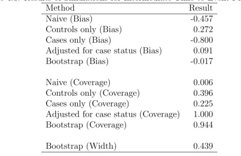
are shown in Table 3.1. We estimated the bias of each method by calculating the mean

difference between the estimated Cox regression coefficient and the true coefficient over

the 1000 simulations. We also calculated the mean width of the confidence intervals

produced by each method over the 1000 simulations. Similarly, we calculated the

empirical coverage probability for the confidence intervals produced by each method by

dividing the number of times that the confidence intervals contained the true value of

the parameter by 1000. Finally, we report the Monte Carlo error for the coverage rate,

which is the error in the empirical coverage probability due to conducting only a finite

number of simulations (which would bepα(1−α)/n for n simulations).

The empirical coverage probability of the imputed confidence intervals is close to

the nominal level (0.95) in all simulations. Our multiple imputation method and the

method of Cook and Kosorok (8) produced approximately unbiased estimates and valid

confidence intervals in all the scenarios we considered. The estimates produced by the

other methods showed a larger amount of bias and did not always achieve the desired

coverage level. Our multiple imputation method also yielded the narrowest confidence

intervals in each scenario, although the method of Cook and Kosorok (8) produced

confidence intervals that were only slightly wider. Moreover, for most parameter values,

the coverage probabilities for the complete case and ad hoc methods were significantly

different (p <0.01) from the nominal rate.

In addition, we examined the performance of our proposed methods when we

changed the logistic regression model for ∆i. We investigate two additional types

of models: one in which the model contained a variable unrelated to case status

and another in which the model does not include one variable related to case status.

As in the previous simulations, the failure times were generated by (3.1), censoring