arXiv:1510.02976v1 [cond-mat.quant-gas] 10 Oct 2015
Hard-Wall and Non-Uniform Lattice Monte Carlo Approaches to
One-Dimensional Fermi Gases in a Harmonic Trap
Casey E. Berger,1,∗ Joaqu´ın E. Drut,1,† and William J. Porter1,‡
1Department of Physics and Astronomy,
University of North Carolina, Chapel Hill, NC, 27599, USA
(Dated: May 16, 2018)
Abstract
We present in detail two variants of the lattice Monte Carlo method aimed at tackling systems in external trapping potentials: a uniform-lattice approach with hard-wall boundary conditions, and a non-uniform Gauss-Hermite lattice approach. Using those two methods, we compute the ground-state energy and spatial density profile for systems ofN = 4−8 harmonically trapped fermions in one dimension. From the favorable comparison of both energies and density profiles (particularly in regions of low density), we conclude that the trapping potential is properly resolved by the hard-wall basis. Our work paves the way to higher dimensions and finite temperature analyses, as calculations with the hard-wall basis can be accelerated via fast Fourier transforms; the cost of unaccelerated methods is otherwise prohibitive due to the unfavorable scaling with system size.
PACS numbers: 03.75.Fk, 67.85.Lm, 74.20.Fg
I. INTRODUCTION
The quantum Monte Carlo method has been around for nearly as long as modern
com-puters (see e.g. Ref. [1–3] for reviews). By far, most calculations that use that method, from
condensed-matter and ultracold-atom systems to quantum chromodynamics, are performed
in uniform lattices with periodic boundary conditions. This approach makes sense in most
of those cases, as the aim is to describe nearly uniform systems, which are such that periodic
boundary conditions minimize finite-size effects. However, this is not always a good
approx-imation in the case of ultracold atoms, where the optical trapping potential plays a central
role in experiments and dictates the many-body properties of the system [4–6]. It is therefore
essential to include a harmonic trap in realistic calculations. As a result of this inclusion,
translation invariance is broken and plane waves on a uniform periodic lattice are no longer
the natural basis of the system. Indeed, in the presence of a trap, momentum ceases to be a
good quantum number. Moreover, the boundary conditions of the true harmonic oscillator
are not at all periodic; in fact, implementing periodicity would result in undesirable copies
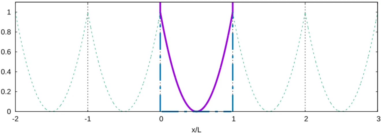
of the harmonic potential across the boundaries (see Figure 1).
0 0.2 0.4 0.6 0.8 1
-2 -1 0 1 2 3
x/L
FIG. 1. Schematic view of a harmonic potential in a one-dimensional box with periodic boundary conditions (dashed lines) as contrasted with the same potential but with hard-wall boundaries (region 0< x/L <1; solid line). The hard-wall potential itself is shown with dashed-dotted lines.
To resolve the above issues, we attempted in Ref. [7] to use the natural coordinate-space
lattice of the harmonic oscillator, namely the Gauss-Hermite points and weights of gaussian
wavefunctions. Although such a non-uniform lattice is physically and mathematically
at-tractive, it is not efficient from the computational standpoint: the scaling with the system
size is prohibitive in more than a single spatial dimension, and there appears to be no simple
way to accelerate those calculations as Fourier transforms do for uniform lattices (there are,
however, possible routes via non-uniform fast Fourier transforms [8]).
In this work, we carry out a test of a methodological compromise between the choices
mentioned above: we return to the uniform-lattice basis, but implement it with hard-wall
boundary conditions (i.e. an infinite square-well potential). The latter prevent the
ap-pearance of spurious copies of the harmonic potential across the boundary, while at the
same time allow for Fourier acceleration (with a small, sub-leading cost of linearly
com-bining the results of Fourier transforms). As a proof of principle, we compute properties
of trapped 1D fermions, namely the ground-state energy and density profiles, and compare
with calculations in the non-uniform basis. Although much is known about fermions in 1D
in uniform space [9], most previous works have combined the classic Bethe-ansatz solution
with the local-density approximation in order to treat trapped systems [10–16]. (See
how-ever Refs. [17–19] for exact-diagonalization approaches.) Our goal here, in contrast, is to
design a more general Monte Carlo method to account for the trapping potential in an ab
initio fashion, which we could apply in higher dimensions.
II. GENERAL OVERVIEW OF THE METHODS
Our calculations explore the properties of a system ofN nonrelativistic, equal-mass, SU(2)
fermions in one spatial dimension under the influence of an external harmonic potential
V0(x) = (1/2)mω2x2 with mass m and trap frequency ω. We take the particles to have
dispersionε(p) =p2/(2m) and to interact via an attractive, pair-wise, short-range potential.
Specifically, we study the Hamiltonian ˆH written
ˆ
H = ˆT + ˆV0+ ˆV (1)
where ˆT is a one-body kinetic energy operator, ˆV0 is coupling to our static background, and ˆ
V is the interparticle potential. Throughout, we work in units where kB =~=m = 1.
In both approaches, we place our system on a discrete spacetime of dimensionless size
well-defined physical volume, and as a result, the length and momentum scales are set by
the frequency ω. Further, for these calculations we choose a nonuniform lattice spacing to
be described in detail below. By contrast, studies performed in the square-well basis are
endowed with a natural volume, and in this instance, we work with a uniform spatial lattice
of size L =Nxℓ, taking ℓ= 1 throughout to fix the relevant scales. Although the details of
the spatial discretization differ between the two approaches, the temporal lattice is uniform
and of dimensionful extent β =Nττ.
We begin, in each method, with a trial state|Ωiand obtain the many-body, ground-state
expectation value of an operator ˆO via large-imaginary-time projection. Specifically, for
eigenfunctions|Eniof ˆH and assuminghE0|Ωiis nonvanishing, it follows from completeness
that
Oβ ≡ h
Ω(β/2)|Oˆ|Ω(β/2)i
hΩ(β/2)|Ω(β/2)i
β→∞
−−−→ hE0|Oˆ|E0i, (2)
where
|Ω(τ)i= ˆU(τ,0)|Ωi, (3)
and where we have defined the imaginary-time evolution operator
ˆ
U(τb, τa) =e
−(τb−τa) ˆH
. (4)
Our representation of each operator comprising ˆH given in Equation (1) is
method-specific, and the details of the lattice Monte Carlo (MC) technique are in each case intuitively
tied to our choice of basis. In both of the methods discussed below, we partition the
Hamiltonian into two noncommuting operators ˆH = ˆH0 + ∆ ˆH, approximating the typical
MC projectors via a symmetric Suzuki-Trotter (ST) decomposition in order to isolate a
single-particle piece ˆH0 whose exponential we can explicitly diagonalize. In the non-uniform
basis method, ˆH0 = ˆT + ˆV0 (diagonal in harmonic-oscillator space), whereas in the uniform
hard-wall basis we take ˆH0 = ˆT (diagonal in momentum space). Generically, we approximate
each factor comprising the evolution operator as
exphτHˆ0+ ∆ ˆH
i
= exp−τ 2Hˆ0
exp−τ∆ ˆHexp−τ 2Hˆ0
+O(τ3) (5)
for small τ.
In both cases, the factors involving ˆH0 are implemented in diagonal form, but in order to
to decouple the central two-body observable. Schematically, we write
exp−τ∆ ˆH=
Z
Dσ(x, τi) exp−∆ ˆHσ(i)
(6)
for each point on the imaginary-time lattice where we have introduced a spatially fluctuating
HS auxiliary fieldσ(x, τi) and a collection of one-body operators ∆ ˆHσ(i). Gathering the path
integrals, we may write the composite evolution operator as an integral over a (now
space-time varying) field as
ˆ
U(β,0) =
Z
Dσ(x, τ) ˆMσ+O(τ2) (7)
where
ˆ Mσ =
1
Y
i=Nτ
exp−τ 2Hˆ0
exp−∆ ˆHσ(i)
exp−τ 2Hˆ0
. (8)
Application of the matrices ˆMσ for a each configuration of the HS field constitutes a sizable
component of the calculation, and by repeatedly switching between two separate bases, the
action of each factor is computed using its diagonal representation. The above sequence of
transformations (Trotter-Suzuki, Hubbard-Stratonovich) leads to the path-integral
represen-tation of Oβ, which we evaluate using Metropolis-based Monte Carlo methods, in particular
hybrid Monte Carlo [22, 23]. Further details are presented below, and for a more complete
discussion see Refs. [1–3].
III. TECHNICAL ASPECTS OF THE METHODS
A. Non-uniform lattice method
Through its connection to gaussian quadrature methods [24, 25], this partition of the
Hamiltonian, or equivalently the choice of which basis functions to use in the
above-mentioned diagonization, provides a natural lattice geometry. Specifically, the need to
resolve the chosen basis states, as well as projections onto them, with high precision
moti-vates a prudent choice of not only the orbitals themselves but also of the integration method.
Expanding a generic trial state demonstrates immediately that in order to guarantee faithful
resolution of this state in terms of single-particle orbitals, it is sufficient to ensure that the
orthonormality of the basis is preserved. We perform our calculations in each case on the
maintain exactly the orthonormality of the single-particle wavefunctions and the fidelity of
our computations expressed thereby.
Written entirely in position space, we have the kinetic energy operator
ˆ
T = X
s=↑,↓
Z
dx ψˆ†
s(x)ε
1 i ∂ ∂x ˆ
ψs(x) (9)
expressed via field operators ˆψs(x) and ˆψ†
s(x) for a state specified by position and spin
quantum numbers (x, s), as well as the two-body contact interaction
ˆ V =−g
Z
dxnˆ↑(x)ˆn↓(x) (10)
given in terms of the density operators ˆns = ˆψs†ψˆs with nonnegative bare coupling g and the
static background potential
ˆ V0 =
X
s=↑,↓
Z
dx V0(x) ˆns(x). (11)
As described in Ref. [7], a convenient basis is the set of single particle orbitals αk(x)
satisfying
− ∂ 2
∂ξ2 +ξ 2
αk= (2k+ 1)αk (12)
for dimensionless variable ξ = √ωx and nonnegative integer k, corresponding to the
har-monic oscillator (HO). Expanding the field operators in terms of creation and annihilation
operators b†k,s and bk,s corresponding to HO quantum numbers (k, s) as
ˆ ψ(†)
s (x) =
∞
X
k=0
αk(x)ˆb(k,s†), (13)
we diagonalize the first two summands comprising ˆH as
ˆ
T + ˆV0 =
X
s=↑,↓
∞
X
k=0
ω
k+ 1 2
ˆb†
k,sˆbk,s. (14)
Using this diagonal form, we perform the calculations using the nonlinear lattice (described
below) by implementing the operator given in Equation (14), in HO space, the remaining
contact interaction ˆV in position space, and switching between throughout the application
of Equations (7),(8). In order to efficiently represent the HO single-particle orbitals αk(x)
in coordinate space, we place the system on a lattice corresponding to Nx Gauss-Hermite
uniform discretization associated with calculations performed using a basis of momentum
eigenstates.
Indeed, a real-valued function f(x) sampled on an n-site GH lattice may be numerically
integrated (see Refs. [24,25]), often to exceptional accuracy, via
Z ∞
−∞
dx f(x)e−x2
= n
X
i=1
wif(xi) +
n!√π 2n(2n)!f
(2n)(ζ) (15)
with weights
wi =
2n−1n!√π
n2 [H
n−1(xi)]2
, (16)
for real ζ, and where the values xi are determined by the roots of the n-th order Hermite
polynomial Hn(x). These conditions are derived by requiring the sum in Equation (15) to
exactly reproduce the desired integral when the function f is taken to be a polynomial of
degree degf < 2n. By choosing to represent our system in coordinate space on a Nx-site
spatial lattice, we maintain exactly that the first Nx HO orbitals form an orthonormal set.
B. Uniform lattice with hard-wall boundary method
Although the previous approach is attractive in its elegant preservation of system’s
un-derlying structure even after discretization, its scaling, particularly in comparison to
conven-tional Fourier-accelerated MC approaches (see Ref. [26, 27]), places discouraging limits on
this method’s applicability vis-`a-vis higher dimensional systems. In any dimension, the
scal-ing is determined by the computational cost of matrix-vector operations, which naively scales
quadratically in the lattice volume, that is O(V2) forV =Nd
x. Accelerated calculations
us-ing a uniform lattice, however, achieve scalus-ing as benign asO(V lnV) [7]. Additionally, the
Fourier-transform basis is naturally orthonormal on a uniform lattice making it all the more
appealing.
Computational cleverness and simplicity aside, the basis functions associated with
conven-tional uniform-lattice techniques exhibit boundary conditions that differ dramatically from
those characterizing eigenstates of the system at hand. For any finite system size,
decom-position in periodic functions fails to capture the required asymptotic behavior, specifically
that the density must be localized in space and must eventually vanish monotonically as
the distance from the trap’s center grows. Although they do not exhibit the same type of
square well (SW), that is a system confined by a hard-wall (HW) trapping potential, do
vanish at the system’s boundaries. Further, even though the GH lattice is defined to
repre-sent functions defined on the entire real line, for any finite lattice size, it inevitably fails to
capture effects coming from the long-distance tails where the discrete representation of the
function is no longer supported. Judicious use of this technique circumvents the problem
almost entirely, as these omissions are minimal when the function of interest is localized
near the origin.
In light of the above, we propose studying a harmonically trapped gas using a large
uniform lattice, in the sense that L√ω ≫1, but rather than making use of the conventional
plane-wave decomposition, we work in a basis of SW wave functions φn(x) for positive
integers n, supported for 0< x < L, and defined by
φn(x) =
r
2 Lsin
nπx
L
. (17)
Expanding the field operators in terms of Fock-space operators which destroy (respectively,
create) a SW state with quantum numbers (n, s), denoted a(n,s, as†)
ˆ ψ(†)
s (x) =
∞
X
n=1
φn(x)ˆa(†)
n,s, (18)
we may diagonalize the kinetic energy operator alone to find
ˆ
T = X
s=↑,↓
∞
X
n=1
p2
n 2m ˆa
†
n,sˆan,s (19)
where we have written the SW momenta as pn = πn/L. As is conventionally done, we
apply the remaining operators, those derived from the interparticle interaction and from the
presence of the background potential, in position space where they are diagonal after the HS
transformation. Since φn(x) is a linear combination of (conventional, complex-exponential)
plane waves, it is straightforward to take advantage of fast Fourier transform algorithms to
accelerate these HW calculations. Indeed, that linear combination relating φn to complex
exponentials involves only 2d terms, i.e. it is a sparse operation whose scaling is only linear
with the lattice volume V = Nd
x. In particular, it scales more favorably than a general
-4 -3 -2 -1 0 1 2 3
0 1 2 3 4 5 6
E/(N
ω
)
2aHO/a0 -7
-6 -5 -4 -3 -2 -1 0 1 2
0 1 2 3 4 5
E/E
FG,HO
2aHO/a0 SHO N = 2
HW N = 2 SHO N = 4 HW N = 4 SHO N = 6 HW N = 6 SHO N = 8 HW N = 8
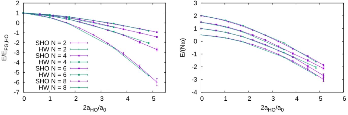
FIG. 2. Energy per particle in units of the energy of the non-interacting case (left panel) and in units of the harmonic-oscillator energy ~ω (right panel), for N = 2,4,6,8 particles (bottom to
top), as obtained with the harmonic-oscillator basis (SHO) and uniform hard-wall basis (HW).
IV. RESULTS AND DISCUSSION
To tune the bare coupling in our lattice calculations, we first computed the ground-state
energy of the two-body problem. Doing so allowed us to read off the value of the continuum
physical coupling (as given by the inverse scattering length 1/a0), as the exact solution of the
two-body system in a harmonic trap can be obtained exactly and is well-known [28]. Having
fixed the target physics in that fashion, for both methods, we were able to meaningfully
compare the results obtained with each of them for higher particle number. In Figure2, for
instance, we show our results for the coupling tuning procedure (N = 2), which are exact
by definition, along with results obtained for higher particle numbers (N = 4,6,8) for those
couplings.
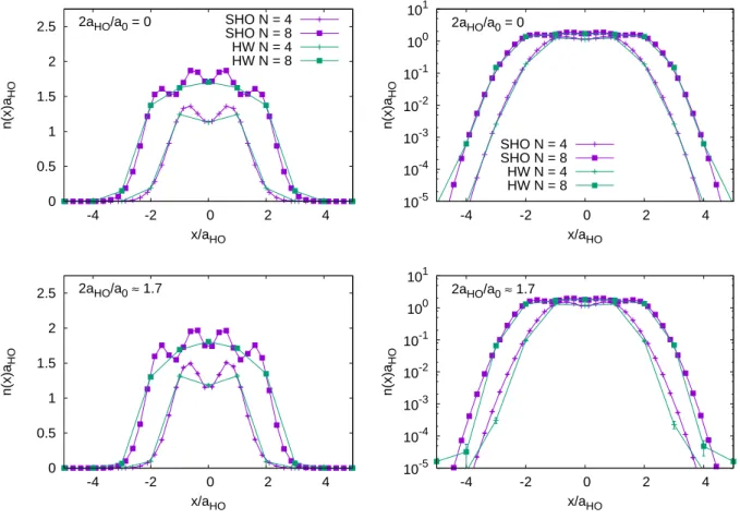
Figure3shows density profiles for noninteracting systems ofN = 4 and 8 particles, along
with their counterparts for an interacting case at 2aHO/a0 ≃ 1.7. The left panels in that
figure show the profiles in a linear scale, whereas the right panels show them in a y-log
scale. In all cases we see that, whenever thex axis values coincide (or do so approximately)
the results for density have the expected values, i.e. the two approaches agree
quantita-tively. The logarithmic plots also show excellent agreement; more precisely, we see that the
long-distance tails (in each direction) decay in a parabolic form, which indicates that the
distances that parabolic form is lost for the hard-wall data, which is not surprising given
the presence of the walls.
0 0.5 1 1.5 2 2.5
-4 -2 0 2 4
2aHO/a0 = 0
n(x)a
HO
x/aHO
SHO N = 4 SHO N = 8 HW N = 4 HW N = 8
0 0.5 1 1.5 2 2.5
-4 -2 0 2 4
2aHO/a0≈ 1.7
n(x)a HO x/aHO 10-5 10-4 10-3 10-2 10-1 100 101
-4 -2 0 2 4
2aHO/a0 = 0
n(x)a
HO
x/aHO SHO N = 4 SHO N = 8 HW N = 4 HW N = 8
10-5 10-4 10-3 10-2 10-1 100 101
-4 -2 0 2 4
2aHO/a0≈ 1.7
n(x)a
HO
x/aHO
FIG. 3. Density profiles for noninteracting systems (top) and interacting (bottom). The left panels display the data in lineary scale, while the right panels show ay-log scale. In all cases we show results for N = 4 and 8 particles, and for the harmonic-oscillator basis (SHO) and uniform hard-wall basis (HW).
V. SUMMARY AND CONCLUSIONS
In this paper, we have presented two methods to address the problem of interacting
fermions in harmonic traps: a uniform-lattice method with hard-wall boundary conditions,
and a non-uniform Gauss-Hermite lattice method (which we had used in previous work).
While the latter has many attractive features (it diagonalizes the noninteracting Hamiltonian
exactly), it is not amenable to Fourier acceleration (or at least not easily), which makes it
hard-wall method, on the other hand, shares some of the positive features and can be Fourier
accelerated, as we explained above.
To test the methods against each other, we compared here calculations for 1D attractively
interacting fermions in a harmonic trap. Specifically, we computed the ground-state energy
and density profiles of unpolarized systems of N = 4 and 8 particles. Our results show that
for both the ground-state energy and the density profiles, the methods agree satisfactorily.
For the density profiles, in particular, we note that the expected gaussian decay is reproduced
with the hard-wall basis over multiple orders of magnitude before breaking down at large
distances due to the presence of the wall. From our calculations we conclude that it is
possible to obtain high-quality results using uniform bases with hard-wall boundaries.
Besides the above benefits, the hard-wall method has the advantage that it does not
depend on the precise form of the external potential. Indeed, it is easy to imagine that it
would be a useful method for other trapping potentials that are unbounded at infinity (e.g.
linear or other). Moreover, the hard-wall potential is interesting per se, as experiments with
ultracold atoms can now mimic that kind of configuration as well (albeit with somewhat
rounded corners at the bottom of the trap, which could be introduced quite easily in our
framework).
ACKNOWLEDGMENTS
We acknowledge discussions with E. R. Anderson and with L. Rammelm¨uller. This
material is based upon work supported by the National Science Foundation under Grants
No. PHY1306520 (Nuclear Theory program) and No. PHY1452635 (Computational Physics
program).
[1] F. F. Assaad and H. G. Evertz, Worldline and Determinantal Quantum Monte Carlo Methods for Spins, Phonons and Electrons, in Computational Many-Particle Physics, H. Fehske, R. Shnieider, and A. Weise Eds., Springer, Berlin (2008);
[4] Ultracold Fermi Gases, Proceedings of the International School of Physics “Enrico Fermi”, Course CLXIV, Varenna, June 20 – 30, 2006, M. Inguscio, W. Ketterle, C. Salomon (Eds.) (IOS Press, Amsterdam, 2008).
[5] I. Bloch, J. Dalibard, W. Zwerger, Rev. Mod. Phys.80, 885 (2008).
[6] S. Giorgini, L. P. Pitaevskii, S. Stringari, Rev. Mod. Phys. 801215 (2008). [7] C. E. Berger, E. R. Anderson, J. E. Drut, Phys. Rev. A 91, 053618 (2015). [8] www.nfft.org
[9] X-W. Guan, M. T. Batchelor, C. Lee, Rev. Mod. Phys. 85, 1633 (2013). [10] I. V. Tokatly, Phys. Rev. Lett.91, 090405 (2004).
[11] G. E. Astrakharchik, D. Blume, S. Giorgini, L. P. Pitaevskii, Phys. Rev. Lett. 93, 050402 (2004).
[12] H. Hu, X.-J. Liu, P. D. Drummond, Phys. Rev. Lett. 98, 070403 (2007). [13] G. Orso, Phys. Rev. Lett. 98, 070402 (2007).
[14] P. Kakashvili, C. J. Bolech, Phys. Rev. A 79, 041603(R) (2009).
[15] J.-H. Hu, J.-J. Wang, G. Xianlong, M. Okumura, R. Igarashi, S. Yamada, M. Machida, Phys Rev. B82, 014202 (2010).
[16] S. Schenk, M. Dzierzawa, P. Schwab, U. Eckern, Phys. Rev. B78, 165102 (2008). [17] P. D’Amico, M. Rontani, Phys. Rev. A 91, 043610 (2015).
[18] T. Sowi´nski, M. Gajda, K. Rz¸a˙zewski, EPL 109, 26005 (2015).
[19] E. J. Lindgren, J. Rotureau, C. Forss´en, A. G. Volosniev, N. T. Zinner, New J. Phys. 16, 063003 (2014).
[20] R. L. Stratonovich, Sov. Phys. Dokl.2, 416 (1958). [21] J. Hubbard, Phys. Rev. Lett. 3, 77 (1959).
[22] S. Duane, A. D. Kennedy, B. J. Pendleton, D. Roweth, Phys. Lett. B195, 216 (1987). [23] S. A. Gottlieb, W. Liu, D. Toussaint, R. L. Renken, Phys. Rev. D35, 2531 (1987).
[24] Press, W. H. ,et al.,Numerical Recipes in FORTRAN, (2nd Ed., Cambridge University Press,
Cambridge, England, 1992).
[25] Stoer, J.; Bulirsch, R. Introduction to Numerical Analysis. Springer-Verlag: New York, USA, 2002; pp. 171-180.
[27] C. Davies, G. Batrouni, G. Katz, A. Kronfeld, P. Lepage, P. Rossi, B. Svetitsky, K. Wilson, J. Stat. Phys. 43, 1073 (1986).