BAYESIAN VIRAL SUBSTITUTION ANALYSIS AND COVARIANCE ESTIMATION VIA GENERALIZED FIDUCIAL INFERENCE
Wen Jenny Shi
A dissertation submitted to the faculty of the University of North Carolina at Chapel Hill in partial fulfillment of the requirements for the degree of Doctor of Philosophy in the
Department of Statistics and Operations Research.
Chapel Hill 2015
Approved by: Jan Hannig Corbin Jones Shankar Bhamidi Lu Shu
ABSTRACT
Wen Jenny Shi: Bayesian Viral Substitution Analysis and Covariance Estimation via Generalized Fiducial Inference
(Under the direction of Jan Hannig and Corbin Jones)
With the advances in biology and computing technologies, there have been increasing amount of big bio data awaiting to be analyzed. Aiming to develop statistical tools for omics data, we focus on the problem of viral sequencing data modeling as well a fundamental statistics question with applications in both biology and many other fields. This dissertation is comprised of three major parts.
Motivated by a multi-time sampled, case-control influenza viral population study, in the first part we model the sequencing data of a viral population under a Bayesian Dirichlet mixture distribution. We have developed an efficient clustering scheme that enables us to distinguish treatment causal changes from variation within viral populations. As a proof of concept, we applied our method to a well-studied HIV dataset, and successfully identified known drug resistant regions and additional potential sites. For the influenza data, our algorithm revealed two genome sites with strong evidence of treatment effect.
distribution, which enables us to define a meaningful confidence region for the covariance matrix.
TABLE OF CONTENTS
LIST OF TABLES . . . viii
LIST OF FIGURES . . . ix
1 Introduction . . . 1
2 Viral substitution analysis . . . 3
2.1
Introduction
. . . 32.2 Parametric Bayesian Mixture Framework . . . 6
2.2.1 Sequencing Data . . . 6
2.2.2 Dirichlet Mixture Model . . . 7
2.2.3 Hellinger Distance . . . 9
2.3 Methodology . . . 10
2.3.1 Preprocess . . . 12
2.3.2 Processing . . . 13
2.3.3 Postprocess . . . 16
2.4 Simulation Study . . . 19
2.5 Real Data Analysis . . . 23
2.5.1 Human immunodeficiency virus 1 (HIV-1) . . . 24
2.5.2 H1N1 Influenza A (IVA) . . . 27
2.6 Discussion . . . 38
2.7 Appendix . . . 39
2.7.1 Proof of Theorem 2.1 . . . 39
2.7.2 Additional IVA Ht plots . . . 42
3 Covariance estimation via fiducial inference . . . 58
3.1 Introduction . . . 58
3.2 Generalized fiducial inference . . . 60
3.2.1 Brief background . . . 60
3.2.2 Generalized fiducial distribution . . . 61
3.3 A fiducial approach to covariance estimation . . . 63
3.3.1 Data generating equation . . . 63
3.3.2 Jacobian . . . 64
3.4 Theoretic results . . . 68
3.5 Reversible jump Markov chain Monte Carlo . . . 70
3.5.1 Algorithm flow . . . 71
3.5.2 Jump map . . . 72
3.5.3 Zeroth-order method . . . 73
3.6 Implementation . . . 74
3.6.1 Special Case I: No fixed zero entries inA . . . 74
3.6.2 Special Case II: Clique model . . . 74
3.6.3 General case with sparsity known . . . 76
3.6.4 General case with sparse locations unknown . . . 78
3.7 Discussion . . . 79
3.8 Proofs . . . 80
3.8.1 Proof of Proposition 3.1 . . . 80
3.8.2 Proof of Proposition 3.2 . . . 81
3.8.3 Proof of Proposition 3.3 . . . 82
3.8.4 Proof of Theorem 3.1 . . . 85
3.9 Appendix . . . 89
3.9.1 F¨orstner-Moonen distance (FM-distance) . . . 89
4.1 Introduction . . . 97
4.2 Stochastic models for phylogenetically dependent gene expressions . . . 98
4.2.1 Brownian motion (BM) . . . 99
4.2.2 Ornstein-Uhlenbeck (OU) . . . 100
4.2.3 L´evy processes . . . 102
4.2.4 Parametric bootstrap . . . 103
4.3 Implementation . . . 103
4.3.1 Multi-species multi-tissues Mammalian data . . . 105
4.3.2 BM vs OU . . . 107
4.3.3 Mean shift test . . . 110
4.4 Discussion . . . 110
LIST OF TABLES
2.1 High through-put sequencing count data . . . 6
2.2 Data preprocessing . . . 12
2.3 Simulation result summary . . . 23
2.4 Simulation efficiency summary . . . 24
2.5 H1N1 result using Passages 1, 3, 9, 12, and the end time point data . . . 34
2.6 H1N1 result with Passages 1, 3, 9, and 12 . . . 36
3.1 Jump map (part1) . . . 73
LIST OF FIGURES
2.1 H1N1 experiment setup . . . 5
2.2 Comparing distributions with Hellinger distance . . . 11
2.3 Three steps clustering procedure . . . 14
2.4 Experiment setup for the toy example and HIV-1 dataset . . . 18
2.5 Simulation experimental design . . . 20
2.6 Test 1 Ht plot . . . 22
2.7 HIV-1 Ht plot . . . 26
2.8 H1N1 Seg6E1 Ht plot . . . 28
2.9 H1N1 Seg6E2 Ht plot . . . 29
2.10 S6-822 raw read . . . 30
2.11 H1N1 Seg7E1 Ht plot . . . 31
2.12 H1N1 Seg7E2 Ht plot . . . 32
2.13 S7-91 raw read . . . 33
2.14 H1N1 experiment setup with 12 passages per line . . . 37
2.15 Seg4E1 Ht plot . . . 43
2.16 Seg4E2 Ht plot . . . 44
2.17 Seg5E1 Ht plot . . . 45
2.18 Seg5E2 Ht plot . . . 46
2.19 Seg8E1 Ht plot . . . 47
2.20 Seg8E2 Ht plot . . . 48
2.21 S8-80 raw read . . . 49
2.22 S1-2299 raw read . . . 50
2.23 S1-2303 raw read . . . 51
2.24 S3-2193 raw read . . . 52
2.25 S4-1210 raw read . . . 53
2.26 S5-24 raw read . . . 54
2.28 S5-1103 raw read . . . 56
2.29 S8-819 raw read . . . 57
3.1 Clique example 1 . . . 91
3.2 Clique example 2 . . . 92
3.3 Clique example 3 . . . 93
3.4 General case with sparsity known example 1 . . . 94
3.5 General case with sparsity known example 2 . . . 94
3.6 General case with sparsity known example 3 . . . 95
3.7 General case with sparsity unknown example 1 . . . 95
3.8 General case with sparsity unknown example 2 . . . 96
3.9 General case with sparsity unknown example 3 . . . 96
4.1 Simple phylogeny . . . 98
4.2 BM trace plot . . . 99
4.3 OU trace plot . . . 101
4.4 Mammalian phylogeny . . . 104
4.5 Heat map of mammalian gene expression data . . . 106
4.6 Heat map of gene expression in mammalian brain tissue . . . 107
4.7 Multiple dimensional scaling plot . . . 108
4.8 BM vs OU test . . . 109
CHAPTER 1 Introduction
In recent years, with the advances in data collection technologies and computing, large amounts of data have been and are continuously harvested. There is a critical need for developing powerful analytical tools and extracting the important information embedded. In this dissertation we present several statistical methods developed for analyzing omics data in the field of biology, which may be extended to other fields as well.
In Chapter 2, we focus on modeling the RNA sequencing (RNA-seq) data and detecting drug resistant regions on the genome for viral populations. To describe the RNA-seq read count distributions, we suggest a Bayesian Dirichlet mixture framework. We develop an efficient three-step clustering procedure to generate the mixture clusters without requiring to specify the number of mixture componentsa priori. Our method analyzes data collected from multiple time points and/or under control and treatment environment simultaneously, and compares posterior distributions for the same genomic location across time and treat-ment environtreat-ments. Through simulations we showed that our clustering algorithm is much more efficient comparing to direct Gibbs sampler. We further applied our method to a well-studied HIV-1 dataset and an H1N1 data with two biological duplicates. Our method revealed the most common known drug resistant sites along with a few other interesting genomic locations.
and Hannig, 2012). To sample from the fiducial distribution, we suggest to use Markov chain Monte Carlo (MCMC) methods. In the general case where the sparse structure of the covariate is unknown, we propose an adaptive Reversible Jump MCMC (RJMCMC) that incorporates the zeroth-order method to improve efficiency.
CHAPTER 2
Viral substitution analysis
2.1
Introduction
RNA viruses and retroviruses, such as SARS, influenza, hepatitis C, polio, and HIV, use RNA as their genetic material. The RNA polymerases of these viruses lack the proof-reading ability of DNA polymerases, which results in a high mutation rate in these RNA genomes and a high rate of genome evolution. This rapid rate of evolution can be advantageous for the virus as it can confound the immune system and lead to the emergence of resistance to antiviral drugs (Boutwell et al., 2010; Rambaut et al., 2004).
Phylogenetic and molecular evolutionary analyses of viral genes and genomes are stan-dard tools for investigating RNA virus evolution at a molecular level (Norstr¨om et al., 2012). However, the high mutation rate and the complex secondary structures of RNA viruses genomes often compromise sequence based methods of analysis (Simmonds and Smith, 1999; Damgaard et al., 2004; Watts et al., 2009; Cuevas et al., 2012). These aspects of viral biology complicate teasing apart the evolutionary signal of adaptation, such as evo-lution of drug resistance, from the signal of neutral evoevo-lutionary processes, such as genetic drift. Further complicating sequence analysis are compensatory mutations that offset struc-tural defects and other pleiotropic costs of adaptive alleles, which often arise and sweep to fixation in viral populations (Knies et al., 2008). Thus there is a clear need for analytical methods that are robust to these complications, make minimal assumptions as to how the virus should evolve, and can identify regions of the viral genome that have changed over time in response to treatment.
This approach captures a snapshot of the viral genetic variation within an individual. A few studies have combined this approach with traditional passage experiments or sampling during the course of an infection (Eriksson et al., 2008; Kuroda et al., 2010; Leitner et al., 1993; Wright et al., 2010). This powerful experimental design reveals how a population of viruses genomically responds to evolutionary pressure. With the ever-decreasing cost of sequencing, these studies are expected to become commonplace.
Our motivating dataset came from a study of influenza A H1N1 viruses (IVA) in response to an inhibitor of neuraminidase, oseltamivir (a.k.a. Tamiflu). Oseltamivir has been used both for prevention and treatment of influenza viruses. It prevents the virus from budding from the host cell, thereby slowing viral reproduction. How the IVA respond to oseltamivir on the genomic level has not been fully understood. Our goal is to find the genomic regions of the virus that evolved in response to oseltamivir. The dataset contains replicate populations of IVA sampled over many generations (“passages”) in the presence and absence oseltamivir (Renzette et al., 2014). The IVA were first adapted from chicken eggs to Madin-Darby canine kidney (MDCK) cells for three passages. Then the samples were serially passaged in MDCK cells in either the absence or presence of oseltamivir in replicated experiments (Figure 2.1). At the end of each passage, whole-genome high throughput sequencing data were collected (Renzette et al., 2014).
RNA viruses evolve rapidly even within the untreated group. It is important to dis-tinguish genetic changes selected for by the inhibitor from those that arise due to other population genetic forces. The time series data and control-treatment setup provides mul-tiple samples for the virus populations with and without the administration of oseltamivir. Two biological replicates allow to crosscheck sites for drug resistance. We take advantage of the replicated longitudinal data and develop a novel statistical approach for identifying evolved nucleotides in a viral genome without relying on sequence annotation or the nature of the change (non-synonymous or synonymous; transition or transversion).
1
2
3
4
4
4
4
13
13
18
18
Replicate I Replicate II
H1N1
Control
Control
Treatment
Treatment + Treatment + Treatment
Figure 2.1: IVA adapted from chicken egg to MDCK cells for passages 1-3, then serially passaged in either absence (white) or presence (red) of oseltamivir environments. There are two biological replicates. The size of the oval corresponds to the average total read count per site. The number in the oval corresponds to the generation.
viral genome. Our algorithm also allows us to identify genomic locations that have similar patterns of change.
We first validated our approach with synthetic test data. Then we used a well-studied HIV-1 data set (Jabara et al., 2011) as a positive control. We showed that this approach identifies key changes that have been experimentally shown to be important to the evolution of drug resistance. Finally, we applied our method to the longitudinal time-sampled IVA data in the absence and presence of oseltamivir. We identified two genome sites (S6-822 & S8-80) that presented the greatest evidence of drug resistance along with a set of locations might have been affected by adaptation to the host or genetic drift.
developed to identify treatment causal substitutions. Simulation results are presented in Section 2.4, and in Section 2.5 implementation of our method to a well described HIV-1 dataset as a proof of concept, followed by the analysis of the IVA dataset. Section 5 concludes the chapter with a few remarks and a discussion.
2.2
Parametric Bayesian Mixture Framework
In this section, we first briefly introduce the whole genome high-throughput sequencing data. We then define the Bayesian Dirichlet mixture framework used to model a viral population and state a distance measure for comparing the distributions for the same genome position across time.
2.2.1
Sequencing Data
Advances in high-throughput whole genome shotgun sequencing allow deep genome sequenc-ing of viral populations within a host (Muers, 2011). This technology produces millions of short DNA or RNA sequences. These sequences are aligned to a reference genome and differences between the reference and sequenced population are noted. With this advanced shotgun sequencing method, we are able to combine the reads from each individual and work with data with the following form:
Y1 Y2 Y3 Y4 Y5 Y6 Y7 Y8 · · ·
C A T · · ·
C T C T A C A · · ·
C T A C C M · · ·
G C T T · · ·
C M G T C T · · ·
G C T C · · ·
=⇒
Y1 Y2 Y3 Y4 Y5 Y6 Y7 Y8 · · · A 0 0 0 0 2 0 2 0 · · · C 1 1 3 0 1 5 1 0 · · · G 0 1 0 1 1 0 0 0 · · · T 0 1 0 3 1 0 2 2 · · · M 0 0 1 0 0 0 0 1 · · ·
Table 2.1: High through-put sequencing data from all samples are pooled and aligned (left panel) and then compressed into a five-row count matrix for the genome of interest (right panel).
view is shown in the right panel of Table 2.1. Counts of each read type (A, C, G, T, M) at theith position are recorded asYi= (yi1, yi2, y3i, y4i, y5i).
2.2.2
Dirichlet Mixture Model
To describe the genomic site specific variation residing within a viral population we con-structed a parametric Bayesian mixture model based on observed nucleotide read counts. Assume that total number of read types is J. Given the probability parameters, the col-lection of different read counts at each genomic site is assumed to follow a J-dimensional multinomial distribution. For an arbitrary ith position on the sequence, the probabilities of having each of the J read types are denoted as Pci = (p
1 ci, p
2
ci,· · ·, p J
ci). Every pci lies
between 0 and 1; their sumation PJ
j=1p j
ci = 1. We assume a finite collection ofK possible
probability parameters, P={P1,· · · , PK}, each genomic site could take on, i.e. every Pci
is a member of P. The subscript ci is an assignment indicator denoting which probability
parameter in the setPtheith genomic site is associated with,ci∈ {1,· · · , K}. The number
of elements in P,K, is the number of mixture components in the Bayesian mixture
frame-work. Because many sites in the genome sequence share the same tendencies of having certain kinds of genetic vairation (as captured by the reads), it is intuitive that K is much smaller than the length of the viral sequence of interest, N. Furthermore, a weakly infor-mative symmetric Dirichlet prior is applied to all the elements of P to ensure probability
properties of Pk0s,k= 1,· · ·, K. With totalJ possible read types, a corrected Perks prior, Dirichlet (J12,J12,· · · ,J12) is chosen for the multinomial parameters. The corrected Perks
prior reduces the prior strength (concentration) by a factor proportional to the number of categories of the multinomial to ensure that the Bayesian estimator is preferred to max-imum likelihood estimators for the parameters (Walley, 1996; de Campos and Benavoli, 2011). With an additional assumption that there is an equal chance of getting anyPk inP,
we constructed the following hierarchical Dirichlet mixture model:
Yi|ci,P indep∼ Multinomial(mi;Pci)
ci|P iid∼ Uniform Discrete
1 K
Pk iid
∼ Dirichlet
1 J2,
1 J2,· · ·,
1 J2
wheremi indicates the total number of reads observed at theithposition, i.e. PJj=1yji =
mi. Component numberK is some fixed unknown integer. Integrating the posterior density
π(c1,· · ·, cN,P|Y1,· · · , YN) overP, the marginal posterior for the assignments given reads
on the sequences is
π(c1,· · ·, cN|Y1,· · · , YN) =
1 h(Y1,· · · , YN)
K
Y
k=1
QJ
j=1Γ
PN
i=1y j
i1{ci=k}+J12
ΓPN
i=1mi1{ci=k}+J1
, (2.1)
whereh(Y1,· · · , YN) is the normalizing constant.
Furthermore, if both read counts and assignments are given for the entire sequence sample, we have
Pk|c1,· · · , cN, Y1,· · · , YN indep
∼ Dirichlet α1k, α2k,· · · , αJk
, (2.2)
whereαjk=PN i=1y
j
i1{ci=k}+J12, forj= 1,2,· · · , J; andk= 1,2,· · · , K.
In the methodology section we will introduce a sequence of efficient Markov chain Monte Carlo (MCMC) procedures used to cluster the genome sequence positions and generate assignment labels c0is for each viral genome site. Notice that the posterior distribution (2.1) is defined for a fixed mixture component number K. One may choose K ad hoc, however, if the chosen K is smaller than the real number of mixture components, at least one resulting cluster contains members from multiple true clusters ; if the chosen K is too large, the clustering procedure can be infeasible due to the high dimensionality of most genome sequence data. At every iteration of the MCMC updating step, one coordinate or a class of coordinates will be altered into one of theK possible assignments. AsK increases, the probability of assigning the correct label to each position decreases. Equation (2.1) naturally places an AIC-like penalty on non-empty clusters. It encourages empty groups by scaling the marginal posterior π(c1,· · · , cN|Y1,· · · , YN) by
Γ J12
J
will introduce a tree-like MCMC step that provides the liberal upper bound and a block-MCMC procedure that produces a reasonably close upper bound of K. In Section 2.4 we will show through a simulation study that with the close upper bound ofK, our algorithm correctly identifies the genomic regions with evolutionary changes.
2.2.3
Hellinger Distance
In order to capture significant evolutionary changes within the genomes of the viral pop-ulations, we need a measure for quantifying the changes. We chose an f-divergence, the Hellinger distance, H, to measure the similarity between two probability distributions (Hellinger, 1909). Under Lebesgue measure, for two probability density functions f and g, the squared Hellinger distance can be expressed as following:
H2(f, g) = 1 2
Z p
f(x)−pg(x)2dx= 1− Z
p
f(x)g(x)dx. (2.3) The Hellinger distance is a metric. The larger H is, the more different f and g are. We prefer the Hellinger distance over relative entropy, the Kullback-Leibler divergence (KL), because symmetry is a desired property for the comparison of distributions. One can also use a symmetrised KL, such as the Jensen-Shannon divergence. We used the Hellinger distance to compare two marginal posterior distributions of the probability pa-rameters given all cluster assignments and every read count,Pk1|c1,· · · , cN, Y1,· · · , YN, and
Pk2|c1,· · · , cN, Y1,· · · , YN. The distance measures how similar the two allelic positions or
same allelic position at two different time points are. Applying the squared measure (2.3) to two marginal posteriors with form (2.2), we have
H2(Pk1, Pk2|c1,· · ·, cN, Y1,· · ·, YN) = 1−
B(β~k1,k2) p
B(α~k1)B(α~k2)
, (2.4)
where
~
αi= αi1, α2i,· · ·, αJi
, for i=k1, k2;
~ βk1,k2 =
α1k
1 +α
1 k2
2 ,
α2k
1 +α
2 k2
2 ,· · · , αJk
1+α J k2
2 !
B(a1, a2,· · ·, aJ) =
QJ
j=1Γ(aj)
Γ
PJ
j=1aj
.
To better visualize Hellinger distances for the viral data we further applied a monotonic transformation onH: f(H) = ln 1−ln 1−H2. With the definition (2.4) the Hellinger distance can then be transformed into
Ht(Pk1, Pk2|c1,· · · , cN, Y1,· · ·, YN) = ln 1−ln
B(β~k1,k2) p
B(~αk1)B(~αk2) !!
. (2.5) Consider the toy example where three data collections, baseline (t1), pre-treatment (t2),
and post-treatment (t3D), were obtained (Figure 2.2). To see if the ith genomic site has
been affected by the treatment, we compute the marginal posterior distributions for sitei at all three time points: πt1
i , π t2 i , π
t3D
i , perform pairwise comparison with the transformed
Hellinger distance Ht, and check if the comparisons between the treated and non-treated populations,Ht(πt1
i , π t3D
i ) &Ht(π t2 i , π
t3D
i ), are much greater than the variation within the
untreated group,Ht(πt1 i , π
t2 i ).
2.3
Methodology
In order to perform the comparisons illustrated in Figure 2.2, we first need the group assignments c1, c2,· · · to compute the marginal posterior distributions. In general, we
Yt1 1 Y t1 2 Y t1 3 Y t1 4 Y t1 5
A 8 0 0 0 0
C 0 0 6 1 0
G 0 0 0 0 0
T 0 7 0 6 8
M 0 0 0 0 0
Yt2
1 Y t2 2 Y t2 3 Y t2 4 Y t2 5 A 10 0 0 0 0
C 0 0 9 2 0
G 0 0 0 0 0
T 0 10 0 9 5
M 0 0 0 0 0
Yt3
1 Y t3 2 Y t3 3 Y t3 4 Y t3 5 A 11 0 0 0 0
C 0 0 10 0 0
G 0 0 0 0 0
T 3 9 0 7 8
M 0 0 1 0 1
⇓
Y1all t Y2all t Y3all t Y4all t Y5all t Y6all t Y7all t Y8all t
A 18 0 0 0 0 11 0 0
C 0 15 0 1 2 0 10 0
G 0 0 0 0 0 0 0 0
T 0 0 46 6 9 3 0 8
M 0 0 0 0 0 0 1 1
⇓ Yall t
1 = Y
t1
1 +Y
t2
1 ,
Y2all t = Yt1
3 +Y
t2
3 ,
Y3all t = Yt1
2 +Y
t1
5 +Y
t2
2 +Y
t2
5 +Y
t3
2 +Y
t3
4 +Y
t3
5 ,
Yall t
4 = Y
t1
4 ,
Yall t
5 = Y
t2
4 ,
Y6all t = Yt3
1 ,
Yall t
7 = Y
t3
3 ,
Yall t
8 = Y
t3
5 .
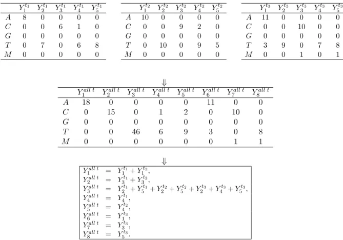
Table 2.2: Toy example of joining and preprocessing three 5×5 data matrices. The first few columns in the joint data matrix (second row) are the consolidation of columns with single nucleotide read in the sampled data panels (first row). The remaining columns of the joint data matrix are the copies of non-homogeneous reads of the sample (first row). The detail of the consolidation process is described in the panel in the third row.
2.3.1
Preprocess
Continuing with the toy example in Figure 2.2, the first step is to combine the datasets collected at different time points and consolidate the invariant read sites (Table 2.2). Assume that in the toy exampleJ = 5. The five possible reads are A, C, G, T, M, as in Table 2.1. The three small tables in the first row of Table 2.2 show the read counts obtained at time points t1, t2, and t3; the second row table shows the combined data of the first row
(Y1all t, Y2all t, Y3all tin the toy example). In particular,Y1all tin the joint data matrix (second row in Table 2.2) is formed by merging columns Yt1
1 and Y
t2
1 . Similarly, Y2all t, Y3all t are
formed from the sites that have a homogenous read ofC and T, respectively:
Y2all t=Yt1
3 +Y
t2
3 ,
Y3all t=Yt1
2 +Y
t1
5 +Y
t2
2 +Y
t2
5 +Y
t3
2 +Y
t3
4 +Y
t3
5 .
The following columns in the second row are
Y4all t=Yt1
4 , Y all t
5 =Y4t2, Y all t
6 =Y1t3, ...
The exact mapping is shown in the third row of the table. Note that this preporcessing step consolidates invariant sites and reduces the dimensionality of sequencing data without losing any significant information.
2.3.2
Processing
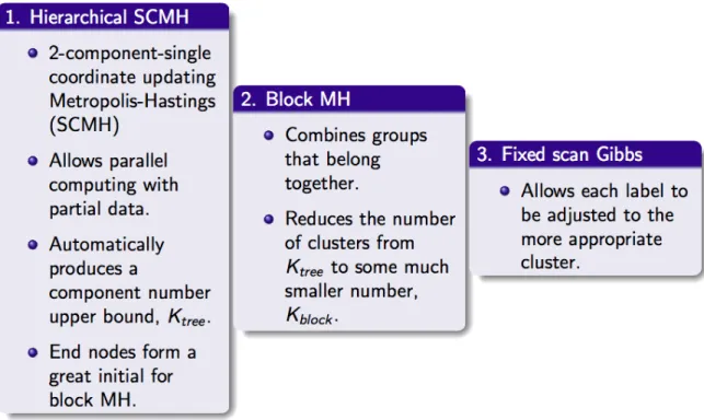
After preprocessing the read counts, a series of MCMC methods are implemented to cluster the geomic locations and obtain the assignment labels c0is(Figure 2.3).
The first step is a “top down” hierarchical clustering with 2-means initial states (hierar-chical SCMH) based on a two-component Single Coordinate updating Metropolis Hastings
Figure 2.3: Three steps clustering procedure. It automatically produces an upper bound fromK, assigns cluster labels to genomic sites at each time point, and allows parallel computing.
The divisive hierarichical clustering model allows us to avoid choosing a K, number of the mixture components. The total number of leaf nodes in the tree forms a reasonable upper bound for the number of mixture components regarding the entire joint data matrix. With sufficient number of observations at each site, mi (n.b. most sequencing data have
hundreds to thousands of sequencing reads), the Metropolis-Hasting splitting algorithm clusters correctly with probability one. This result is a direct consequence of the following theorem:
Theorem 2.1. Suppose thatY = [Y1, Y2],Y1 and Y2 areJ×1 random read count vectors.
J ∈ {2,3,4,· · · }. Further assume that Yi|ci,Pindep∼ Multinomial(mi;Pci), for i= 1,2.
If c1 =c2 = 1 andmi’s are sufficiently large, then the marginal posterior likelihood ratio of
assigning different labels over current state goes to zero almost surely,
i.e. LR= π(c1 = 1, c2 = 2|Y) π(c1 = 1, c2 = 1|Y)
→0, a.s.
Most genomes are lengthy, which results in high dimensional data. Direct application of multiple mixture component MCMC methods to this high dimensional data quickly becomes infeasible. Our hierarchical tree model enables efficient computing on this high dimesionality data. After the first split (at the root node) only a portion–typically only a small portion–of the original data set is analyze at a time. With this reduced input size, each Markov chain converges much faster. At the root node, although the entire joint sequence is used, there are only two possible values for each assignment label. Thus the Markov chain typically reaches convergence inexpensively. The hierarchical SCMH step is also easily parallelized for high performance computing systems. As a result, we have an efficient clustering procedure that automatically produces a component number upper bound and initial assignments for the block MH step.
In practice, the MCMC tree usually splits the data into too many groups. The block MH step, however, allows clusters to combine. The binary hierarchical clustering process therefore does not require the true number of components to be representable by binary clusters. The shrinkage property of the marginal distribution (2.1) favors combining leaf nodes that belong to the same group. As a result of this natural penalty on non-empty groups, the number of distinct groups at the end of the block MH step is almost always much smaller than the total leaf number in the hierarchical tree. The block MH step in essence tunes the assignments for each genome site and reduces the total number of mixture components. As shown later in Section 2.4, our clustering algorithm with only the first two steps (hierarchical SCMH & block MH) produces reasonable results with slightly higher error rate, compared to the full algorithm.
Occasionally a few indices in some end nodes can be misplaced in the tree splitting step. Because all the indices in each leaf node are kept in the same cluster throughout the block MH process, those position indices do not get a chance to be moved to a different cluster. We solve this by adding a fixed scan Gibbs sampler step, Gibbs, that can modify the assignments for individual indices and move them to more appropriate clusters.
mixture components K is provided. Furthermore, one must choose such a K ad hoc and risk either having a small mixture number that always misgroups elements from multiple true clusters together or risk having a large mixture number that might make computation infeasible. Further, most sequencing data sets are large. Direct Gibbs sampler might be infeasible even with a small K. Because the hierarchical SCMH step enables parallel computing and the block MH step works with a dataset of smaller dimension than the original, the computational cost is much lower in comparison to direct MCMC approaches. In the simulation study section (Section 2.4), we will compare the result and computation time using our three-step clustering approach to a direct Gibbs sampler with several choices of K, including the truth. We will show that our clustering is much more efficient, it outperforms the direct Gibbs sampler given the true K.
Alternatively, one can apply a Dirichlet process model to the joint dataset. A Dirichlet process model can be viewed as a Dirichlet mixture model with infinite number of compo-nents. With this framework, the point when cluster number stops growing depends heavily on the shrinkage power of the prior. Hence for a Dirichlet process model to work a more careful choice of prior is required. Intuitively, the computational time for the Dirichlet process is at best as good as a direct Gibbs sampler with the true K and a good initial state.
2.3.3
Postprocess
After implementing the three steps: hierarchical SCMH, block MH, and Gibbs, we obtain T running sets of assignment labels for the joint data. By reversing the preprocessing step (illustrated in Table 2.2) each genome position gets an assignment label for each time point from each Gibbs result. The posterior distribution per genome position per time point can now be computed. For each positioni, we use the transformed Hellinger distance, Ht (Equation 2.5), to compare posterior distributions before and after treatment. Given two time pointstk1, tk2, a collection of Hellinger distance values are obtained from the clustering
result for each location i. We take the median of those distance values and denote it as Ht(πtk1
i , π tk2
statistic of the Hellinger distance between treated and non-treated times for location i is denoted as Ht(Di). Large values in Ht(Di) indicate evolutionary changes in the viral
genome. Those changes can be caused by the treatment or non-treatment related reasons, such as genetic drift and adaptation to the host. To distinguish between these potential causes of changes, we denote a summary statistic Ht(Ni) for the comparison between time
points without treatment.
Exact form of the statistics Ht(Di) and Ht(Ni) depends on the experimental design.
The basic idea is that, at genomic locationi,Ht(Di) is the minimum change between the
last treated time point and all pre-treatment times, while Ht(Ni) is the maximum change
among pairwise comparisons between untreated samples. At position i, ifHt(Di) is large,
the last sampled population after treatment is significantly different fromallsamples before treatment; if Ht(Ni) is large, some untreated sample is significantly different from some
other untreated sample.
Intuitively, if the nucleotide read count distribution at site i has been affected by the treatment, Ht(Di) shall be large, relative to Ht(Ni) and the comparisons for all the other
sites that are not affected by treatment. How large is large will be determined by thresh-olding. For any given cutoffd, we define the following three sets:
S1d = {i: Ht(Di)> d},
S2d = {i: Ht(Ni)> d & Ht(Ni)> Ht(Di)},
S3d = S1d\Sd2.
determined by the tipping point where the size of S2d starts to increase dramatically, as d decreases.
To illustrate the derivation ofHt(Di) andHt(Ni), we continue with the toy example. It
can be easily generalized to more than three time point collections, with duplicates, or with a treatment-control setup (see Sections 2.4 & 2.5). Return to the toy example (Figure 2.2), which shares the same experimental setup as the HIV-1 study in Section 2.5.1; the treatment is administrated after t2; by time t3 the viral population have completely responded (see
Figure 2.4).
t1
t3D
t2
+ Treatment
Toy Example / HIV
Figure 2.4: Illustration of the experimental setup the toy example and the HIV data. This setup includes two untreated populations (t1, t2) and one post-treatment population (t3D). Observations
are collected from each time point.
For each genome sitei, we compare its marginal posterior distributions (Eq 2.2) at time t1, t2, and t3D, denoted as πit1, πit2, πti3D, respectively, using the transformed Hellinger
distance (Eq 2.5). Taking the clustering results from parallel chains, for a site i, we may define the summary statisticsHt(Di) and Ht(Ni) as
Ht(Di) = min{Ht(πit1, πit3D), Ht(πti2, πit3D)}, Ht(Ni) =Ht(πit1, πit2), ∀i. (2.6)
If the change of read count distribution is caused by the treatment, the posterior distribution πt3D
i ought to be much different from π t1
i and π
t2
i . Consequently, both
Ht(πt1 i , π
t3D
i ) and Ht(π t2 i , π
t3D
i ) result in large values. Large Ht(Di) value guarantees that
both Ht(πt1 i , π
t3D
i ) and Ht(π t2 i , π
t3D
Depending on the noise level of the data, the boundary of noise and signal portions of the data can be approximated by the curvature of noise set size function as the cutoff d decreases. The size of S2d is a step function ofd. We suggest to plot the size ofS2d against a decreasing series of cutoffs. We approximate the curvature of the plot by looking at the total segment length of every consecutive ∆ number of steps. We then pick the point whose left ∆ steps minus its right ∆ steps is the largest as the optimal point. The default ∆ value is 3 in our program. Larger ∆ values lead to more coarse yet more robust approximation of the curvature. We also require a minimum length for the step on the left of the optimal point to guarantee that the noise set did not enlarge shortly after the value that is slightly greater than the cutoff. If the step on the left of the optimal point is shorter than the required minimum length, we move the optimal point to the left by one step and the check the length of the next step. The final threshold is chosen to be the optimal point shifted to the left by the minimum length. This default sets the minimum length to be half (α= 0.5) of the average length of the left ∆ steps. A largerαleads to a more conservative result while a smaller α corresponds to a more liberal result. Both ∆ and α = 0.5 are introduced to mathematically capture the boundary of noise and signal sections of the data. In practice, we suggest users to verify the output by examining the site count plot directly.
2.4
Simulation Study
In this section, we use simulations test our algorithm, with and without theGibbs modifi-cation step, and compare its efficiency with direct Gibbs samplers.
Consider the following experiment setup for a viral population with genome length 300 nucleotides and five possible nucelotides at each genome site: A, C, G, T, M (see Figure 2.5).
The simulation mimics the experiment which first samples the RNA data twice be-fore the administration of the treatment (t1, t2), then obtains a control group (t3) and a treatment group (t3D). For each genome site at time t1, t2, t3, the sequencing read count
t1
t2
t3 t3D
Control Treatment
+ Treatment Simulation
Figure 2.5: The experimental design used for the simulated test data. After two generations without treatment (t1, t2) the population is split into a control group t3 and a treatment group t3D. The treatment group is given a drug and allowed to evolve resistance to that drug for a
few generations. The before treatment, control group, and treatment populations are sampled and sequenced.
81 are generated from alternative multinomial distributions, while the rest follow the same multinomial distributions as other time points.
As discussed in Section??, we assume that the probability parameter for the nucleotide at each genomic location is sampled from a Dirichlet mixture model. For the sample without treatment, total 15 probability parameters, P1, P2,· · · , P15, are used to generate the five
possible reads: A, C, G, T, M. Five additional probability parameters, P16, P17,· · ·, P20,
are introduced to generate the treated population. The total number of mixture component for the joint dataset is therefore 20.
At each genomic location i, the corresponding summary statistics are Ht(Di) = min{Ht(πti1, π
t3D
i ), Ht(π t2 i , π
t3D i )}
Ht(Ni) = max{Ht(πit1, πit2), Ht(πit1, πit3), Ht(πit2, πit3)}
(2.7)
obtained using our method at two different choices ofα(α= 0.5,0.25). At either threshold, without or with Gibbs, both S1d and S3d have five elements; Sd2 is empty. It is clear that a wide range ofα parameter would produce different threshold, yet the same results here. The right two panels present the summary statisticsHt(Di) (small green circle) andHt(Ni)
(blue cross) at each genome position. The horizontal dashed and dotted lines correspond to the thresholds chosen in the left panels. Above the dashed line, five large red circles highlights the Ht(Di) corresponding to the signal sites in right panels. They show much
larger values than the rest and reveal clear separation between signals and noise. The potential set, noise set, and signal set are:
S1d0 ={1,21,41,61,81}, Sd0
2 =∅, S d0
3 =S1d0. (2.8)
Compared between without and with the Gibbs step, the inference results are equally good for this simulated dataset.
9 8 7 6 5 4 3
0
20
40
60
80
100
Test 1 (no Gibbs)
Threshold d
# of sites
signal
potential noise
α =0.5
α =0.25
0 50 100 150 200 250 300
0
2
4
6
8
10
Summary Stats (no Gibbs)
Genome site index
Ht
d0
Ht(Di) Ht(Ni) Signal
9 8 7 6 5 4 3
0
10
20
30
40
Test 1 (3 steps)
Threshold d
# of sites
signal
potential noise
α =0.5
α =0.25
0 50 100 150 200 250 300
0
2
4
6
8
10
Summary Stats (3 steps)
Genome site index
Ht
d0
Ht(Di) Ht(Ni) Signal
Figure 2.6: The result plots for Test 1 without (top) and with (bottom) the Gibbsstep. The left two panels show the number of elements of Sd
1, S2d, S3d as the threshold ddecreases with thresholds
indicated in dashed (α= 0.5) and dotted lines (α= 0.25); the right two panels are the summary statistics plots with correspond thresholds to the left. The small green circles and blue pluses are theHt(Di) values andHt(Ni) values, respectively. For genome siteithat belongs to the signal set,
itsHt(Di) value is highlighted in a large red circle. The five red circles on the top left correspond
to the true substitution sites: 1, 21, 41, 61, 81. There is a clear separation between signals and the rest of the sites.
Result Our method Direct Gibbs
w/Gibbs w/o Gibbs K = 20 K = 40 K = 60 K = 80
PR 100 97 99 100 100 100
FN 0 0 1 0 0 0
FP 0 3 0 0 0 0
FNP 0 0 0 0 0 0
Table 2.3: Result comparison of our method, Gibbs withK= 20, Gibbs withK= 40, and Gibbs withK= 60 using a variety of thresholds. PR, FN, FP, FNP are the number of tests with perfect results, only false negatives, only false positives, both false negatives and false positives, respectively. All methods show good results. TheGibbsstep improves the result over theblock MHstep alone.
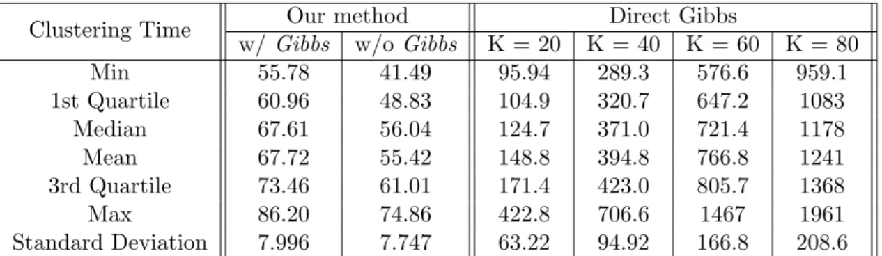
To assess the efficiency of our sequential MCMC algorithm, we also compared the clus-tering time (measured in CPU time) of the methods discussed in Table 2.3 for the 100 synthetic data sets (see Table 2.4). For each test, the reported time under our method was the waiting time for the processing step (with or withoutGibbs); the reported time for the direct Gibbs samplers was the time needed for one chain completing with corresponding K-means initial states. The CPU time is based on compute nodes including 122 blade servers, each with 8-cores 2.80 GHz Intel processors, 2×4M L2 cache (Model X5560), and 48GB memory for a total of 976 processing cores, two similar 8 core blades with 96 GB mem-ory, and three more blades with 192 GB memory and 24 total cores. Summaries including means and standard deviations of computing time are recored for each method. As shown below, our method takes only a fraction of the time needed for the direct Gibbs, even when the true K is given. The variation of clustering time among the 100 tests is also much smaller using our algorithm. AsK increases, the processing time for the direct Gibbs grows rapidly. It is worthy noted that the general computational issue with Gibbs sampler also affects the modification step in our algorithm. Our algorithm without theGibbs step does not suffer the same issue. At the price of slight higher error rate, it produces reasonable results promptly.
2.5
Real Data Analysis
Clustering Time Our method Direct Gibbs
w/Gibbs w/o Gibbs K = 20 K = 40 K = 60 K = 80
Min 55.78 41.49 95.94 289.3 576.6 959.1
1st Quartile 60.96 48.83 104.9 320.7 647.2 1083
Median 67.61 56.04 124.7 371.0 721.4 1178
Mean 67.72 55.42 148.8 394.8 766.8 1241
3rd Quartile 73.46 61.01 171.4 423.0 805.7 1368
Max 86.20 74.86 422.8 706.6 1467 1961
Standard Deviation 7.996 7.747 63.22 94.92 166.8 208.6
Table 2.4: Clustering time comparison in CPU time. For each test set, the corresponding process time of the direct Gibbs was that of a single Markov chain with K-means initial state for Gibbs sampler given a pre-chosen number of clusters. For our method, the corresponding process time records the total waiting time (in CPU time) needed for the processing step to finish 100 parallel Markov chains for each test set. The medians, means, and standard deviations here are from all 100 test sets. Our algorithm shows clear advantage in computational efficiency.
dataset produced by serially passaging the virus in kidney cells both in the presence and in the absence of an anti-viral drug.
2.5.1
Human immunodeficiency virus 1 (HIV-1)
As a ”positive control”, we applied our approach to an experimentally well characterized HIV-1 dataset (Jabara et al., 2011). Viral RNA was extracted from three longitudinal blood plasma samples taken from one individual infected with subtype B HIV-1, participating in a protease inhibitor (ritonavir) efficiency trial (Cameron et al., 1998). 454 sequencing was used to survey the genetic variation at the protease (pro) gene within the viral population. This population variation was surveyed twice, separated by six months, prior to ritonavir drug selection (t1, t2) and then once after the initiation of therapy (t3D). HIV-1 is known
to rapidly evolve resistance to ritonavir and several resistance mutations in the pro gene have already been identified and confirmed within vitro experiments. Thus, if our method is efficacious we should recover these same sites through our analysis.
The length of the protease gene is 297. As in the toy example, there are five possible reads and the corresponding Hellinger summary statistics are
Ht(Di) = min{Ht(πit1, π t3D
i ), Ht(π t2 i , π
t3D
i )}, Ht(Ni) =Ht(πit1, π t2
i ), i= 1,· · · ,297.
The inference results based on clustering without and with the Gibbs step are shown in the top and bottom panels of Figure 2.7 respectively. The left two panels set size plot of Sd1, S2d, S3d as the threshold d decreases (zoom-in); the right are the summary statistics plots. The thresholds according to two α parameter levels, α = 0.5 (dashed line) and α = 0.5 (dotted line), are plotted as well. In the summary statistics panels, the large red circles highlight the signal with default α(= 0,5). Looking at the trajectory of the S2dsize function in the top left panel, the default α appears to be too conservative, only site 245 was identified. The smaller α seems to be more appropriate, with which, three additional sites, 48, 55, 268, were added to the signal set. The two α levels considered in the full algorithm produce similar thresholds and the same inference result:
Sd0
1 ={48,55,243,245,250,264,268}, S d0
2 ={70,72,168,219,289}, S d0
3 =S
d0
1 . (2.10)
Due to the noise level and limited time points of this dataset, the clustering without the Gibbs produced more conservative results. In the detected signal set, sites 48, 55, 245, 250 268 correspond to known drug resistance mutations (Jabara et al., 2011). The other two sites identified, positions 243 and 264, both correspond to synonymous amino acid variation prior to treatment that disappeared post treatment. Meanwhile, the corresponding amino acids to sites 70, 72, 168, 219, 289, in the noise set S2d0, were identified as high variability in the study of genetic variation in the untreated environment (Jabara et al., 2011).
7 6 5 4
0
10
20
30
40
50
HIV1 (no Gibbs)
Threshold d
# of sites
signal
potential noise
α =0.5
α =0.25
0 50 100 150 200 250 300
0
2
4
6
8
Summary Stats (no Gibbs)
Genome site index
Ht
d0
Ht(Di) Ht(Ni) Signal
7 6 5 4
0
10
20
30
40
HIV1 (3 steps)
Threshold d
# of sites
signal
potential noise
α =0.5
α =0.25
0 50 100 150 200 250 300
0
2
4
6
8
Summary Stats (3 steps)
Genome site index Ht d0
Ht(Di) Ht(Ni) Signal
Figure 2.7: Results from the HIV-1 protease genome data set, without (top) and with (bottom)
theGibbsstep. The left panels show the sizes of setsSd
1, S2d, S3das the thresholdddecreases; the right
panels are the summary statistics plots with signal identified (with default parameters) highlighted in red circles. Without the modification step, the defaultαappears to be too conservative. For the full algorithm result, either choice ofαproduced the same inference result with seven signal sites: 48, 55, 243, 245, 250, 264, 26, and five noise sites: 70, 72, 168, 219, 289.
2.5.2
H1N1 Influenza A (IVA)
We applied our method to the whole-genome sequencing time series data of influenza A virus A/Brisbane/59/2007 strain (NIH Biodefencse and Emerging Infectious Research Resources Repository NIAID, NIH; NR-12282; lot 58550257). The data were collected from multiple passages in the presence and absence of an inhibitor of neuraminidase, oseltamivir, for a total of two biological replicates (E1 & E2) (see Figure 2.1). At the end of each passage, whole-genome high throughput sequencing data were collected. The read counts are unbalanced between the two experiments, as the first replicate, E1, consistently had more reads than the second one. There are four possible nucleotides: A, C, G, T, i.e.J = 4.
This IVA strain consists of 8 segments: PB2 (2313 nucleotides (nts)), PB1 (2301 nts), PA (2303 nts), HA (1775 nts), NP (1396 nts), NA (1426 nts), M1/2 (1005 nts), and NS1/2 (869 nts). To reduce computational intensity, we examine each segment per replicate separately. Within each duplicate, we analyze the control and treatment groups over selected time points simultaneously. In particular, we choose five time points: 1, 3, 9, 12, and the end (13 and 18 for E1 and E2, respectively). As the first three passages were shared across groups, we analyze total of 8 time-samples, three of which were treated, for each biological replicate. Denote the 8 collection times as t1, t2, t3, t4, t5, t3D, t4D, t5D. The summary statistics are
then formulated as
Ht(Di) = min{Ht(πit1, πit5D), Ht(πit2, πit5D)}
Ht(Ni) = max{Ht(πti1, π t2
i ), Ht(π t1 i , π
tj
i ), Ht(π t2 i , π
tj
i ), j= 3,4,5}
(2.11)
To allow additional response time for the drug, the comparisons tot3D and t4D are not
directly included inHt(Di).
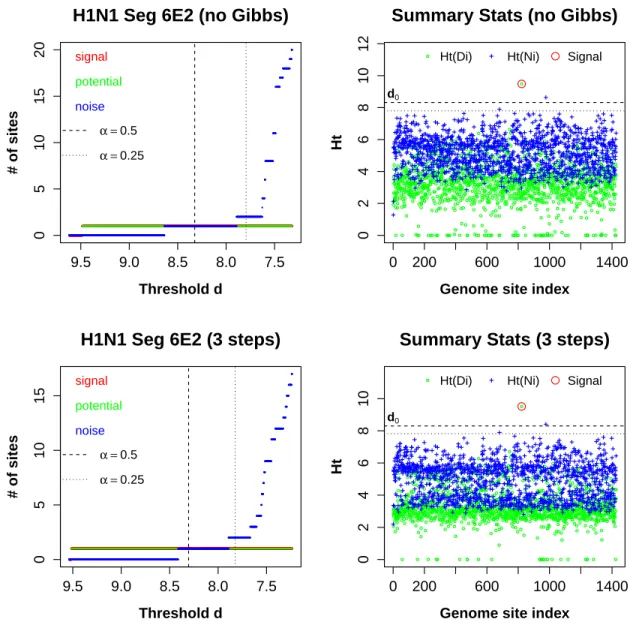
Taking segment 6 as an example, we analyzed both replicates simultaneously, without and with the Gibbs step. The result plots for E1 and E2 are presented in Figures 2.8 & 2.9, respectively. Both replicates revealed site 833 (S6-822). The clear separation between Ht(DS6−822) and the rest indicates that there is strong signal attributable to the treatment
for S6-822.
12 11 10 9 8
0
5
10
15
20
H1N1 Seg 6E1 (no Gibbs)
Threshold d
# of sites
signal
potential noise
α =0.5
α =0.25
0 200 600 1000 1400
0
5
10
15
Summary Stats (no Gibbs)
Genome site index
Ht
d0
Ht(Di) Ht(Ni) Signal
12 11 10 9 8
0
5
10
15
H1N1 Seg 6E1 (3 steps)
Threshold d
# of sites
signal
potential noise
α =0.5
α =0.25
0 200 600 1000 1400
0
2
4
6
8
10
14
Summary Stats (3 steps)
Genome site index
Ht
d0
Ht(Di) Ht(Ni) Signal
Figure 2.8: The results for H1N1 Seg6E1. Without (top panels) or with (bottom panels) the
Gibbs step, our algorithm identified one signal site, site 822 (S6-822). It corresponds to a known
oseltamivir-resistant mutation for H1N1. The inference result for H1N1 Seg6E1 is consistent even without theGibbsstep, and is robust to the choices ofαparameter.
9.5 9.0 8.5 8.0 7.5
0
5
10
15
20
H1N1 Seg 6E2 (no Gibbs)
Threshold d
# of sites
signal
potential noise
α =0.5
α =0.25
0 200 600 1000 1400
0
2
4
6
8
10
12
Summary Stats (no Gibbs)
Genome site index
Ht
d0
Ht(Di) Ht(Ni) Signal
9.5 9.0 8.5 8.0 7.5
0
5
10
15
H1N1 Seg 6E2 (3 steps)
Threshold d
# of sites
signal
potential noise
α =0.5
α =0.25
0 200 600 1000 1400
0
2
4
6
8
10
Summary Stats (3 steps)
Genome site index
Ht
d0
Ht(Di) Ht(Ni) Signal
Figure 2.9: The result plots for H1N1 Seg6E2. Similar to Seg6E1, without (top panels) and with (bottom panels) theGibbsstep, our algorithm identified site 822 (S6-822). The inference result for H1N1 Seg6E1 is consistent even without theGibbsstep, and is robust to the choices ofαparameter.
(Collins et al., 2008). The color tiles on the top of each panel indicates that the total read count at each time point varies.
Figure 2.10: H1N1 nucleotide read count proportion and total count at position S6-822. The top and bottom rows are for Replicate I and Replicate II, respectively; the left and right panels are for control and treatment groups, respectively. For the treated groups, there is a complete transition from C to T due to the drug. The color tiles on the top of each panel indicates the total read count at each time point.
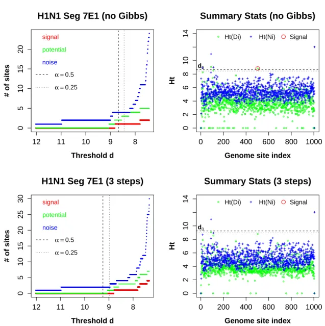
we are initially interested in substitution sites that are not replicate specific, we are only looking for signals observed in both biological replicates. The one red circle above threshold (top right panel of Figure 2.11) corresponds to S7-503. It appears to be a signal site based on E1, without the Gibbs. However, in Seg7E2, Ht(DS7−503) is below the threshold (top
12 11 10 9 8
0
5
10
15
20
H1N1 Seg 7E1 (no Gibbs)
Threshold d
# of sites
signal
potential noise
α =0.5
α =0.25
0 200 400 600 800 1000
0
2
4
6
8
10
14
Summary Stats (no Gibbs)
Genome site index
Ht
d0
Ht(Di) Ht(Ni) Signal
12 11 10 9 8
0
5
10
15
20
25
30
H1N1 Seg 7E1 (3 steps)
Threshold d
# of sites
signal
potential noise
α =0.5
α =0.25
0 200 400 600 800 1000
0
2
4
6
8
10
14
Summary Stats (3 steps)
Genome site index
Ht
d0
Ht(Di) Ht(Ni) Signal
Figure 2.11: The results for H1N1 Seg7E1. Without the Gibbs step (top panels), S7-503 was highlighted. However,Ht(DS7−503) does not exceed the threshold with the full algorithm(bottom
right panel). Site 91 showed large summary statistic valuesHt(NS7−91) &Ht(DS7−91) in both right
panels. The control statistic value for S7-1005 is alarmingly high. We suspect that is the result of low alignment quality at the tail of the segment. The inference result for H1N1 Seg7E1 is robust to the choices ofαparameter.
There is one site, S7-91, that consistently presented large Ht(Di) and Ht(Ni) values
13 12 11 10 9 8
0
5
10
15
20
H1N1 Seg 7E2 (no Gibbs)
Threshold d
# of sites
signal
potential noise
α =0.5
α =0.25
0 200 400 600 800 1000
0
5
10
15
Summary Stats (no Gibbs)
Genome site index
Ht
d0
Ht(Di) Ht(Ni) Signal
13 12 11 10 9 8
0
5
10
15
H1N1 Seg 7E2 (3 steps)
Threshold d
# of sites
signal
potential noise
α =0.5
α =0.25
0 200 400 600 800 1000
0
5
10
15
Summary Stats (3 steps)
Genome site index
Ht
d0
Ht(Di) Ht(Ni) Signal
Figure 2.12: The result plots for H1N1 Seg7E2. The inference result for H1N1 Seg7E2 is consistent even without theGibbsstep, and is robust to the choices ofαparameter. No site was identified as signal. Similar to Seg7E1,Ht(NS7−91) &Ht(DS7−91) exceeded the thresholds in both right panels.
A site on the tail part of the segment, S7-1004, showed large control statistic values.
captures the read type switch that is likely due to genetic drift or adaptation to the host cells–not the drug.
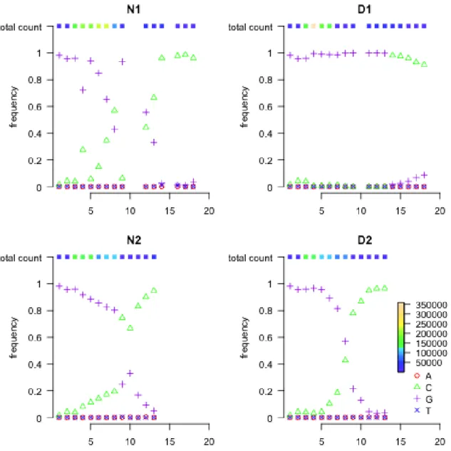
Figure 2.13: H1N1 nucleotide read count proportion and total count at position S7-91. All four panels show complete transversion from G to C.
standard Gibbs sampler, in which case, one may skip theGibbs step at the cost of a slightly higher error rate.
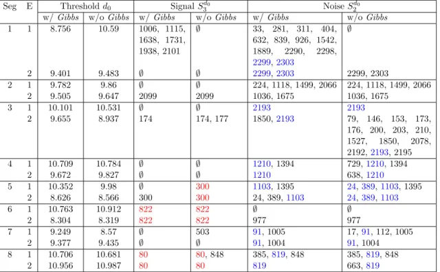
Seg E Thresholdd0 SignalS3d0 NoiseS
d0 2 w/Gibbs w/oGibbs w/Gibbs w/oGibbs w/Gibbs w/oGibbs 1 1 8.756 10.59 1006, 1115,
1638, 1731, 1938, 2101
∅ 33, 281, 311, 404, 632, 839, 926, 1542, 1889, 2290, 2298, 2299,2303
∅
2 9.401 9.483 ∅ ∅ 2299,2303 2299, 2303
2 1 9.782 9.86 ∅ ∅ 224, 1118, 1499, 2066 224, 1118, 1499, 2066
2 9.505 9.647 2099 2099 1036, 1675 1036, 1675
3 1 10.101 10.531 ∅ ∅ 2193 2193
2 9.655 8.937 174 174, 177 1850,2193 79, 146, 153, 173,
176, 200, 203, 210, 1527, 1850, 2078, 2192,2193, 2195
4 1 10.709 10.784 ∅ ∅ 1210, 1394 729,1210, 1394
2 9.672 9.827 ∅ ∅ 1210 638,1210
5 1 10.352 9.98 ∅ 300 1103, 1395 24,389,1103, 1395
2 8.626 8.566 300 300 24, 389,1103 24,389,1103
6 1 10.763 10.912 822 822 ∅ ∅
2 8.304 8.319 822 822 977 977
7 1 9.249 8.57 ∅ 503 91, 1005 17,91, 112, 1005
2 9.377 9.435 ∅ ∅ 91, 1004 91, 1004
8 1 10.706 10.681 80 80, 848 385,819, 848 385,819, 848
2 10.956 10.987 80 80 819 663,819
Table 2.5: Result derived using Passages 1, 3, 9, 12, and the end time point. The table provides the thresholds and corresponding signal & noise sets for each segment according to each biological replicate with and without the Gibbs step. The sites identified as signal in both experiments are highlighted in red, the ones identified as noise in both experiments are highlighted in blue. The modification step took much more time comparing to the first two steps. The w/Gibbsresults was not finished for Seg1E1 and Seg2E1 in four weeks time with standard Gibbs. In comparison, the algorithm with or without the modification step produced similar final result after cross check the replicates.
Table 2.5. All of our findings are supported by the raw nucleotide read proportion plots (See Figures 2.10, 2.21, 2.22, 2.23, 2.24, 2.25, 2.28, 2.13, 2.29).
rate, however, with multiple time points and replicates, the clustering result without the Gibbs leads to similar inference conclusion as basing on the full algorithm. When drawing inference without the modification step, we advise to double check the shift parameter α, as the default setting might not be the best for capturing the curvature of noise set size function.
We required that a ”true” site be one that showed the same evolutionary behavior in both replicates. This approach is conservative as it requires that the same evolutionary path is taken by both viral populations, which may not necessarily be true. While at least two sites–including a known resistance variant–meet this strict criterion, there are several ”signal” sites in each replicate that do not. These are potentially replicate specific adaptations. Moreover, it is possible the same amino acid can evolve through different nucleotide substitutions. For example, on segment 2 positions 31 and 32 evolved in Seg2E1 and Seg2E2 respectively. These neighboring changes both affect the amino acid lysine coded for by the 10th codon of the protein. Similar pattern is seen at sites 1004, 1005 on segment 7.
The first 12 passages of the dataset (Figure 2.14) were analyzed by Foll et al. from a population genetics and structural perspective (Foll et al., 2014). According to that study, the following sites are identified drug resistant: S2-32, S3-2193, S4-47, S4-1394, S6-581, S6-822, S7-146, S8-819; the sites with evolutionary changes without treatment are S2-1118, S4-1394, S5-1103, S5-1395.
For a fairer comparison to Foll et al, we applied our method to the joint data from Passages 1, 3, 9, 12 for both the control and treatment groups, i.e. t1, t2, t3, t4, t3D, t4D.
The summary statistics used are
Ht(Di) = min{Ht(πti1, πit4D), Ht(πit2, πti4D)}
Ht(Ni) = max{Ht(πti1, π t2
i ), Ht(π t1 i , π
tj
i ), Ht(π t2 i , π
tj
i ), j= 3,4}
(2.12)
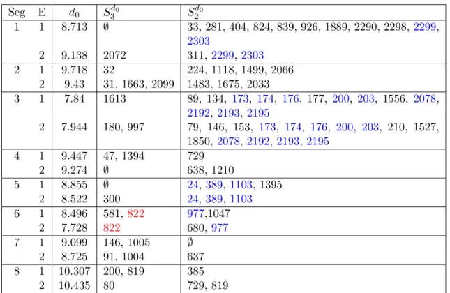
The result from each biological replicate is shown in Table 2.6. Here we used the default parameters, ∆ = 3, α= 0.5, and the summary results are for without theGibbs step.
Seg E d0 S3d0 S d0
2
1 1 8.713 ∅ 33, 281, 404, 824, 839, 926, 1889, 2290, 2298,2299, 2303
2 9.138 2072 311, 2299,2303
2 1 9.718 32 224, 1118, 1499, 2066
2 9.43 31, 1663, 2099 1483, 1675, 2033
3 1 7.84 1613 89, 134, 173, 174, 176, 177, 200, 203, 1556, 2078, 2192,2193, 2195
2 7.944 180, 997 79, 146, 153, 173, 174, 176, 200, 203, 210, 1527, 1850, 2078, 2192,2193,2195
4 1 9.447 47, 1394 729
2 9.274 ∅ 638, 1210
5 1 8.855 ∅ 24,389,1103, 1395
2 8.522 300 24,389,1103
6 1 8.496 581,822 977,1047
2 7.728 822 680, 977
7 1 9.099 146, 1005 ∅
2 8.725 91, 1004 637
8 1 10.307 200, 819 385
2 10.435 80 729, 819
1
2
3
4 4
4 4
12 12
12 12
Replicate I Replicate II
MDCK
Control Treatment Control Treatment + Treatment + Treatment
Figure 2.14: Only the first 12 passages were used in Foll et al (Foll et al., 2014). The complete dataset includes two biological replicates with one control group and one treatment group. Each ovals presents a passage. The colors white and red indicate absence and presence of the inhibitor. The sizes of the ovals indicate the average total read count per genome site. Note that the first replicate have much larger total reads than the second.
S2-32 sites of our analysis are treated as one). Several other sites, S1-2299, S2-2303, S3-173,174,176,200,203, 2078,2192,2193,2195, S5-24,389,1103, S6-977, were identified as loca-tions with evolutionary changes not due to the treatment.
Intriguingly, most sites identified in Foll et al. (Table 2.6) appear in our analysis to only have signal in the first biological replicate. The exception, S6-822, has a strong signal in both replicates and regardless of end point generation analyzed (2.10). We speculate that the lack of consistent signal/false signal coming from the other sites is caused by the lower average read count per site for the second replicate compare to the first. The population genetic approach used in Foll et al. appears to be heavily influenced by the first replicate. This leads us to postulate that their result is adversely affected by the large imbalance in counts.
Foll et al. Thus our previous analysis, which included the last time point collection, is likely more reliable for the identification of substitution sites.
2.6
Discussion
We introduce a Dirichlet mixture model for detecting and clustering changes in allele fre-quencies in DNA or RNA sequence data from a population sampled at different time points. This annotation free approach is particularly useful for RNA viruses and other organisms where the secondary structure of the RNA can influence evolution in ways not predicted by standard molecular evolutionary analysis methods.
To identify significant changes in allele frequency, our clustering algorithm uses a com-bination of a hierarchical divisive clustering tree (hierarchical SCMH), a block Metropolis-Hasting (block MH), and a fixed scan Gibbs sampler (Gibbs) procedures. This approach does not require a prior distribution on the number of mixture components. The hier-archical SCMH step automatically produces an upper bound for the number of mixture components, K, and fine clusters for the block MH step. The hierarchical tree structure enables parallel computing and overcomes the computational difficulties any direct Markov chain Monte Carlo method presents. The block MH step improves the upper bound for K and combines similar clusters. Last but not least, the Gibbs step modifies the clustering result. The threshold for identifying substitution sites is derived based on the posterior dis-tribution comparison for the time collections without treatment. It is chosen by examining the curvature in the graph of the number of members in the noise set instead of selecting an ad hoccutoff.
The last cluster step of our algorithm, theGibbs, can take a long time if the consolidated dataset is still very large. One may choose to skip this modification step at the price of a slightly higher error rate. It is advised to check the set size function plot and determine if the default parameters are appropriate.
As a positive control, we applied our method to a well described HIV-1 dataset. With minimal assumptions on gene annotation or the coding nature of the substitution, we suc-cessfully identified known drug resistance alleles previously reported (Jabara et al., 2011) and a list of sites with significant allelic changes within untreated population.
In the IVA dataset that motivated this study, we analyzed multiple time points and treatment-control simultaneously. We identified two sites, S6-822 & S8-80, with strong evi-dence of evolution in response to inhibitor treatment and six locations with high variability not due to the inhibitor. We compared our findings to a previous analysis of the same dataset based on a population genetic approach. Noticing that most of the sites identified using the latter method only appear in the biological replicate with larger sample size, we suspect that the population genetic based approach is biased due to this imbalance. Our algorithm performs analysis on each biological replicate individually first and then aggre-gate the results across replicates. Therefore, our inference technique is not sensitive to the unbalanced nature of the data.
In this chapter we have applied our method to high-through put sequencing nucleotide read count data. It can also be applied to other count data, such as amino acids. As the model requires minimum assumption, it can be broadly applied. For example, this approach can be used to identify evolved sites in non-coding regions of the genome such as the regulator regions of genes or in RNA genes such as ribosomal RNA and other long non-coding RNAs.
2.7
Appendix
2.7.1
Proof of Theorem 2.1
Suppose there are only two genome positions to be clustered, Y = [Y1, Y2]. If they share
is one when the numbers of observations at the two sites m1 and m2 are large. Fix a
J ∈ {2,3,4,· · · }. Without loss of generality, assume c1 = c2 = 1, and then the marginal
posterior likelihood ratio of splitting the two over current state on the log scale is the following:
LR = log(π(c1= 1, c2 = 2|Y))−log(π(c1 = 1, c2= 1|Y))
=
J
X
j=1
h
log Γ(y1j+J−2) + log Γ(yj2+J−2)i−log Γ(m1+J−1)−log Γ(m2+J−1)
−
J
X
j=1
log Γ(y1j+y2j+J−2) + log Γ(m1+m2+J−1)
Claim: LR−→ −∞ a.s.
Proof. Recall that Stirling’s formula provides the following approximation:
log Γ(z)≈ 1
2log(2π)− 1
2logz+zlogz−z Therefore, LR ≈ J X j=1 1
2log(2π)− 1 2(y
j 1+J
−2)−1
2(y
j 2+J
−2) +1
2(y
j 1+y
j 2+J
−2) + (yj 1+J
−2) log(yj 1+J
−2)
+(yj2+J−2) log(y2j+J−2)−(y1j+yj2+J−2) log(y1j+y2j+J−2)−J−2
i − 1
2log(2π) +1
2log(m1+J
−1) + 1
2log(m2+J
−1)−1
2log(m1+m2+J
−1)−(m
1+J−1) log(m1+J−1)
−(m2+J−1) log(m2+J−1) + (m1+m2+J−1) log(m1+m2+J−1) +J−1
= J −1
2 log(2π) +
J
X
j=1
yj1+J−2−1 2
log(yj1+J−2) +
yj2+J−2−1 2
log(yj2+J−2)
−
y1j+y2j+J−2−1 2
log(y1j+y2j+J−2)
+
m1+m2+J−1−
1 2
log(m1+m2+J−1)
−
m1+J−1−
1 2
log(m1+J−1)−
m2+J−1−
1 2
log(m2+J−1)
Under null hypothesis that Y1 and Y2 follow the same distribution, i.e. they share