NON-GAUSSIAN SEMI-STABLE DISTRIBUTIONS AND THEIR STATISTICAL APPLICATIONS
Ritwik Chaudhuri
A dissertation submitted to the faculty of the University of North Carolina at Chapel Hill in partial fulfillment of the requirements for the degree of Doctor of
Philosophy in the Department of Statistics and Operations Research in the University of North Carolina at Chapel Hill
Chapel Hill 2014
ABSTRACT
RITWIK CHAUDHURI: NON-GAUSSIAN SEMI-STABLE DISTRIBUTIONS AND THEIR STATISTICAL APPLICATIONS
(Under the direction of Vladas Pipiras)
The dissertation is motivated by problems arising in modern communication net-works such as the Internet. Over these netnet-works, information is sent in the form of data packets which are further grouped into flows. For example, a flow can be asso-ciated with a certain (document, music, movie or other) file. Knowing the structure of flows is of great interest to network operators and networking researchers. One quantity of particular interest is the distribution of flow sizes (the number of packets in a flow).
Each packet carries information on the flow it belongs to. Hence, examining all packets allows reconstructing and studying the associated flows. Examining all pack-ets, however, is becoming cumbersome due to the ever increasing amount of data and processing costs. To overcome these issues, packet sampling has become prevalent. One common sampling scheme is probabilistic sampling wherein each packet is sam-pled independently and with the same probability. The basic problem then becomes inference of the characteristics of original flows (e.g. the flow size distribution) from sampled packets (forming sampled flows).
suitable and restrictive assumptions, the estimator has been known to be asymptot-ically normal. Going beyond these assumptions, it is shown in the dissertation that the estimator can be asymptotically semi-stable.
To achieve this goal, the domains of attraction of semi-stable distributions are reexamined here. As a main theoretical contribution, general, sufficient and practi-cal conditions are provided for a distribution to be in the domain of attraction of a semi-stable distribution. They lead to practical conditions for the aforementioned nonparametric estimator to be attracted to a semi-stable law. Examples of proba-bility distributions and illustrations of the main results are provided throughout the dissertation. One practical consequence of the results is a confidence interval for the distribution of flow sizes, based on critical values of semi-stable distributions.
Semi-stable distributions do not have closed forms in general. In order to compute their critical values, numerical calculation of semi-stable densities is also considered in the dissertation. This is carried out by using a celebrated method of Joseph Abate and Ward Whitt, allowing numerical calculation of a density given its characteristic function (Laplace transform). The code implementing the method for semi-stable densities is included.
ACKNOWLEDGEMENTS
I wish to express my sincerest gratitude to my advisor Prof. Vladas Pipiras. He introduced me to the topic of heavy-tailed distributions and without his constant support, encouragement and invaluable insights this work would not have been pos-sible. I thank him for his constant support and patience with me and teaching me the importance of hard work in every walk of life. I thank him for helping me whenever I needed it. I feel grateful and very fortunate to have him as my mentor and the lessons that I learned through this journey will stay with me for the rest of my life. I will take this opportunity to specially thank Prof. Amarjit Budhiraja for teaching me Measure Theory in my first semester at UNC Chapel Hill. I learnt a lot about proba-bility through this class. My special thanks goes to Prof. Shankar Bhamidi for giving me honest suggestions whenever I needed it. He motivated me a lot through every discussion we had. I also thank Prof. Amarjit Budhiraja, Prof. Shankar Bhamidi, Prof. Chuanshu Ji and Prof. Andrew Nobel for being members of my dissertation committee and providing many useful comments.
TABLE OF CONTENTS
LIST OF TABLES . . . ix
LIST OF FIGURES . . . x
LIST OF ABBREVIATIONS AND SYMBOLS . . . xi
CHAPTER 1: INTRODUCTION . . . 1
1.1 Motivation . . . 1
1.2 Structure of dissertation and main results . . . 5
CHAPTER 2: SEMI-STABLE DISTRIBUTIONS . . . 8
2.1 Definitions and domains of attractions . . . 8
2.2 Numerical calculation of densities . . . 15
2.3 Semi-stable densities . . . 18
CHAPTER 3: SEMI-STABLE DOMAINS OF ATTRACTION . . . . 30
3.1 General results . . . 30
3.2 Special case and numerical illustrations . . . 61
CHAPTER 4: APPLICATION TO SAMPLING . . . 68
4.1 General results . . . 68
4.2 Examples . . . 71
4.3 Performance of confidence intervals . . . 76
A APPENDIX A: AUXILIARY RESULTS AND CODE . . . 84
A.1 Auxiliary results . . . 84
A.2 Code for numerical calculation . . . 89
LIST OF TABLES
LIST OF FIGURES
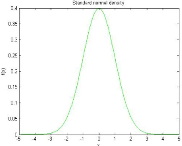
2.1 Plot of the standard normal distribution. . . 17
2.2 Stable density with α= 1.2,c= 1, β = 1. . . 19
2.3 Plot of actual stable density withα= 1.2,c= 1, β = 1. . . 20
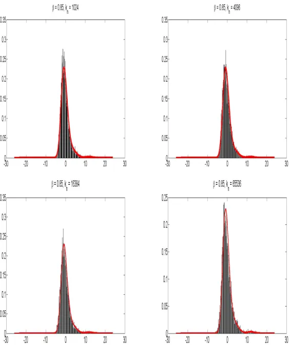
2.4 The empirical histogram against the actual density when β = 0.85. . 25
2.5 The empirical histogram against the actual density when β = 0.9. . . 26
2.6 The empirical histogram against the actual density when β = 0.95. . 27
2.7 The empirical histogram against the actual density when β = 1.05. . 28
2.8 The empirical histogram against the actual density when β = 1.1. . . 29
3.1 Plot of g0(y),g1(y) andg2(y). . . 36
3.2 The empirical histogram against the actual density. . . 66
3.3 The empirical histogram against the actual density. . . 67
LIST OF ABBREVIATIONS AND SYMBOLS
N Set of natural numbers
N0 Set of non-negative integers
R Set of real numbers
R+ Set of positive real numbers
Z Set of integers
[x] Largest integer smaller than or equal to x dxe Smallest integer larger than or equal x dxe
CHAPTER 1: INTRODUCTION
We describe here the motivation behind this dissertation (Section 1.1), and outline its structure with main result (Section 1.2).
1.1 Motivation
LetW, Wi,i= 1,2, . . . , N, be i.i.d. integer-valued random variables with the
prob-ability mass function (p.m.f.) fW(w), w ≥ 1. Let also Bin(n, q) denote a binomial
distribution with parameters n ≥ 1, q ∈(0,1). Consider random variables Wq, Wq,i,
i= 1,2, . . . , N, obtained fromW, Wi,i= 1,2, . . . , N, through the relationshipsWq =
Bin(W, q) and Wq,i = Bin(Wi, q), i= 1,2, . . . , N (independently across i). Note that
Wq takes values in 0,1,2, . . . , W. Let the probability mass function ofWq befWq(s),
s≥0. The basic interpretation of Wq is as follows. If an object consists ofW points
(a finite point process) and each point is sampled with a probability q, then the number of sampled points is Wq = Bin(W, q).
One application of the above setting arises in modern communication networks. A finite point process (an object) is associated with the so-called packet flow (and a point is associated with a single packet). Sampling is used in order to reduce the amount of data being collected and processed. One basic problem that has attracted much attention recently is the inference offW from the observed sampled data Wq,i,
i = 1,2, . . . , N (in principle, Wq,i = 0 is not observed directly, but the inference
about the number of timesWq,i = 0 is made through other means). See, for example,
We are interested in this dissertation in some statistical properties of a nonpara-metric estimator of fW(w), introduced in Hohn and Veitch [16] and also considered
in Antunes and Pipiras [2]. We first briefly outline how the estimator is derived. Estimation of fW(w) is based on a theoretical inversion of the relation
fWq(s) =
∞ X
w=s
P(Wq=s|W =w)P(W =w) =
∞ X w=s w s
qs(1−q)w−sfW(w), s≥0.
(1.1.1) In terms of the moment generating functionsGWq(z) =
P∞
s=0zsfWq(s) andGW(z) =
P∞
w=1zwfW(w), the relation (1.1.1) can be written as GWq(z) =GW(zq+ 1−q). By
changing the variables zq+ 1−q = x, one has GW(x) = GWq(q−1x−q−1(1−q))
which has the earlier form but with q replaced by q−1(and z replaced by x). This suggests that (1.1.1) can be inverted as
fW(w) =
∞ X s=w s w
(q−1)w(1−q−1)s−wfWq(s)
= ∞ X s=w s w
(−1)s−w
qs (1−q) s−wf
Wq(s), w≥1. (1.1.2)
Antunes and Pipiras [2], Proposition 4.1, showed that the inversion relation (1.1.2) holds when ∞ X s=n s n
(1−q)s−n
qs fWq(s) =
∞ X w=n w n
2w−n(1−q)w−nfW(w)<∞, n ≥1. (1.1.3)
Observe that (1.1.3) always holds when q ∈ (0.5,1). But when q ∈ (0,0.5], the finiteness of the above expression depends on the behavior of fW(w) as w→ ∞. We
In view of (1.1.2), a natural nonparametric estimator of fW is
b
fW(w) =
∞ X
s=w
s w
(−1)s−w
qs (1−q) s−w
b
fWq(s), w≥1, (1.1.4)
where
b
fWq(s) =
1 N
N
X
i=1
1{Wq,i=s}, s≥0, (1.1.5)
is the empirical p.m.f. of fWq, and 1A denotes the indicator function of an event A.
Note that, by using (1.1.4) and (1.1.2),
√
N(fbW(w)−fW(w)) =
∞ X
s=w
s w
(−1)s−w
qs (1−q) s−w√
N(fbWq(s)−fWq(s)). (1.1.6)
Since
{√N(fbWq(s)−fWq(s))}∞s=0
d
−
→ {ξ(s)}∞s=0, (1.1.7)
where {ξ(s)}∞s=0 is a Gaussian process with zero mean and covariance structure
E(ξ(s1)ξ(s2)) = fWq(s1)1{s1=s2}−fWq(s1)fWq(s2),
one may naturally expect that under suitable assumptions, (1.1.6) is asymptotically normal in the sense that
{√N(fbW(w)−fW(w))}∞w=1 d
−
→ {S(ξ)w}∞w=1, (1.1.8)
showed that (1.1.8) holds indeed if Rq,w <∞, w≥1, where
Rq,w =
∞ X s=w s w 2
(1−q)2(s−w)
q2s fWq(s)
=
∞ X
i=w
fW(i)(1−q)i−2w
i w i X s=w s w
i−w s−w
(q−1−1)s. (1.1.9)
We are interested infbW(w) when the conditionRq,w<∞, w ≥1, is not satisfied.
In fact, such a situation is expected with many distributions. For example, we show in Section 3.2 (Chapter 3) below that if fW(w) = (1−c)cw−1, w≥ 1, is a geometric
distribution with parameter c∈(0,1), then the distribution of fWq(s) is given by
fWq(s) =
(1−q)(1−c)
1−c(1−q) , if s = 0, 1
cc s
q(1−cq), if s ≥1,
(1.1.10)
where cq = 1−c(1cq−q). Moreover, the condition Rq,w <∞ holds if and only ifc < 1−qq
(see Section 3.2). Thus, for example, we are interested what happens with fbW(w)
when Wq has p.m.f. given by (1.1.10) with c≥ 1−qq.
To understand what happens when Rq,w = ∞, observe from (1.1.4) and (1.1.5)
that fbW(w) can also be written as
b
fW(w) =
1 N
N
X
i=1
Xi, (1.1.11)
where Xi, i= 1,2, . . . , N, are i.i.d. random variables defined as
Xi =
Wq,i
w
(−1)Wq,i−w
qWq,i (1−q) Wq,i−w
Focus on the key term (1−q)Wq,i
qWq,i = (q
−1−1)Wq,i entering (1.1.12). For example, when
W is geometric with parameterc,Wq,i has p.m.f. in (1.1.10). One then expects that
P((q−1−1)Wq,i > x) = P
Wq,i >
logx log(q−1−1)
≈ 1cc logx
log(q−1−1)
q =
1 cx
−α, (1.1.13)
where α = logc −1
q
log(q−1−1). This suggests that the distribution of Xi, i = 1,2, . . . , N, has
heavy tail and that the estimatorfbW(w) is asymptotically non-Gaussian stable when
α < 2. In fact, the story turns out to be more complex. Because of the discrete nature ofWq,i, the relation (1.1.13) does not hold in the asymptotic sense asx→ ∞.
An appropriate setting in this case involves the so-called semi-stable laws. In the semi-stable context, moreover, the convergence of (1.1.11) is expected only along subsequences of N.
Semi-stable laws have been studied quite extensively (see Section 2.1 for refer-ences). In particular, necessary and sufficient conditions are known for a distribution to be attracted to a semi-stable law (see Theorem 2.1.1 below). Verifying whether the distribution of (1.1.12) satisfies these conditions for a large class of p.m.f.’sfWq,
how-ever, turns out to be highly nontrivial. Much of this dissertation, in fact, concerns this problem. We identify a large class of p.m.f.’s, including (1.1.10), for which the dis-tribution Xi satisfies the sufficient (and necessary) conditions and hence is attracted
to a semi-stable law. We also study what this result means for the nonparametric estimator fbW(w).
1.2 Structure of dissertation and main results
properties of semi-stable distributions. We also provide known necessary and suffi-cient conditions for a distribution to be in the domain of attraction of a semi-stable distribution (Theorem 2.1.1).
For later applications, we will need to have critical values for semi-stable distribu-tions. The distribution function and the density of a semi-stable distribution are not available in closed form (except special cases) but its Laplace transformation is. In Section 2.2, we recall a popular method of Abate and Whitt [1] to calculate numeri-cally the density of a distribution given its Laplace transform. Numerical illustrations of the method applied to semi-stable laws can be found in Section 2.3.
In Section 2.3, we also evaluate numerically how well a semi-stable law approx-imates partial sums in its domain of attraction. Our findings here are that the goodness of the approximation very much depends on a parameter involved in the convergence result (more specifically the constant c in (2.1.5) below) with the per-formance degrading as the parameter increases.
Chapter 3 concerns the domains of attraction of semi-stable distributions. Though necessary and sufficient conditions for a distribution to be in the domain of attrac-tion are available (and recalled in Secattrac-tion 2.1 as indicated above), verifying those conditions is quite nontrivial in general. In Section 3.1, we provide a large family of distributions which satisfy these conditions and hence are attracted to semi-stable law (Theorem 3.1.1 and Corollary 3.1.2). The proof of the main result (Theorem 3.1.1) is quite lengthy. The form of the family is motivated by applications to sampling.
(Proposition 3.1.2). These results are important for practical applications, as in the case of sampling of finite point processes.
In Section 3.2, we consider a concrete example of a distribution from the derived family attracted to a semi-stable law. We also study numerically the goodness of approximation (of a partial sum by the limit semi-stable law) in finite samples.
In Chapter 4 and Section 4.1, in particular, we return to the sampling framework described in Section 1.1 and are interested in the asymptotics of the nonparametric estimator fW(w) in (1.1.4) of the p.m.f. fW(w) of the number of points in a finite
point process. Under suitable assumptions and by using the results of Chapter 3 we conclude thatfbW(w) can be asymptotically semi-stable (Theorem 4.1.1). This result
can be used to construct confidence intervals for fW(w) (Proposition 4.1.1).
In Section 4.2, we illustrate the results of Section 4.1 with several concrete exam-ples of p.m.f. fW(w). In the first example, W follows a geometric distribution, and
in the second example, W follows a negative binomial distribution.
In Chapter 5, we discuss several open problems and future directions.
CHAPTER 2: SEMI-STABLE DISTRIBUTIONS
This chapter concerns semi-stable distributions. Basic facts about semi-stable distributions and known results on their domains of attraction are recalled in Section 2.1. The Abate and Whitt [1] method for calculating numerically a density function is described in Section 2.2, and it is applied to semi-stable distributions in Section 2.3.
2.1 Definitions and domains of attractions
One way to characterize a semi-stable distribution is through its characteristic function (Maejima [20]).
Definition 2.1.1. A probability distribution µ on R (or a random variable with distribution µ) is called semi-stable if there exist r, b∈(0,1) and c∈R such that
b
µ(θ)r =µ(bθ)eb icθ, for all θ∈R, (2.1.1)
and µ(θ)b 6= 0, for all θ ∈R, where
b
µ(θ) =
Z
R
eiθxµ(dx)
denotes the characteristic function ofµ.
part with L´evy measure characterized by (distribution) functions
L(x) = ML(x)
|x|α , x <0, R(x) =−
MR(x)
xα , x >0, (2.1.2)
whereα∈(0,2),ML(c
1
αx) =ML(x) whenx <0, andMR(c
1
αx) =MR(x) whenx >0,
for somec >0. The functionsMLandMRare thus periodic with multiplicative period
cα1. The functions L(x) andR(x) are left-continuous and non-decreasing on (−∞,0)
and right-continuous and non-decreasing on (0,∞), respectively. The characteristic function of a semi-stable distribution with a location parameter η and without a Gaussian part is given by
logbµ(t) = iηt+
Z 0
−∞
(eitx−1− itx
1 +x2)dL(x) +
Z ∞
0
(eitx−1− itx
1 +x2)dR(x). (2.1.3)
Stable distributions are special cases of semi-stable distributions corresponding to ML(x)≡c1 and MR(x)≡c2, where c1 ≥0 and c2 ≥0 are two constants.
Semi-stable distributions arise as limits of partial sums of i.i.d. random variables. Let X1, X2, . . . be a sequence of i.i.d. random variables with a common distribution
function F. Consider the sequence of partial sums
Sn∗ = 1 Akn
kn
X
j=1
Xj−Bkn
, (2.1.4)
where {Akn} and {Bkn} are normalizing and centering sequences. Semi-stable laws
arise as limits of partial sums Sn∗, supposing that {kn} satisfies
kn→ ∞, kn≤kn+1, lim n→∞
kn+1
kn
Moreover, if Sn∗ converges to a nontrivial limit (semi-stable distribution), the distri-bution F of Xj is said to be in the domain of attraction of the limiting semi-stable
law. In this case and supposing the limiting law is non-Gaussian semi-stable, it is known that the normalizing sequence {Akn} necessarily satisfies
Akn → ∞, Akn ≤Akn+1, lim
n→∞
Akn+1 Akn
=cα1, (2.1.6)
where α∈(0,2).
Megyesi [23], Grinevich and Khokhlov [15] gave necessary and sufficient conditions for a distribution to be in the domain of attraction of a semi-stable distribution. Recall that a function L is slowly varying at infinity if it is positive and, for every a >0,
L(ax)
L(x) →1, asx→ ∞. Examples of slowly varying functions at infinity are:
• L(x) =c, x >0; more generally, L(x)∼c >0, as x→ ∞. • L(x) = logx, x >1.
• L(x) = (logx)β, x >1, β ∈R. • L(x) = log logx, x > e.
Theorem 2.1.1. (Megyesi [23], Corollary 3) Distribution F is in the domain of attraction of a non-Gaussian semi-stable distribution with the characteristic function
(2.1.3) along the subsequence kn with normalizing constants Akn satisfying (2.1.5)
and (2.1.6) if and only if for all x >0 large enough,
1−F(x) = x−αl∗(x)(MR(δ(x)) +hR(x)), (2.1.8)
where l∗ is a right-continuous function, slowly varying at ∞, α ∈ (0,2), F is the left-continuous version of F and the error functions hR and hL are such that
hK(Aknx0)→0, as n→ ∞, (2.1.9)
for every continuity point x0 of MR, if K = R, and −x0 of ML, if K = L. MK,
K ∈ {L, R}, are two periodic functions with common multiplicative periodcα1 and for
all large enough x, δ(x) is defined as
δ(x) = x
a(x) ∈[1, c 1
α +], (2.1.10)
where >0 is any fixed number, with
a(x) =Akn if Akn ≤x < Akn+1. (2.1.11)
Grinevich and Khokhlov [15] also showed that, in the sufficiency part of the theorem above, kn can be chosen as follows. First, choose a sequence {A˜n} such that
lim
n→∞n
˜
A−nαl∗( ˜An) = 1 (2.1.12)
and
˜
An → ∞, A˜n ≤A˜n+1 and lim n→∞
˜ An+1
˜ An
= 1. (2.1.13)
(2.1.11). Then, the natural numberskn can be chosen as
˜
Akn ≤an <A˜kn+1. (2.1.14)
The centering constantsBkn in (2.1.4) can be chosen as (Cs¨org¨o and Megyesi [11])
Bkn =kn
Z 1−kn1
1
kn
Q(s)ds, (2.1.15)
where, for 0< s≤1,
Q(s) = inf
y {F(y)≥s} (2.1.16)
is the quantile functions. The location parameterη of the limiting semi-stable law in (2.1.3) is then given by
η = Θ(ψ1)−Θ(ψ2), (2.1.17)
where
Θ(ψi) =
Z 1
0
ψi(s)
1 +ψ2 i(s)
ds−
Z ∞
1
ψi3(s) 1 +ψ2
i(s)
ds, i= 1,2, (2.1.18)
and
ψ1(s) = inf
x<0{L(x)> s}, ψ2(s) = infx<0{−R(−x)> s}. (2.1.19)
It is also worth mentioning that the slowly varying function l∗(x) entering in (2.1.7) and (2.1.8) can be replaced by two different, asymptotically equivalent slowly vary-ing functions l∗1(x) and l∗2(x). The proof of this result is given in Lemma A.1.5 in Appendix A.1.
varying at zero if the function L(x) = l(1
x) is slowly varying at infinity.
Theorem 2.1.2. (Megyesi [23], Corollary 3) Distribution F is in the domain of attraction of a non-Gaussian semi-stable distribution with the characteristic function
(2.1.3) along the subsequence kn satisfying (2.1.5) and centering constants Bkn as
given in (2.1.15) if and only if for all s ∈ (0,1) small enough the quantile function
Q pertaining to F is of the form
Q+(s) = −s−
1
αl(s)(M1(γ(s)) +h1(s)), (2.1.20)
Q(1−s) = s−α1l(s)(M2(γ(s)) +h2(s)), (2.1.21)
where 0 < α < 2, l is right-continuous and slowly varying at 0, and h1 and h2 are
some right-continuous functions such that
hj(
s kn
)→0, as n→ ∞, (2.1.22)
for every continuity point s of Mj, j = 1,2. The function γ(s) appearing above is
defined as γ(s) :=skn∗(s) where kn∗(s) is uniquely determined by the relation k 1 n∗(s) ≤ s < k 1
n∗(s)−1 for all small enough values of s. M1 and M2 are non-negative,
right-continuous functions, at least one of which is not identically equal to zero. Moreover,
if Mj 6= 0, then it is bounded away from zero and infinity and has a multiplicative
period c, that is, Mj(cs) =Mj(s), s >0.
Haeusler and Mason [9]. A few extensions of their work can be found in Cs¨org¨o [5], [6]. Properties of semi-stable distributions are considered in Watanabe and Yamamuro [27], Bouzar [4], Meerschaert and Scheffler [21].
St. Petersburg paradox is one of the most famous paradoxes and it is related to semi-stable distributions. A number of research papers can be found in the literature which discuss various extensions of St. Petersburg paradox. See the papers by Cs¨org¨o [7], Cs¨org¨o and Dodunekova [8], Cs¨org¨o and Simons [13]. A brief description of St. Petersburg problem is as follows.
John offers David to toss a coin until a head is obtained and pays himrkα dollars if
this happens in thekth toss wherek∈N. Moreoverr= 1−1p andpis the probability of obtaining a head in each toss. The parameterα >0 is known as the pay off parameter. This particular example is a generalized version of St. Petersburg problem. If X is the amount won by David, then P(X = rαk) = (1−p)k−1p, k ∈ N. Then, observe
that
P(X ≤x) =
0, if x < rα1,
1−(1−p)bαlogrxc= 1− {r αlogr x}
xα , if x≥r
1
α,
(2.1.23)
where byc is the largest integer smaller than or equal to y and {y} = y − byc is the fractional part of y ∈ R. Observe that the pay off parameter α > 0 is the tail exponent of the distribution. Observe thatE(Xα) =∞ butE(Xβ) = qβ/αp−q is finite
when β ∈(0, α). So, if α >2, then the variance of X is finite.
Consider the case α∈(0,2) and the cumulative earningSn=X1+X2+. . .+Xn
if the game is repeated n times. Cs¨org¨o and Simons [12] considered the problem when α = 1 and r = 2. For this case E(X) = ∞ and so is E(X2). They showed
partial sum Sn converges to a semi-stable distribution. For further reading on the
generalized version of the St. Petersburg problem, see Cs¨org¨o and Kevei [10].
2.2 Numerical calculation of densities
In applications of semi-stable distributions below, we will need their critical val-ues. These values can not be obtained in a direct way since semi-stable distribution functions and densities are not available in explicit forms (except in special cases). To obtain the critical values, we will calculate the density numerically from the char-acteristic function (Laplace transform) of a semi-stable distribution by using one of the inversion methods due to Abate and Whitt [1].
To apply the method of Abate and Whitt [1] for numerically calculating the density from the Laplace transform, one needs to make an assumption that the density function is supported by the positive real line. (If the density is not supported by the positive real line, the method is applied in practice to the density shifted to the right sufficiently so that most of the mass concentrates on the positive real line.) For such a density function f, consider its Laplace transformation defined by
µ∗(s) =
Z ∞
0
e−sxf(x)dx s ∈C,<(s)≥0, (2.2.1)
where < stands for the real part. If the characteristic function of f is denoted by
b
µ(s), then
µ∗(s) = µ(b −is). (2.2.2)
a >0,
f(s) = 2e
as
π
Z ∞
0
<(µ∗(a+iu)) cos(us)du, s >0. (2.2.3)
Moreover, by applying the trapezoidal rule to the integral appearing in (2.2.3), one gets the approximate relation
f(s)≈ e
A 2 2sµ ∗ A 2s + e A 2 s ∞ X k=1
(−1)k<
µ∗
A+ 2kπi 2s
, (2.2.4)
whereAis a tuning parameter taking positive values. The goodness of the approxima-tion on the right-hand side depends on the choice of the value A. This is illustrated next through the numerical calculation of several densities of stable distributions. The Matlab code for numerical calculation is included in Appendix A.2.
The characteristic function of a stable distribution with exponent α is
b
µ(t) = exp{itη− |ct|α(1−iβsign(t)Φ(t))}, t ∈R, (2.2.5)
where sign(t) is the sign of t and
Φ(t) =
tan(πα2 ), if α 6= 1, −2
π log|t|, if α = 1
(2.2.6)
Figure 2.1: Plot of the standard normal distribution.
give a few examples next with the use of Abate and Whitt method of Section 2.2 to calculate numerically the density of a stable distribution.
Example 2.2.1. The stable distribution withα= 2, c= √1
2,η = 0 andβ = 0 is the
standard normal distributionN(0,1), having the characteristic function
b
µ(t) = e−t 2
2 , t∈R.
Since the density f of N(0,1) distribution is concentrated on the whole real line, in order to apply the method of Abate and Whitt [1], we shift the density by S to the right and numerically calculate the shifted densityf(x+S) between S2 and 3S2 . After the shifted density is obtained, it is brought back to the left by S to get the density of f within −S2 to S2. Note that the Laplace transform f(x+S) is given by
µ∗(t) = et 2
2−St, t∈C.
Figure 2.1.
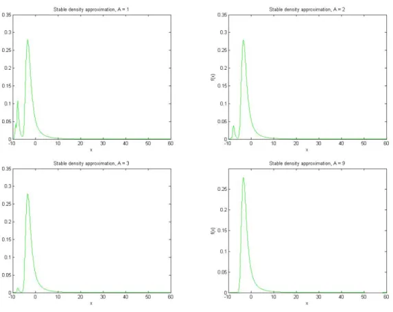
Example 2.2.2. Let f be the density of a stable distribution with the skewness parameter β = 1 and the location parameterη = 0. The log Laplace transformation is given by
logµ∗(t) =
− cαtα cos(πα
2 )
, if α 6= 1,
2ct
π logt, if α = 1,
(2.2.7)
where t∈C,<(t)>0 and c is the scale parameter. It is known (e.g. Zolotarev [29], Samorodnitsky and Taqqu [25]) that the stable density is concentrated on the whole real line. But whereas its right tail is heavy-tailed, the left tail has an exponential decay. To numerically calculate the densityf by using the method of Section 2.1, we shift f to the right by a margin of S >0 by considering the density f(x+S). After numerically calculating the density f(x+S), we shift it to the left by a margin of S to get the density f.
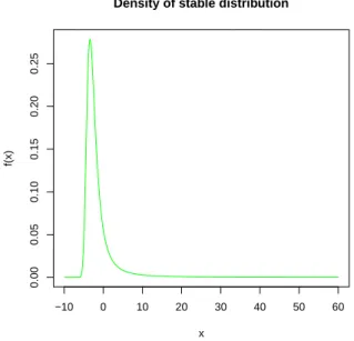
Figure 2.2 presents the plots of the density approximation on the interval −9.9 to 60 for the choices of A= 1, 2, 3 and 9. We have used the value ofS = 10 for the shift of the density. Figure 2.3 presents the plot of the actual density of the stable distribution (obtained using the R functiondstable in the packagestabledist) showing an agreement with the numerical calculation in Figure 2.2, when A = 9. Such larger values of A are also recommended by Abate and Whitt [1].
2.3 Semi-stable densities
Figure 2.2: Stable density with α= 1.2, c= 1, β= 1.
distribution appearing in the limit of their domain of attraction. This will be carried out by comparing the histograms of the partial sums and the corresponding densities of the semi-stable distributions. The findings of the section will serve as a guide in the applications of semi-stable laws to sampling (Chapter 4).
We thus begin with a distribution in the domain of attraction of a semi-stable law according to the theorems in Section 2.1 and characterize the characteristic function of the limiting semi-stable distribution. We shall follow the notation consistent with the sampling framework briefly discussed in Section 1.1 and further developed in Chapters 3 and 4.
Example 2.3.1. Let X, X1, X2, . . . be a sequence of i.i.d. random variables defined
as
−10 0 10 20 30 40 50 60
0.00
0.05
0.10
0.15
0.20
0.25
Density of stable distribution
x
f(x)
Figure 2.3: Plot of actual stable density with α= 1.2, c= 1, β = 1.
where β >0 and Wq follows a geometric distribution with parameter s∈(0,1), that
is, its p.m.f. is
fWq(x) =sx−1(1−s), x= 1,2, . . . . (2.3.1)
We shall apply Theorem 2.1.1 to show that, depending on the choices of s and β, the distribution F of X is in the domain of attraction of a semi-stable distribution. We shall also derive the sequences {Akn},{Bkn}and {kn} for the convergence of the
corresponding partial sums (2.1.4).
First, observe that
1−F(x) = P(X > x) = P(eβWq > x) =P(Wq>
1
β logx) = 1 ss
d1
βlogxe+
= 1 sx
−β1log1s
sd1βlogxe+− 1
βlogx, (2.3.2)
wheredxe
suggests α= 1 β log
1
s. Now, consider
MR(x) = e
−log(1s)(d1
βlogxe+− 1
βlogx),
which is a right-continuous function with a multiplicative periodeβ =c1α with c= 1 s.
Taking Akn =eβ(n−1), we have
δ(x) = x
eβ(n−1), if e β(n−1)
≤x < eβn.
Then, when α = β1 log1s < 2, the right-hand side of (2.3.2) is exactly of the form (2.1.8) with hR(x) ≡ 0 and l∗(x) = 1s. Hence, F is in the domain of attraction of a
semi-stable law.
We derive the form of kn by first defining the sequence ˜An as described following
Theorem 2.1.1. According to (2.1.12), we need to have limn→∞nsA˜−nα = 1. So, we
define
˜ An = (
n s)
1
α.
By (2.1.14), kn are then defined as the natural numbers satisfying
(kn s )
1
α ≤eβ(n−1) <(kn+1
s ) 1
α.
Substituting α= β1 log1s above, we get
kn≤(
1 s)
n−2 < k n+1,
The centering constants {Bkn}can be obtained from (2.1.15) and (2.1.16),
involv-ing the quantile function Q. We shall derive the asymptotic behavior of the quantity
Bkn Akn =
kn Akn
R1−
1
kn
1
kn
Q(t)dt for two different cases 0 < α <1 and 1 < α < 2. The func-tion Q(t) is defined as the inverse of the distribution function F(x) = P(eβWq ≤x).
The function F(x) has jumps at points x = eβn of sizes (1−s)sn−1, n ≥ 1. This
means that the inverse function Q(t) has jumps at points t= 1−sm, m≥1, of sizes eβ(m+1)−eβm=eβm(eβ−1). Moreover,Q(t) = eβmwhen 1−sm−1 ≤t <1−sm, m≥1. Also note that eβs>1 when 0< α <1 andeβs <1 when 1 < α <2.
Assume for simplicity that 1s is an integer so that kn= (1s)n−2. Then,
kn
Akn
Z 1−kn1
1
kn
Q(t)dt= kn Akn
Z 1−kn1
0
Q(t)dt− kn Akn
Z kn1
0
Q(t)dt.
Now,
kn
Akn
Z kn1
0
Q(t)dt∼ kn Akn
1−s kn
= 1−s Akn →
0.
Moreover,
kn
Akn
Z 1−kn1
0
Q(t)dt = kn Akn
n−2
X
m=1
eβm(sm−1−sm)
= e−β( 1 eβs)
n−2 n−2
X
m=1
eβ(1−s)(eβs)m−1
= (1−s)
n−2
X
m=1
(eβs)m+1−n
= (1−s)e−βs−11−(e
βs)1−n
1−e−βs−1 →
1−s eβs−1.
Hence, when 0 < α < 1, Akn
kn
R1−kn1
1
kn
Q(t)dt → ζ = e1β−s−s1. When 1 < α < 2, it can
be shown that knE(X)−Bkn
R1
0 Q(t)dt, observe that
knEX−Bkn
Akn
= kn Akn
Z kn1
0
Q(t)dt+ kn Akn
Z 1
1− 1
kn
Q(t)dt∼ kn Akn
Z 1
1− 1
kn
Q(t)dt
= kn Akn
Z 1
1−sn−2
Q(t)dt= kn Akn
∞ X
m=n−1
eβm(sm−1 −sm)→ 1−s 1−eβs.
Hence, for 1< α <2, knE(X)−Bkn
Akn → −ζ =
1−s 1−eβs.
For this example, the log of the characteristic function of the semi-stable distri-bution can be derived as follows. Note that the L´evy measure is characterized by the (distribution) function
R(x) =−e−log(1s)(d
1
βlogxe+− 1
βlogx)x−
1
βlog
1
s =−e−log(
1
s)(d
1
βlogxe+) =−sd 1
βlogxe+.
The function R is right-continuous with jumps at ekβ taking values −sk+1, where
k ∈ Z. Hence, by combining (2.1.2), (2.1.3) and (2.1.17), (2.1.18), (2.1.19), we get the log characteristic function as
logµ(t) =b −i(η−ζ)t+
∞ X
k=−∞
(eitekβ −1− e
kβ
1 +e2kβ)(1−s)s k , (2.3.3) where η= 0 X k=−∞ e3kβ
1 +e2kβs k
(1−s)−
∞ X
k=0
ekβ
1 +e2kβs k
(1−s). (2.3.4)
for some 0< δ <2,
lim inf
r→0
R
[0,r]x
2dR(x)
r2−δ >0. (2.3.5)
In the example considered here, the relation (2.3.5) holds with δ=α since
lim
m→−∞ R
[0,eβm]x2dR(x)
eβm(2−α) = mlim→−∞
Pm
k=−∞e2kβ(1−s)sk
eβm(2−α)
= lim
m→−∞
(1−s)smeβmα
1−e−2βs−1 →
1−s 1−e−2βs−1
since seβα = 1.
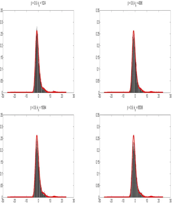
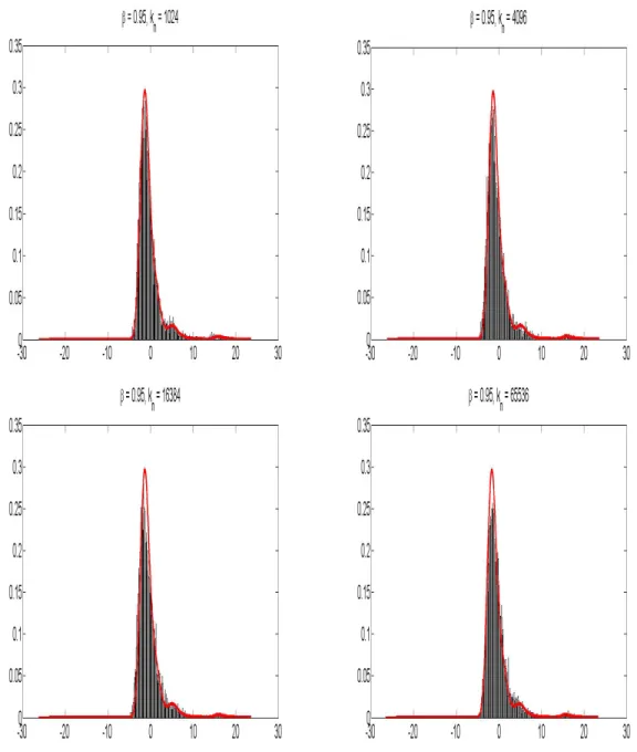
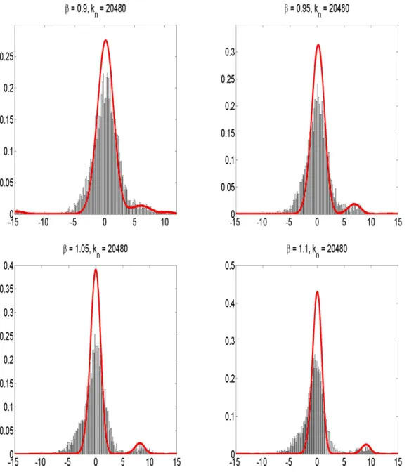
Using the characteristic function in (2.3.3) and the Abate and Whitt [1] method, we are going to compute numerically the density of the limiting semi-stable density for this example and also compare it to the histograms of the partial sums Sn. We
fix s = 0.25 but vary the value of β such that α = β1log 1s < 2. Figures 2.4–2.8 are associated with β = 0.85,0.9,0.95,1.05 and 1.1, respectively. In each of these figures, four plots are presented corresponding to n = 7,8,9,10 so that kn takes
values 1024,4096,16384 and 65536. For each of these cases, we numerically calculate the density of the limiting semi-stable distribution (centered at 0; in red solid curve) and also plot the histogram of the empirical distribution of the partial sum Sn.
From the figures, the agreement between the numerically calculated density and the empirical histogram is very good for smaller values of β = 0.85,0.9 and 0.95. As β increases and especially becomes larger than 1, the numerically calculated density deviates from the the empirical histogram. Note, however, that the agreement is quite good in the two tails in all the cases considered.
Finally, note that the approximation is expected to be worse as β increases. In-deed, asβ becomes larger, the random variable eβX takes values separated by wider
values of n and hence kn to converge to the limiting semi-stable distribution.
CHAPTER 3: SEMI-STABLE DOMAINS OF ATTRACTION
This chapter contains our main results on the convergence to semi-stable distri-butions. In Section 3.1, we give a general practical result for a distribution function to be in the domain of attraction of semi-stable distribution. We explicitly derive the normalizing and centering constants, and the form of subsequence along which the convergence of partial sums to the semi-stable distribution takes place. We also consider the behavior of partial sums along all natural numbers instead of a suitable subsequence. In Section 3.2, we illustrate the results of Section 3.1 with concrete example. We also numerically calculate the density of the limiting semi-stable distri-bution for the example and assess how well it approximates the empirical histograms of partial sums in finite samples.
3.1 General results
The next theorem is the main result of this dissertation. We use the following notation throughout this dissertation:
dxe= the smallest integer larger than or equal to x, dxe
+ = the smallest integer strictly larger than x.
For example, d2.47e = d2.47e
+ = 3 but d3e = 3 and d3e+ = 4. The function dxe+ is the right-continuous version of the function dxe. Also note that dxe
Theorem 3.1.1. LetWq be an integer-valued random variable taking values in0,1,2, . . .
such that, for all x >0,
P
Wq
2 ≥x, Wq is even
=
∞ X
n=dxe
P
Wq
2 =n
=h1(dxe)e−νdxe, (3.1.1)
P
Wq−1
2 ≥x, Wq is odd
=
∞ X
n=dxe
P
Wq−1
2 =n
=h2(dxe)e−νdxe, (3.1.2)
where ν >0 and the functions h1 and h2 satisfy
h2(x)
h1(x) →
c1, as x→ ∞, (3.1.3)
for some fixed c1 ≥0, and
h1(ax)
h1(x) →
1 as x→ ∞, a→1. (3.1.4)
Let also
X =L(eWq)eβWq(−1)Wq, (3.1.5)
where β > 0 and L is a slowly varying function at ∞ such that L(en) is ultimately
monotonically increasing. Suppose that
α:= ν
2β <2. (3.1.6)
Then, X is in the domain of attraction of a semi-stable distribution in the following sense. If X, X1, X2, . . . are i.i.d. random variables, then as n→ ∞, the partial sums
1 Akn
kn
X
j=1
Xj−Bkn
converge to a semi-stable distribution with
kn=
e(n−1)ν
h1(n−1)
, Akn =L(e2n−2)e2β(n−1) (3.1.8)
and Bkn given by (2.1.15). The limiting semi-stable distribution is non-Gaussian,
has location parameter given in (2.1.17) and is characterized by
α = ν
2β, (3.1.9)
ML(−x) =c1e
−ν([12+21βlogx]−1
2βlogx), M
R(x) = e
−ν(d1
2βlogxe+− 1
2βlogx), x >0.
(3.1.10)
Before giving a proof of Theorem 3.1.1, let us explain its novelty, especially when compared to the available Theorems 2.1.1 and 2.1.2 on the domains of attraction of semi-stable distributions. Note that if L appearing in (3.1.5) is constant, then the convergence of the partial sums (3.1.7) to a semi-stable distribution can easily be deduced from Theorem 2.1.1. Taking L(x) = 1 without loss of generality,
¯
F(x) := 1−F(x) = P(eβWq(−1)Wq > x) = P(Wq
2 > 1
2β logx, Wq
2 is an integer) = h1(d
1
2β logxe+)e
−νd1 2βlogxe+
= x−2νβh 1(d
1
2βlogxe+)e
−ν(d1
2βlogxe+− 1 2βlogx)
= x2νβl∗(x)M
R(δ(x)), (3.1.11)
e2βn if e2βn ≤x < e2β(n+1). It can be shown that l∗ is a slowly varying function, and
hence that (3.1.11) is of the form (2.1.8). Similarly, it can be shown that the left tail of the distribution function of the random variable eβWq(−1)Wq can be expressed as
(2.1.7).
Similarly, when the functions h1 and h2 appearing in (3.1.1) and (3.1.2) are
con-stant, the convergence of the partial sums (3.1.7) to a semi-stable distribution can be deduced easily from Theorem 2.1.2. In this case, taking h1(x) ≡ h2(x) ≡ 1 for
simplicity, consider first the quantile functionQcorresponding to the right tail of F. We have
Q(1−s) = inf
y {F(y)≥1−s}
= inf
y {P(L(e
Wq)eβWq(
−1)Wq ≤y, Wq is an even number)≥1−s}
= inf
y {P(L(e
2Z)e2βZ ≤y)≥1−s}, (3.1.12)
where Z = Wq2 and Z is an integer. Note from (3.1.1) that P(Z ≥ x) = e−νdxe and hence P(Z > x) = e−νdxe+. Then, P(Z ≤x) = 1−P(Z > x) = 1−e−νdxe+ and to solve (3.1.12), consider the equation
x= inf
t {1−e
−νdte
+ ≥1−s}. (3.1.13)
The inequality in (3.1.13) becomes
dte + ≥
1 ν log
1
s, (3.1.14)
leading to the solution
x=d1 νlog
1
Turning back to (3.1.12), we havey=L(e2x)e2βx =L(e−2ed1
νlog
1
se)e−2βed
1
νlog
1
sewhich
has the form (2.1.21). One can show similarly that the left tail of the quantile function Q is also of the form (2.1.20).
If one of the functions h1 or h2 is non-constant and L is also non-constant, then
proving the convergence of the partial sums (3.1.7) to a semi-stable distribution is not so trivial. The main purpose of Theorem 3.1.1 is to show how this can be done using Theorem 2.1.1. We also characterize the normalizing constants Akn, centering
constants Bkn and the subsequence kn along which the sequence of partial sums
converges. We also present the explicit form of the log characteristic function for the limiting semi-stable distribution.
Proof of Theorem 3.1.1. The result will be proved by verifying the sufficient conditions (2.1.7)–(2.1.8) of Theorem 2.1.1. We break the proof into two cases dealing with (2.1.7) and (2.1.8) separately. The final part of the proof shows that the sequence kn can be chosen as in (3.1.8)
Case 1 (showing (2.1.8)): Fix x > 0 large enough. In view of (3.1.5), we are interested in
¯
F(x) := 1−F(x) = P
L eWqeβWq(−1)Wq > x
. (3.1.16)
LetZ2 = Wq2 . Note that (3.1.16) can be written as
¯
F(x) = P
L(e2Z2)e2βZ2 > x, Z
2 is integer
= P
L(e2Z2)e2βZ2 > x
= P
Z2+
1
2β logL e
2Z2 > 1 2β logx
where, in view of (3.1.1),
P(Z2 ≥x) =h1(dxe)e−νdxe. (3.1.18)
We next want to write ¯F(x) in (3.1.17) as
¯
F(x) =P
Z2 ≥g
1 2β logx
(3.1.19)
for some function g.
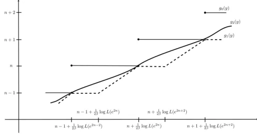
There are many choices for g in (3.1.19). One natural choice is to take
g0(y) = n, if (n−1) +
1
2β logL e
2n−2
≤y < n+ 1
2β logL e
2n
. (3.1.20)
The function g0, however, is not suitable for our purpose. We will use a function g1
defined, for integer n ≥2, as
g1(y) =
n−1, if n−1 + 2β1 logL(e2n−2)≤y < n−1 + 2β1 logL(e2n), y− 2β1 logL(e2n), if n−1 + 2β1 logL(e2n)≤y < n+ 2β1 logL(e2n).
(3.1.21) We will also use the function
g2(y) =f−1(y) = inf{z:f(z)≥y} (3.1.22)
defined as an inverse of the function
f(z) = z+ 1
2βlogL e
2z
n
n−1 n+ 1 n+ 2
n+ 1 2βlogL(e2n) n−1 + 1
2βlogL(e2n−2) n+ 1 +
1
2βlogL(e2n+2) n−1 + 1
2βlogL(e2n) n+21βlogL(e2n+2)
g0(y)
g2(y)
g1(y)
Figure 3.1: Plot of g0(y), g1(y) andg2(y).
Note that
dg0(y)e=dg1(y)e+ =dg2(y)e+ =dg(y)e, (3.1.24)
where g is any function satisfying (3.1.19). The functions g0, g1 and g2 are plotted
in Figure 3.1.
We shall use another function ˜g1 which modifiesg1in the following way: forn≥2,
˜
g1(y) =y−
1
2βlogL(e
2n−2), if n
−1 + 1
2βlogL(e
2n−2)
≤y < n+ 1
2β logL(e
2n).
(3.1.25)
One relationship between the functions g1 and ˜g1 can be found in Lemma A.1.1 in
Appendix A.1, and will be used in the proof below. Note that ˜g1(y) can be expressed
as
˜
where, forn ≥2,
˜
g∗1(y) = 1
2βlogL e
2n−2
, if n−1 + 1
2β logL(e
2n−2)
≤y < n+ 1
2βlogL(e
2n).
(3.1.27) See Lemma A.1.2 in Appendix A.1 for a property of ˜g∗1 which will be used in the proof below.
We need few properties of the function g2. Since g2 is the inverse of the function
f, we have eg2(logx) as the inverse of ef(logx). Indeed,
eg2(logef(logx)) =eg2(f(logx)) =elogx =x.
Note now from (3.1.23) that
ef(logx) =elogx+21βlogL(x
2)
=x L(x2) 1 2β .
Since (L(x2))21β is a slowly varying function, ef(logx) is a regularly varying function.
So, by Theorem 1.5.13 of Bingham, Goldie and Teugels [3],
eg2(logx)=xl(x),
where l(x) is a slowly varying function. Hence,
g2(log x) = logx+ log l(x) = logx+g2∗(log x),
where
or replacing log x byy,
g2(y) = y+g∗2(y). (3.1.28)
Note also that for any A >0, we have
g2∗(log Ax)−g∗2(log x) = log l(Ax)−log l(x) = log l(Ax)
l(x) →0, asx→ ∞. (3.1.29)
Continuing with (3.1.19) now, note that, by using (3.1.18) and (3.1.24),
¯
F(x) = P
Z2 ≥g
1 2β logx
= h1
dg( 1
2β logx)e
e−νdg(21βlogx)e
= h1
dg2(
1
2β logx)e+
e−νdg1(21βlogx)e+. (3.1.30)
By using (3.1.26), note further that
¯
F(x) = h1
dg2(
1
2β logx)e+
e−ν˜g1(21βlogx) ·
e−ν(g1(21βlogx)−˜g1(21βlogx))e−ν(dg1(21βlogx)e+−g1(21βlogx))
= h1
dg2(
1
2β logx)e+
e−ν(21βlogx−g˜
∗
1(21βlogx))·
e−ν(g1(21βlogx)−˜g1(21βlogx))e−ν(dg1(21βlogx)e+−g1(21βlogx))
where α= ν
2β as given in (3.1.81),
l1∗(x) = h1
dg2(
1
2β logx)e+
eνg˜1∗( 1
2βlogx)e−ν(g1(
1
2βlogx)−˜g1(
1
2βlogx)), (3.1.32)
MR(δ(x)) =e
−ν(d˜g1(21βlogx)e+−g˜1(21βlogx))
(3.1.33)
and
hR(x) = e
−ν(dg1(21βlogx)e+−g1(21βlogx))
−e−ν(d˜g1(21βlogx)e+−g˜1(21βlogx))
. (3.1.34)
We next show that the functions l1∗, MR and hR satisfy the conditions of Theorem
2.1.1 with suitable choices of δ(x) and Akn.
By Lemma A.1.3 in Appendix A.1, l1∗(x) is a right-continuous slowly varying function and hence it satisfies the conditions of Theorem 2.1.1. For the function MR(δ(x)), note from (3.1.33) that
MR(δ(x)) = e
−ν
2β˜g1(1
2βlogx)
2β
+
−2β˜g1(
1 2βlogx)
2β
= MR
e2β˜g1(21βlogx)
(3.1.35)
with
MR(x) =e
−ν(dlog2βxe
+− logx
2β ). (3.1.36)
The functionMR(x) is periodic with multiplicative periode2β, and is right-continuous
as required in Theorem 2.1.1. Since the periode2β is also c1α, this yields
To choose δ(x), note from (3.1.35) that
MR(δ(x)) =MR
e2β˜g1(21βlogx)−2β(n−1)
,
for any n≥1, since MR has multiplicative period e2β. We can set
δ(x) =e2βg˜1(21βlogx)−2β(n−1)
, if e2β(n−1)L(e2n−2)≤x < e2nβL(e2n). (3.1.38)
From (3.1.25), we have
δ(x) = e2β(21βlogx−
1 2βlogL(e
2n−2))−2β(n−1)
= x
e2β(n−1)L(e2n−2), if e
2β(n−1)L(e2n−2)
≤x < e2nβL(e2n). (3.1.39)
Thus,δ(x) has the required form (2.1.10)–(2.1.11) with
Akn =e2β(n−1)L(e2n−2) (3.1.40)
and
a(x) =e2β(n−1)L(e2n−2) = Akn, if Akn ≤x < Akn+1. (3.1.41)
Note also from (3.1.39) that
1≤δ(x)< e
2βnL(e2n)
e2β(n−1)L(e2n−2) =e
2β L(e2n)
L(e−2e2n) →e 2β
=cα1,
so that δ(x)∈[1, cα1 +] for large enough x when >0 is fixed.
continuity point x0 of MR(x). The discontinuity points of MR are
x=e2kβ, k ∈Z. (3.1.42)
To show hR(Aknx0) → 0, note that, by Lemma A.1.1, it is enough to prove that
˜
hR(Aknx0)6= 0 for finitely many values of n, where
˜
hR(x) =e
−νdg1(21βlogx)e+
−e−νd˜g1(21βlogx)e+ .
This holds only if for some integer m≥2,
m+ logL(e2m−2)≤ 1
2βlogAknx0 < m+ logL(e
2m). (3.1.43)
By Lemma A.1.4, (3.1.43) holds for infinitely many values of n only if x0 = e2rβ,
r∈Z, which is a discontinuity point of MR(x) in (3.1.42). Hence, hR(Aknx0)→0 as
n→ ∞ for every continuity point x0 of MR(x).
Case 2 (showing (2.1.7)): In view of (3.1.5), we are now interested in
F (−x) = P
L eWqeβWq(−1)Wq <−x
LetZ2 = Wq2 as in Case 1. Note that (3.1.44) can be written as
F (−x) = P
L e2Z2e2βZ2 > x, Z
2−
1
2 is integer
= P
L ee2(Z2−12)eβe2β(Z2−12) > x, Z
2−
1
2 is integer
= P
L(ee2Z1)eβe2βZ1 > x
= P
Z1+
1 2+
1
2β logL(e
2Z1+1)> 1 2βlog x
, (3.1.45)
where, in view of (3.1.2),
P(Z1 ≥x) =h2(dxe)e−νdxe. (3.1.46)
Writing (3.1.45) as
F (−x) =P
Z1+
1
2βlogL(e
2Z1+1)> 1
2βlog x− 1 2
,
the right-hand side has the form (3.1.16) where L(e2Z2) is replaced by L(ee2Z1) and
1
2β logx is replaced by 1
2βlogx− 1
2. Thus, as in (3.1.19)–(3.1.20), one can write
F (−x) =P
Z1 ≥g(˜
1
2β logx− 1 2) , (3.1.47) where ˜
g(y) =n, if n−1 + 1
2β logL(ee
2n−2)
≤y < n+ 1
2βlogL(ee
The expression (3.1.47) can also be written as
F (−x) =P
Z1 ≥g˜0(
1
2β logx)
, (3.1.49)
where ˜g0(y) = ˜g(y− 12) or, forn ≥2,
˜
g0(y) =n, if n−
1 2 +
1
2βlogL(e
2n−1
)≤y < n+ 1 2+
1
2β logL(e
2n+1
). (3.1.50)
We want to work with the intervals [n−1 + 2β1 logL(e2n−2), n+ 1
2β logL(e 2n))
appearing in Case 1, and use the results of that case. Note that, on the interval [n−1 + 2β1 logL(e2n−2), n+ 1
2βlogL(e
2n)), the function ˜g
0 takes values as
˜ g0(y) =
n−1, if n−1 + 2β1 logL(e2n−2)≤y < n− 1 2 +
1
2βlogL(e 2n−1),
n, if n− 12 + 2β1 logL(e2n−1)≤y < n+ 1
2β logL(e 2n).
(3.1.51) Defining
I0(y) =
−1, if n−1 + 2β1 logL(e2n−2)≤y < n− 12 + 2β1 logL(e2n−1), 0, if n−12 + 2β1 logL(e2n−1)≤y < n+ 2β1 logL(e2n),
(3.1.52)
and combing (3.1.20), (3.1.51) and (3.1.52), we have
˜
Continuing with (3.1.49), note further that, by using (3.1.46) and (3.1.53),
F(−x) = h2
˜ g0(
1
2βlogx)
e−ν˜g0(21βlogx)
= e−νI0(21βlogx)h
2
g0(
1
2βlog x) +I0( 1
2βlog x)
e−νg0(21βlogx).(3.1.54)
We want to write F(−x) as in (2.1.7) of Theorem 2.1.1 (where by Lemma A.1.5, we can take a slowly varying function l2∗ which is asymptotically equivalent to l1∗). We need the notation for the intervals appearing in (3.1.51)–(3.1.52), namely, for n≥1,
Dn = [n−1 +
1
2βlog L(e
2n−2), n
− 1 2+
1
2βlog L(e
2n−1)),
En = [n−
1 2+
1
2βlog L(e
2n−1), n+ 1
2βlog L(e
2n)).
We also need a similar notation without the slowly varying function L, that is, for n≥1,
D0n= [n−1, n− 1
2), E 0
n = [n−
1 2, n).
Set also
D=
∞ [
n=1
Dn, E =
∞ [
n=1
En, D
0 =
∞ [
n=1
Dn0, E0 =
∞ [
n=1
En0. (3.1.55)
As in (3.1.31), we can now write (3.1.54) as
F (−x) = x−αh2(g0(
1
2βlog x) +I0( 1
2βlog x))
c1h1(g0(2β1 log x))
l1∗(x)c1e−νI0(
1
2βlogx)e−ν(dg1(
1
where α= ν
2β and l
∗
1(x) is given in (3.1.32). This can also be written as
F(−x) = x−αl2∗(x)(ML(−δ(x)) +hL(x)),
where
l∗2(x) = h2(g0(
1
2βlog x) +I0( 1
2βlog x))
c1h1(g0(2β1 log x))
l1∗(x), (3.1.56)
ML(−δ(x)) = c1e
−ν([12+˜g1(21βlogx)]−˜g1(21βlogx)), (3.1.57)
hL(x) =c1e
−νI0(21βlogx)e−ν(dg1(21βlogx)e+−g1(21βlogx)) −c1e
−ν([12+˜g1(21βlogx)]−g˜1(21βlogx)).
(3.1.58)
By using (3.1.3)–(3.1.4), we have
h2(g0(2β1 log x) +I0(2β1 log x))
c1h1(g0(2β1 log x)) →
1, asx→ ∞.
Hence, l∗2(x)
l∗1(x) →1, asx→ ∞, that is,l
∗
2(x) andl∗1(x) are two asymptotically equivalent
functions. By the definition of I0 and using Lemma A.1.3, l∗2(x) is right-continuous
and slowly varying.
The functionδ(x) appearing in (3.1.57) is the same as in (3.1.38)–(3.1.39) of Case 1, while the functionML(−x) is defined as
ML(−x) = c1e
−ν([12+21βlogx]−1
2βlogx), x >0. (3.1.59)
discontinuity points of ML(−x) are
x=eβ(2k+1), k ∈Z. (3.1.60)
To conclude the proof of Case 2, we need to show that hL(Aknx0)→0 as n→ ∞
for every continuity point x0 of ML(−x), that is, x0 different from (3.1.60). For this,
we rewritehL(x) as follows. Observe that
e−νI0(y) =eν1
D(y) + 1E(y)
and
(eν1D0(y) + 1
E0(y))e
−ν(dye
+−y) =e−ν([ 1 2+y]−y),
where after taking the logs, using dye
+ = [y] + 1 and simplification, the last identity is equivalent to [y]1D0(y) + ([y] + 1)1
E0(y) = [ 1
2+y] and can be seen easily by drawing
a picture. By using these identities and (3.1.58), we can write
c−11hL(x) = (eν1D(
1
2βlogx) + 1E( 1
2β logx))e
−ν(dg1(21βlogx)e+−g1(21βlogx))
−e−ν([12+˜g1( 1
2βlogx)]−˜g1(
1 2βlogx))
= h1,L(x)e
−ν(dg1(21βlogx)e+−g1(21βlogx))
+h2,L(x),
where
h1,L(x) =eν1D(
1
2βlog x) + 1E( 1
2βlog x)−e
ν1 D0(g1(
1
2βlog x))−1E0(g1( 1
2βlog x)),
h2,L(x) =e−ν([
1 2+g1(
1
2βlogx)]−g1(
1
2βlogx))−e−ν([
1 2+˜g1(
1
2βlogx)]−g˜1(
It is therefore enough to show thath1,L(Aknx0)→0 andh2,L(Aknx0)→0, as n→ ∞.
From (3.1.21), (3.1.25) and (3.1.55), h1,L(Aknx0)6= 0 if, for some integer m≥1,
m− 1
2+ logL(e
2m−1)
≤ 2β1 logAknx0 < m−
1
2+ logL(e
2m). (3.1.61)
(To see this, partition [m−1 + 2β1 logL(e2m−2), m+ 2β1 logL(e2m)) into four subin-tervals [m−1 + 2β1 logL(e2m−2), m−1 + 2β1 logL(e2m)), [m−1 + 2β1 logL(e2m), m−
1 2 +
1
2β logL(e
2m−1)), [m − 1 2 +
1
2β logL(e
2m−1), m − 1 2 +
1
2β logL(e
2m)), [m − 1 2 + 1
2β logL(e
2m), m+ 1
2βlogL(e
2m)) and check that the function is nonzero only on the
third subinterval as given in (3.1.61).) By Lemma A.1.4, (3.1.61) holds for infinitely many values of n only if x0 = eβ(2r+1) which is a discontinuity point of ML(−x) in
(3.1.60). To showh2,L(Aknx0)→0, note that, by Lemma A.1.1, it is enough to prove
that ˜h2,L(Aknx0)6= 0 for finitely many values of n, where
˜
h2,L(x) =e−ν[
1 2+g1(
1
2βlogx)]−e−ν[
1 2+˜g1(
1 2βlogx)].
By using (3.1.21) and (3.1.25), the relation ˜h2,L(Aknx0) = 0 holds only if, for some
integer m≥1,
m− 1
2+ logL(e
2m−2)≤ 1
2β logAknx0 < m− 1
2+ logL(e
2m). (3.1.62)
(To see this, draw a plot of g1(y) and ˜g1(y) for y in [m−1 + 2β1 logL(e2m−2), m− 1
2logL(e
2m)), and note that ˜g
1(y) = m − 12 at y = m − 12 + 2β1 logL(e2m−2) and
g1(y) =m− 12 + 2β1 logL(e2m).) By Lemma A.1.4, (3.1.62) holds for infinitely many
values ofn only if x0 =eβ(2r+1) which is a discontinuity point ofML(−x) in (3.1.60).
Deriving subsequence kn: We conclude the proof of the theorem by showing that
kn is given by (3.1.8). In view of the discussion following Theorem 2.1.1, we want to
choose a sequence ˜An satisfying (2.1.12)–(2.1.13) such that kn given by (3.1.8) now
satisfies (2.1.14). We define such sequence ˜An as
log ˜An = 2β(m−1) + logL(e2m−2)
+ (log n−log km)(2β+ log L(e
2m)−log L(e2m−2))
log km+1−log km
if km ≤n < km+1, m≥1. (3.1.63)
The sequence ˜An satisfies (2.1.13). For example, if km ≤n < km+1−1, the last limit
in (2.1.13) follows from
log ˜An+1−log ˜An=
(log n−log (n+ 1))(2β+ log L(e2m)−log L(e2m−2))
log km+1−log km →
0.
If n=km+1−1, the limit follows from
log ˜An+1−log ˜An= 2β+ logL(e2m)−logL(e2m−2)
−(log (km+1−1)−log km)(2β+ log L(e
2m)−log L(e2m−2))
log km+1−log km →
0
since logL(e2m)−logL(e2m−2)→0, and
log (km+1−1)−log km
log km+1−log km →
1.
is as defined in (3.1.32). When km ≤n < km+1, observe that
lognA˜−nαl1∗( ˜An) = log
nl∗1( ˜An)
˜ Aν/2βn
= log nl
∗
1( ˜An)
e(m−1)νL(e2m−2)ν/2β +
ν+ 2βν log L(e2m)− ν
2βlog L(e 2m−2)
log km+1−log km
log km n
!
∼ logn+ log l
∗
1( ˜An)
h1(m−1)L(e2m−2)ν/2β −
logkm
+ν+
ν
2βlog L(e
2m)− ν
2βlog L(e 2m−2)
log km+1−log km
log km n
!
. (3.1.64)
Now observe that as n → ∞, we have m → ∞, and thus kmn is bounded and
ν+ 2βν log L(e2m)−2βν log L(e2m−2) log km+1−log km →
1.
Thus, (3.1.64) is asymptotically equivalent to
log l
∗
1( ˜An)
h1(m−1)L(e2m−2)ν/2β
. (3.1.65)
By the relation (A.1.4) in Appendix A.1, l1∗( ˜An)∼h1(g2(2β1 log ˜An))eν˜g
∗ 1(
1
2βlog ˜An) and
hence (3.1.64) is also asymptotically equivalent to
logh1(g2(
1
2βlog ˜An))e
νg˜1∗(21βlog ˜An)
h1(m−1)L(e2m−2)ν/2β
. (3.1.66)
Since km ≤n < km+1, we have
2β(m−1) + logL(e2m−2)≤log ˜An<2βm+ logL(e2m)
and, by (3.1.27), e
νg˜∗1 (1 2βlog ˜An)
L(e2m−2)ν/2β = 1. Hence, (3.1.66) simplifies to log
h1(m−1+κ)
κ < 1. But as n → ∞, we have m → ∞ and thus h1(m−1+κ)
h1(m−1) → 1 by using (3.1.4). This proves that lognA˜−α
n l
∗
1( ˜An)→0 and thus nA˜−nαl
∗
1( ˜An)→1, as n → ∞.
Finally, we show that kn defined in (3.1.8) satisfies (2.1.14). Define an = Akn =
e2β(n−1)L(e2n−2). Hence,
logan= logAkn = 2β(n−1) + logL(e2n−2).
Now observe that ˜Akn =an and thus (2.1.14) is satisfied.
The partial sums (3.1.7) involve centering constants Bkn defined in (2.1.15). As
in the stable case, one can expect to replace Bkn by knEX when 1 < α <2, and to
show the convergence of (3.1.7) without Bkn when 0< α <1. The next result shows
that this is indeed the case.
Proposition 3.1.1. Suppose that the assumptions of Theorem 3.1.1 hold. Let
ζ = − 1−e
−ν
1−e2β−ν −e β(2d1
νlogc1e−1)(c1e−ν(d
1
νlogc1e−1)−1)
+ c1
(1−e−ν)eν−β
1−e2β−ν e
(2β−ν)d1
νlogc1e. (3.1.67)
If 0< α <1, then
Bkn
Akn →
ζ, 1
Akn kn
X
j=1
Xj d
→Y +ζ
and if 1< α <2, then
knEX−Bkn
Akn → −
ζ, 1
Akn
kn
X
j=1
Xj −knEX
d
→Y +ζ,