DOI:10.1051/0004-6361/201423877 c
ESO 2014
Astrophysics
&
L
etter to the
E
ditor
Rapidly increasing collimation and magnetic field changes
of a protostellar H
2
O maser outflow
G. Surcis
1, W. H. T. Vlemmings
2, H. J. van Langevelde
1,3, C. Goddi
1, J. M. Torrelles
4, J. Cantó
5, S. Curiel
5,
S.-W. Kim
6, and J.-S. Kim
71 Joint Institute for VLBI in Europe, Postbus 2, 79990 AA Dwingeloo, The Netherlands
e-mail:[email protected]
2 Chalmers University of Technology, Onsala Space Observatory, 439 92 Onsala, Sweden 3 Sterrewacht Leiden, Leiden University, Postbus 9513, 2300 RA Leiden, The Netherlands
4 Institut de Ciències de l’Espai (CSIC)-Institut de Ciències del Cosmos (UB)/IEEC, 08028 Barcelona, Spain 5 Instituto de Astronomía (UNAM), Apdo Postal 70-264, Cd. Universitaria, 04510-Mexico D.F., Mexico
6 Korea Astronomy and Space Science Institute, 776 Daedeokdaero, Yuseong, 305-348 Daejeon, Republic of Korea 7 National Astronomical Observatory of Japan, 2-21-1 Osawa, Mitaka, 181-8588 Tokyo, Japan
Received 25 March 2014/Accepted 30 April 2014
ABSTRACT
Context.W75N(B) is a massive star-forming region that contains three radio continuum sources (VLA 1, VLA 2, and VLA 3), which are thought to be three massive young stellar objects at three different evolutionary stages. VLA 1 is the most evolved and VLA 2 the least evolved source. The 22 GHz H2O masers associated with VLA 1 and VLA 2 have been mapped at several epochs over eight
years. While the H2O masers in VLA 1 show a persistent linear distribution along a radio jet, those in VLA 2 are distributed around
an expanding shell. Furthermore, H2O maser polarimetric measurements revealed magnetic fields aligned with the two structures.
Aims.Using new polarimetric observations of H2O masers, we aim to confirm the elliptical expansion of the shell-like structure
around VLA 2 and, at the same time, to determine if the magnetic fields around the two sources have changed.
Methods. The NRAO Very Long Baseline Array was used to measure the linear polarization and the Zeeman-splitting of the
22 GHz H2O masers towards the massive star-forming region W75N(B).
Results.The H2O maser distribution around VLA 1 is unchanged from that previously observed. We made an elliptical fit of
the H2O masers around VLA 2. We find that the shell-like structure is still expanding along the direction parallel to the thermal
radio jet of VLA 1. While the magnetic field around VLA 1 has not changed in the past∼7 years, the magnetic field around VLA 2 has changed its orientation according to the new direction of the major-axis of the shell-like structure and it is now aligned with the magnetic field in VLA 1.
Key words.stars: formation – masers – polarization – magnetic fields – ISM: individual objects: W75N
1. Introduction
The formation of massive stars and the evolution of asso-ciated protostellar outflow is still a matter of debate (e.g., Beuther & Shepherd2005; Zinnecker & Yorke2007). Beuther & Shepherd (2005) propose an evolutionary scenario in which well-collimated outflows occur in the very early phases of high-mass star formation (HMSF) and, in their evolution, the out-flows get progressively less collimated because of the build-up of an H
ii
region. Recent magnetohydrodynamics (MHD) sim-ulations show that magnetic fields coupled to prestellar disks drive outflows, which could also be poorly collimated at very early stages of HMSF, depending on the magnetic field strength (e.g., Banerjee & Pudritz2007; Seifried et al.2011,2012).Although multi-epoch Very Long Baseline Interferometry (VLBI) observations of 22 GHz H2O masers were successful
in identifying jets/outflows (Goddi et al.2005; Moscadelli et al. 2007; Sanna et al.2010), monitoring studies of outflow forma-tion and magnetic field evoluforma-tion at early stages of HMSF are still lacking. Fortunately, one very singular case where we can do both studies at the same time does exist; this is W75N(B).
Appendix A is available in electronic form at
http://www.aanda.org
The active massive star-forming region W75N(B) is located at a distance of 1.3 kpc (Rygl et al.2012) that contains three mas-sive young stellar objects (YSOs) within an area of∼1.5×1.5 (∼2000 AU ×2000 AU), named VLA 1, VLA 2, and VLA 3 (Torrelles et al. 1997; Carrasco-González et al. 2010). The sources VLA 1 and VLA 3 show elongated radio continuum emission consistent with a thermal radio jet, while VLA 2, which is located between VLA 1 and VLA 3, shows unresolved con-tinuum emission (≤0.08) of unknown nature (Torrelles et al. 1997). The three sources are thought to be YSOs at three diff er-ent evolutionary stages; in particular, VLA 1 is the most evolved and VLA 2 the least evolved (Torrelles et al. 1997). Several maser species have been detected towards W75N(B) (e.g., Baart et al.1986; Torrelles et al.1997; Surcis et al.2009). In particular, the 22 GHz H2O masers have been monitored over a period of
eight years from 1999 to 2007 (e.g., Torrelles et al.2003, here-after T03; Surcis et al.2011, hereafter S11; Kim et al. 2013, hereafter K13).
Remarkably, while the H2O masers in VLA 1 trace a
col-limated thermal radio jet of ∼1 (1300 AU) with PAjet ≈
+43◦(Torrelles et al.1997), those around VLA 2 are tracing an expanding shell that evolved from a quasi-spherical to a colli-mated structure over eight years (T03, S11, K13). Moreover,
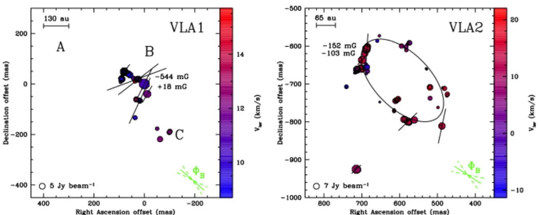
Fig. 1.Close-up view of the 22 GHz H2O maser features detected around the radio source VLA 1 (left panel) and VLA 2 (right panel). The
reference position isα2000 = 20h38m36.s435 andδ2000 = 42◦3734.84 (see Sect.2). The octagonal symbols are the identified maser features
in the present work scaled logarithmically according to their peak flux density (TablesA.1andA.2). The linear polarization vectors, scaled logarithmically according to polarization fractionPl, are overplotted. In the bottom-right corner of both panels the error-weighted orientation of
the magnetic field (ΦB, see Sect.3) is also reported; the two dashed segments indicate the uncertainties. The ellipse drawn in the right panel is the
result of the best fit of the H2O masers detected in the present work (epoch 2012.54). Its parameters are listed in Table1. The estimated values of
the magnetic field strength are also shown in both panels next to the corresponding H2O maser.
S11 analyzed the polarized emission of 22 GHz H2O masers and
found that the magnetic field around VLA 1 and VLA 2 (sepa-rated by just 1300 AU) has different orientation and strength.
Therefore, we propose W75N(B) as the best case known where the transition from a non-collimated to a well-collimated outflow in the very early phase of HMSF can be observed in “real time”. In this letter, we present new polarimetric VLBI ob-servations of H2O masers to confirm the elliptical expansion of
the shell-like structure around VLA 2 as well as to determine possible changes in the magnetic field.
2. Observations and analysis
The star-forming region W75N(B) was observed in the 616−523
transition of H2O (rest frequency: 22.23508 GHz) with the
NRAO1 VLBA on July 15, 2012. The observations were made in full polarization mode using a bandwidth of 4 MHz to cover a velocity range of∼54 km s−1. The data were correlated with
the DiFX correlator using 2000 channels and generating all four polarization combinations (RR, LL, RL, LR) with a spectral res-olution of 2 kHz (∼0.03 km s−1). Including the overheads, the
total observation time was 8 h.
The data were calibrated using AIPS by following the same calibration procedure described in S11. We used the same cal-ibrator used by S11, i.e., J2202+4216. Then we imaged theI,
Q,U, andVcubes (rms=21 mJy beam−1) using the AIPS task
IMAGR (beam size 0.87 mas×0.61 mas, PA = +3.75◦). The
QandU cubes were combined to produce cubes of polarized intensity (POLI) and polarization angle (χ). Because W75N(B) was observed 11 days after a POLCAL observations run made by NRAO2, we calibrated the linear polarization angles of the H2O masers by comparing the linear polarization angle of
J2202+4216 that we measured with the angles measured dur-ing that POLCAL observations run (χJ2202+4216 =−15◦.0±0◦.3).
The formal errors onχ are due to thermal noise. This error is given byσχ = 0.5σP/P×180◦/π(Wardle & Kronberg1974), wherePandσPare the polarization intensity and corresponding rms error, respectively. We estimated the absolute position of 1 The National Radio Astronomy Observatory (NRAO) is a facility of
the National Science Foundation operated under cooperative agreement by Associated Universities, Inc.
2 http://www.aoc.nrao.edu/~smyers/calibration/
the brightest maser feature through fringe rate mapping by us-ing the AIPS task FRMAP. As the formal errors of FRMAP are Δα = 2.6 mas andΔδ =1.2 mas, the absolute position uncer-tainty will be dominated by the phase fluctuations. We estimate these to be on the order of no more than a few mas from our ex-perience with other experiments and varying the task parameters. We analyzed the polarimetric data following the procedure reported in S11. First, we identified the H2O maser features
and determined the linear polarization fraction (Pl) and χ for
each identified H2O maser feature. Second, we used the full
ra-diative transfer method (FRTM) code for 22 GHz H2O masers
(Vlemmings et al. 2006; Appendix A). The output of this code provides estimates of the emerging brightness tempera-ture (TbΔΩ) and of the intrinsic thermal linewidth (ΔVi). From
TbΔΩandPl, we then determined the angle between the maser
propagation direction and the magnetic field (θ). Ifθ > θcrit =
55◦ the magnetic field appears to be perpendicular to the lin-ear polarization vectors; otherwise, it is parallel (Goldreich et al. 1973). Finally, the best estimates ofTbΔΩandΔViare included
in the FRTM code to produce the I and V models used for measuring the Zeeman splitting (see AppendixA).
3. Results
3.1. VLA 1
The H2O masers in VLA 1 are distributed along the
ra-dio jet as previously observed by T03 (epoch 1999.25), S11 (epoch 2005.89), and K13 (epoch 2007.41). Surcis et al. (2011) found the H2O masers clustered in three groups, named A, B,
and C. In this work (epoch 2012.54), we detected 38 H2O masers
(named VLA1.01 – VLA1.38; TableA.1 in groups B and C, but not in A (Fig.1). Group A was also not detected in 1999 and 2007. For a detailed comparison of the H2O maser
parame-ters measured in epochs 2005.89 and 2012.54 see TableA.3. We detected linearly polarized emission from seven H2O masers (Pl = 0.6%−4.5%), and the error-weighted
linear polarization angle is χ VLA1 = −41◦ ± 15◦. The
FRTM code was able to fit four out of the seven H2O masers
(Table A.1). Because the lower limit of the fitting range of TbΔΩ is 106 K sr, the estimated values of ΔVi and
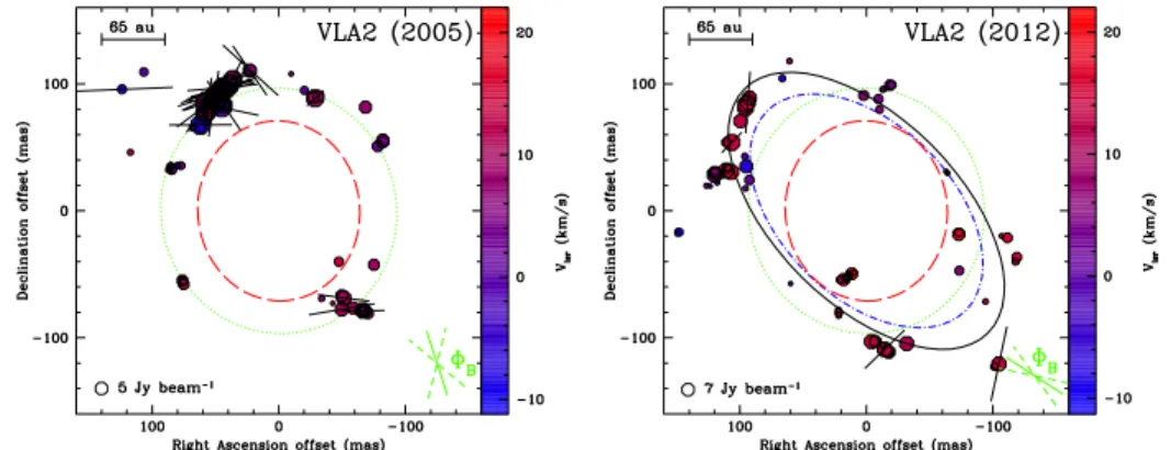
Fig. 2.Comparison of the H2O masers around VLA 2 in epoch 2005.89 (left panel; S11) and in epoch 2012.54 (right panel; present work). A
comparison of the elliptical fits of the H2O maser distributions observed in the past 13 years is also shown (see Fig.1for more details). The maser
LSR radial velocity baron the right of both panelsshows the same velocity range. Four ellipses are drawn, which are assumed to have the same center (the (0, 0) reference position). They are the results of the best fit of the H2O masers detected by T03 (epoch 1999.25; red dashed ellipse), S11
(epoch 2005.89; green dotted ellipse), K13 (epoch 2007.41; blue dot-dashed ellipse), and the present work (epoch 2012.54; black solid ellipse). Their parameters are listed in Table1.
and θVLA1 = +90◦+10 ◦
−10◦. This implies that the magnetic
field is perpendicular to the linear polarization vectors and the error-weighted orientation on the plane of the sky is
ΦB VLA1= +49◦±15◦. The foreground, ambient, and internal
Faraday rotations are small or negligible as shown by S11. Circularly polarized emission is detected in VLA1.06 (PV = 0.07%) and VLA1.12 (1.8%). Because the FRTM code was not able to determineTbΔΩandΔVi for VLA1.12, we considered
the values of the closest maser VLA1.10 to produce theIandV
models (Fig.A.1). The estimated magnetic field strengths along the line of sight (B||) are+18 mG and –544 mG (a negative mag-netic field strength indicates that the magmag-netic field is pointing towards the observer; otherwise away from the observer). The magnetic field strength B is related to B|| by B|| = B cosθ if
θ ±90◦. BecauseθVLA1 = 90◦+10 ◦
−10◦, we can only provide a
lower limit ofBfor VLA 1 (TableA.3).
3.2. VLA 2
We detected 68 H2O masers (named VLA2.01–VLA2.68;
TableA.2) showing an elliptical distribution similar to that ob-served in epoch 2007.41 (K13). An elliptical fit reveals that the semi-major axis (a) and the semi-minor axis (b) are 136±4 mas and 73±2 mas, respectively, and the position angle is PA = 45◦±2◦. The center of the ellipse is at the positioncα= +593±
2 mas,cδ=−690±3 mas with respect to VLA1.06. The eccen-tricity,e= 1−(b/a)2, of the fitted ellipse is 0.84±0.05.
Five H2O masers show linearly polarized emission (Pl =
0.7%–1.6%), and the error-weighted linear polarization angle is
χ VLA2 = −33◦ ±21◦. The FRTM code was able to properly
fit only VLA2.64 and the outputs areΔVi,VLA2 = 1.98 km s−1,
TbΔΩVLA2 =6×10⁸ K sr, andθVLA2 = +84◦+6 ◦
−10◦. This implies
that the magnetic field is perpendicular to the linear polarization vectors and the error-weighted orientation on the plane of the sky isΦB VLA2= +57◦±21◦.
Circularly polarized emission was detected towards two H2O masers, namely VLA2.44 (PV =0.7%) and VLA2.48 (PV =0.4%). These masers do not show linear polarization and consequently no information on ΔVi and TbΔΩ is available. To measure the magnetic field strength, we decided to assign values to ΔVi andTbΔΩthat could produce the best I andV fitting models. These areΔVi =2.0 km s−1for both masers, and
TbΔΩ = 5×10⁹K sr andTbΔΩ = 109K sr for VLA2.44 and
VLA2.48, respectively. The goodness of the fit can be seen in Fig.A.1. The estimatedB||are –152 mG and –103 mG.
4. Discussion
4.1. The immutable VLA 1
The H2O masers in VLA 1 show a linear distribution (PA≈43◦)
persistent over 13 years. Nevertheless, there are minor differ-ences compared to S11. Specifically, the flux density has gen-erally decreased from 2005 to 2012 (TableA.3). This may ex-plain the disappearance of the masers of group A, which also had largerVlsrthan groups B and C and thus they were
proba-bly tracing an occasional fast ejection event (VVLA 1
lsr =9 km s− 1,
Carrasco-González et al.2010). The inferred magnetic field in VLA 1 is along the radio jet and it is almost aligned with the large-scale CO-outflow (PAout = 66◦; Hunter et al. 1994), as
measured in 2005 (TableA.3).
The stability of the maser and magnetic field distribution around VLA 1 might indicate a relatively evolved stage of this massive YSO in comparison with VLA 2 (see below).
4.2. The evolution of the expanding H2O maser shell in VLA 2
Unlikely VLA 1, VLA 2 has shown remarkable evolution both in structure and magnetic field in the last decade, as probed by the H2O masers mapped with VLBI at four different epochs. In
all epochs, the H2O masers have shown a different distribution
around VLA 2, in size and/or shape, going from circular (T03, S11) to elliptical (K13, present work; Fig.2and Table1).
In epoch 1999.25, the elliptical fit reveals that a and b
have almost the same value (e = 0.43 ±0.01, Table 1) in-dicating that the H2O masers are tracing an almost circular
shell-like structure (T03). This shell is thought to be the sig-nature of a shock caused by the expansion of a non-collimated outflow; T03 also measured the proper motion of the individ-ual H2O masers, concluding that they are moving outward from
VLA 2 at∼19 km s−1.
In epoch 2005.89, S11 found that the circular shell increased its size by about 30 mas, but it did not changed its shape signif-icantly (e = 0.28±0.02). In about six years the circular shell expanded with a velocity of 24±3 km s−1that is consistent with
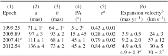
Table 1.Comparison of the fitted parameters of the ellipses from K13 (1999.25, 2005.89, 2007.41) and the present work (2012.54).
(1) (2) (3) (4) (5) (6)
Epoch a b PA ea Expansion velocityb
(mas) (mas) (◦) (mas yr−1) (km s−1)
1999.25 71±1c 64±1c 5±3c 0.43±0.01
2005.89 97±3 93±2 15±45 0.28±0.02 3.9±0.5 24±3 2007.41c 111±1 68±1 45±1 0.79±0.02 9.2±2.0 57±12 2012.54 136±4 73±2 45±2 0.84±0.05 4.9±0.8 30±5 4.9±0.3d 30±2d
Notes.(a)Eccentricity,e= 1−(b/a)2.(b)From the difference in the
semi-major axis size of the ellipse between different epochs (1999.25– 2005.89; 2005.89–2007.41; 2007.41–2012.54). (c) The considered
epoch is May 29, 2007.(d)Between epoch 1999.25 and epoch 2012.54.
suggests that the formation of an early non-collimated outflow from a massive YSO is observed at mas scale; S11 also deter-mined that the magnetic field is of the order of 1–2 G around VLA 2 and it is oriented alonga.
After only two years from the observations of S11, K13 ob-served that the H2O maser shell is still expanding, but along a
more dominant axis with PA = +45◦±1◦ (e = 0.79±0.02). The increment of the ellipticity could be the sign of the launch-ing of a collimated jet that overtakes the non-collimated outflow. Surprisingly, the shell is now aligned with both the thermal radio jet and the magnetic field in VLA 1.
Our observations of epoch 2012.54 show that the expansion of the shell still continues after five years and that its ellipticity has increased (e = 0.84±0.02). The position angle of our fit is equal to that determined by K13 indicating that the supposed launching of a collimated jet has actually happened (Table1).
In contrast to the magnetic field in VLA 1, the magnetic field in VLA 2 has changed its orientation substantially (Fig.2). The magnetic field has rotated by about+40◦during the past seven years and it is now aligned with the major axis of the fitted ellipse of epoch 2012.54 (PA = +45◦±2◦). By comparingΦB VLA2
withΦB VLA1, we notice that the magnetic fields around VLA 2
and VLA 1 are now aligned with both the jet in VLA 1 and the el-liptical H2O maser shell in VLA 2. This configuration may arise
if the large-scale magnetic field of W75N(B) drives the orienta-tion of the two jets and potentially regulates HMSF as suggested by recent observations (Girart et al.2009; Tan et al.2013). A test of this hypothesis may be to determine the morphology of the magnetic field of the region at large scale via dust polariza-tion observapolariza-tions. Incidentally, we note that the inferred mag-netic field direction also appears to be perpendicular to the fil-amentary core and its velocity gradient traced by NH3 thermal
emission (Carrasco-González et al.2010).
A possible physical framework to explain our results in VLA 2 may be provided by recent MHD simulations (Seifried et al. 2012). In this context, the magnetic pressure drives a slow non-collimated outflow in the very first phase of protostel-lar formation. Immediately after the formation of a Keplerian disk, a short-lived fast and collimated jet overtakes the slow out-flow. This could be qualitatively in agreement with our findings in VLA 2.
In addition, a comparison between |B|||2005VLA2.89 = 345 mG and |B|||2012VLA2.54 = 128 mG shows that the magnetic field in epoch 2012.54 is one third of the magnetic field measured in
epoch 2005.89. The masers at the two epochs probe different gas properties and the measured variation of the magnetic field could simply be a consequence of it. We thus speculate that the variation may be due to the launching of the fast jet, but present simulations do not include the variation of the magnetic field strength during the early outflow evolution to corroborate our hypothesis.
From an observational perspective, to confirm our sce-nario it is necessary to monitor the expanding motion of the 22 GHz H2O maser structure and the magnetic field evolution
in the region over time. Furthermore, the determination of the 3D velocity structure of the outflow obtained with new proper motion measurements of the H2O masers and of the evolution of
the continuum morphology of VLA 2 will likewise be important.
5. Conclusions
We observed the massive star-forming region W75N(B) with the VLBA to detect linearly and circularly polarized emission from 22 GHz H2O masers associated with the two radio sources
VLA 1 and VLA 2. We observed that while the H2O maser
dis-tribution and the magnetic field around VLA 1 have not changed since 2005, the shell structure of the masers around VLA 2 is still expanding and increasing its ellipticity. Furthermore, the magnetic field around VLA 2 has changed its orientation accord-ing to the new direction of the major-axis of the shell-like struc-ture and it is now aligned with the magnetic field in VLA 1. We conclude that the H2O masers around VLA 2 are tracing the
evolution from a non-collimated to a collimated outflow.
Acknowledgements. We wish to thank an anonymous referee for making use-ful suggestions that have improved the paper. G.S. thanks Dr. D. Seifried for the useful discussion. J.M.T. acknowledges support from MICINN (Spain) grant AYA2011-30228-C03 (co-funded with FEDER funds). The ICC (UB) is a CSIC-Associated Unit through the ICE (CSIC). Sc acknowledges support of DGAPA, UNAM, and CONACyT (México).
References
Anderson, N., & Watson, W. D. 1993, ApJ, 407, 620
Baart, E. E., Cohen, R. J., Davies, R. D., et al. 1986, MNRAS, 219, 145 Banerjee, R., & Pudritz, R. E. 2007, ApJ, 660, 479
Beuther, H., & Shepherd, D. 2005, Astrophys. Space Sci. Lib., 324, 105 Carrasco-González, C., Rodríguez, L. F., Torrelles, J. M., et al. 2010, AJ, 139,
2433
Girart, J. M., Berltrán, M. T., Zhang, Q., et al. 2009, Science, 324, 1408 Goddi, C., Moscadelli, L., Alef, W., et al. 2005, A&A, 432, 161 Goldreich, P., Keeley, D. A., & Kwan, J. Y. 1973, ApJ, 179, 111 Hunter, T. R., Taylor, G. B., Felli, M., et al. 1994, A&A, 284, 215 Kim, J.-S., Kim, S.-W., Kurayama, T. et al. 2013, ApJ, 767, 86 (K13) Moscadelli, L., Goddi, C., Cesaroni, R., et al. 2007, A&A, 472, 867 Nedoluha, G. E., & Watson, W. D. 1991, ApJ, 367, L63
Nedoluha, G. E., & Watson, W. D. 1992, ApJ, 384, 185 Rygl, K., Brunthaler, A., Sanna, A., et al. 2012, A&A, 539, A79 Sanna, A., Moscadelli, L., Cesaroni, R., et al. 2010, A&A, 517, A78 Seifried, D., Banerjee, R., Klessen, R. S., et al. 2011, MNRAS, 417, 1054 Seifried, D., Pudritz, R. E., Banerjee, R., et al. 2012, MNRAS, 422, 347 Surcis, G., Vlemmings, W. H. T., Dodson, R., et al. 2009, A&A, 506, 757 Surcis, G., Vlemmings, W. H. T., Curiel, S., et al. 2011, A&A, 527, A48 (S11) Tan, J. C., Kong, A. K., Butler, M. J., et al. 2013, ApJ, 779, 96
Torrelles, J. M., Gómez, J. F., Rodríguez, L. F., et al. 1997, ApJ, 489, 744 Torrelles, J. M., Patel, N. A. Anglada, G., et al. 2003, ApJ, 598, L115 (T03) Vlemmings, W. H. T., Diamond, P. J., van Langevelde, H. J., et al. 2006, A&A,
448, 597
Wardle, J. F. C., & Kronberg, P. P. 1974, ApJ, 194, 249 Zinnecker, H., & Yorke, H. W. 2007, ARA&A, 45, 481
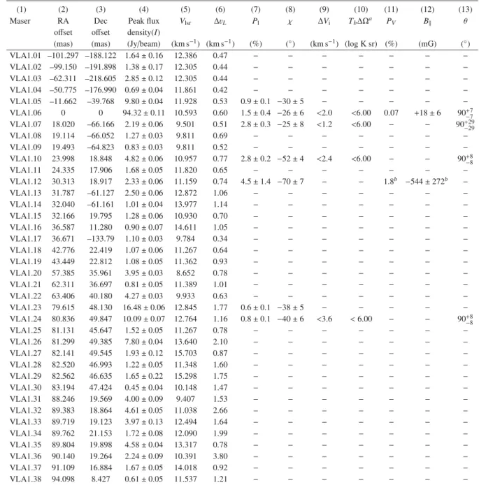
Table A.1.All 22 GHz H2O maser features detected around VLA 1 (epoch 2012.54).
(1) (2) (3) (4) (5) (6) (7) (8) (9) (10) (11) (12) (13)
Maser RA Dec Peak flux Vlsr ΔvL Pl χ ΔVi TbΔΩa PV B|| θ
offset offset density(I)
(mas) (mas) (Jy/beam) (km s−1) (km s−1) (%) (◦) (km s−1) (log K sr) (%) (mG) (◦) VLA1.01 –101.297 –188.122 1.64±0.16 12.386 0.47 − − − − − − − VLA1.02 –99.150 –191.898 1.38±0.17 12.305 0.44 − − − − − − − VLA1.03 –62.311 –218.605 2.85±0.12 12.305 0.44 − − − − − − − VLA1.04 –50.775 –176.990 0.69±0.04 11.861 0.42 − − − − − − − VLA1.05 –11.662 –39.768 9.80±0.04 11.928 0.53 0.9±0.1 −30±5 − − − − − VLA1.06 0 0 94.32±0.11 10.593 0.60 1.5±0.4 −26±6 <2.0 <6.00 0.07 +18±6 90+7
−7 VLA1.07 18.020 –66.166 2.19±0.06 9.501 0.51 2.8±0.3 −25±8 <1.2 <6.00 − − 90+29 −29 VLA1.08 19.114 –66.052 1.27±0.03 9.811 0.69 − − − − − − − VLA1.09 19.493 –64.823 0.83±0.03 9.811 0.52 − − − − − − − VLA1.10 23.998 18.848 4.82±0.06 10.957 0.77 2.8±0.2 −52±4 <2.4 <6.00 − − 90+−88 VLA1.11 24.335 17.906 1.68±0.05 11.820 0.65 − − − − − − − VLA1.12 30.313 18.917 2.33±0.06 11.159 0.74 4.5±1.4 −70±7 − − 1.8b −544±272b −
VLA1.13 31.787 –61.127 2.50±0.06 12.872 1.06 − − − − − − − VLA1.14 32.040 –61.161 1.01±0.04 13.977 1.14 − − − − − − − VLA1.15 32.166 19.795 1.28±0.06 10.930 0.70 − − − − − − − VLA1.16 36.587 11.280 0.90±0.07 14.611 1.05 − − − − − − − VLA1.17 36.671 –133.79 1.10±0.03 9.784 0.34 − − − − − − − VLA1.18 42.776 22.419 1.07±0.06 11.267 0.64 − − − − − − − VLA1.19 43.449 22.812 1.08±0.05 11.362 0.93 − − − − − − −
VLA1.20 57.385 35.961 3.95±0.03 8.652 0.78 − − − − − − −
VLA1.21 62.311 36.697 0.81±0.05 11.389 1.01 − − − − − − −
VLA1.22 63.406 40.180 4.27±0.03 9.933 0.63 − − − − − − −
VLA1.23 79.615 48.130 16.48±0.06 12.845 1.77 0.6±0.1 −38±5 − − − − − VLA1.24 80.836 49.847 10.09±0.07 12.764 1.16 0.8±0.1 −40±6 <3.6 <6.00 − − 90+8
−8 VLA1.25 81.131 45.647 1.52±0.05 11.267 0.78 − − − − − − − VLA1.26 81.299 49.385 7.80±0.04 13.640 2.10 − − − − − − − VLA1.27 82.141 49.545 1.93±0.12 15.703 0.87 − − − − − − − VLA1.28 82.520 46.993 1.22±0.05 11.348 1.60 − − − − − − − VLA1.29 82.562 46.635 1.65±0.22 15.298 1.75 − − − − − − − VLA1.30 83.194 47.424 0.45±0.04 10.148 1.47 − − − − − − −
VLA1.31 88.246 19.569 4.00±0.09 9.407 1.53 − − − − − − −
VLA1.32 89.383 18.864 4.61±0.05 11.038 2.66 − − − − − − − VLA1.33 89.719 19.123 3.97±0.13 12.494 1.64 − − − − − − − VLA1.34 89.762 21.153 1.72±0.08 12.090 1.99 − − − − − − − VLA1.35 89.804 19.898 4.58±0.04 13.317 0.78 − − − − − − − VLA1.36 90.140 19.264 2.24±0.09 10.391 3.80 − − − − − − − VLA1.37 91.109 16.884 1.67±0.05 14.018 0.92 − − − − − − −
VLA1.38 94.098 8.427 0.61±0.05 11.537 1.21 − − − − − − −
Notes.(a) The outputT
bΔΩmust be adjusted according to the real value ofΓ + Γν, which depends on the gas temperature (T). UsingΔVi ≈
0.5 (T/100)1/2(Vlemmings et al.2006) we estimated thatT
VLA1<2300 K for whichTbΔΩhas to be adjusted by adding at most+1.11 log K sr
(Anderson & Watson1993).(b)In the fitting model we include the valuesT
bΔΩ =1×10⁶K sr andΔVi=2.4 km s−1that are the estimated upper
limits of VLA1.10 (see Fig.A.1).
Appendix A: Measured and calculated physical parameters of the H2O masers
In TablesA.1andA.2we list all the H2O maser features detected
towards the two YSOs, VLA 1 and VLA 2, respectively. The tables are organized as follows. The name of the feature is re-ported in Col. 1. The positions, Cols. 2 and 3, refer to the bright-est H2O maser feature VLA1.06 that was used to self-calibrate
the data. We estimated the absolute position of VLA1.06 to be
α2000 = 20h38m36s.435 andδ2000 = 42◦3734.84 (see Sect.2).
The peak flux density (I), the LSR velocity (Vlsr), and the
FWHM (ΔvL) of the total intensity spectra of the maser
fea-tures are reported in Cols. 4–6, respectively;I,Vlsr, andΔvLare
obtained using a Gaussian fit. The mean linear polarization frac-tion (Pl) and the mean linear polarization angles (χ) are instead
reported in Cols. 8 and 9, respectively. We determinedPlandχ
of each H2O maser feature by only considering the consecutive
channels (more than two) across the total intensity spectrum for which the polarized intensity is≥5σ.
Fig. A.1.Total intensity spectra (I,upper panel) and circular polarization intensity spectra (V,lower panel) for the H2O masers VLA1.06, VLA1.12,
VLA2.44, and VLA2.48 (see TablesA.1andA.2). The thick red line is the best-fit models ofIandV emission obtained using the full radiative transfer method code for 22 GHz H2O masers. The maser features were centered on zero velocity.
FRTM code (Vlemmings et al.2006) that is based on the model for 22 GHz H2O maser of Nedoluha & Watson (1992), for which
the shapes of the total intensity, linear polarization, and circu-lar pocircu-larization spectra depend onTbΔΩ and ΔVi (Nedoluha
& Watson 1991, 1992). We model the observed linear polar-ized and total intensity maser spectra by griddingΔVibetween 0.4 km s−1and 4.0 km s−1, in steps of 0.025 km s−1, using a least-squares fitting routine (χ2-model) with 106 K sr < T
bΔΩ < 1011 K sr. We also set in our fit (Γ + Γ
ν) = 1 s−1, whereΓ is
the maser decay rate andΓν is the cross-relaxation rate for the
magnetic substated (see Vlemmings et al.2006and S11 for more details).
From the maser theory we know thatPl of the H2O maser
emission depends on the degree of its saturation and the angle between the maser propagation direction and the magnetic field (θ; e.g., Goldreich et al. 1973). Because TbΔΩ determines the relation betweenPlandθ, from the outputs of the FRTM code
we are able to estimate the anglesθthat are reported in Col. 13. The errors ofTbΔΩ,ΔVi, andθare determined by analyzing the
full probability distribution function.
Finally, the best estimates ofTbΔΩandΔViare then included
in the FRTM code to produce theI andVmodels that are used
for fitting the total intensity and circular polarized spectra of the H2O masers (see Fig.A.1). The magnetic field strength along
the line of sight, which is reported in Col. 12, is finally evaluated by using the equation
B||=Bcosθ= PVΔvL
2·AF−F
, (A.1)
whereΔvLis the FWHM of the total intensity spectrum,PV = (Vmax−Vmax)/Imaxis the circular polarization fraction (Col. 11),
and the AF−F coefficient, which depends on TbΔΩ, describes the relation between the circular polarization and the magnetic field strength for a transition between a high (F) and low (F) rotational energy level (Vlemmings et al.2006).
In Table A.3 we compare the parameters of the 22 GHz H2O masers detected around VLA 1 and VLA 2
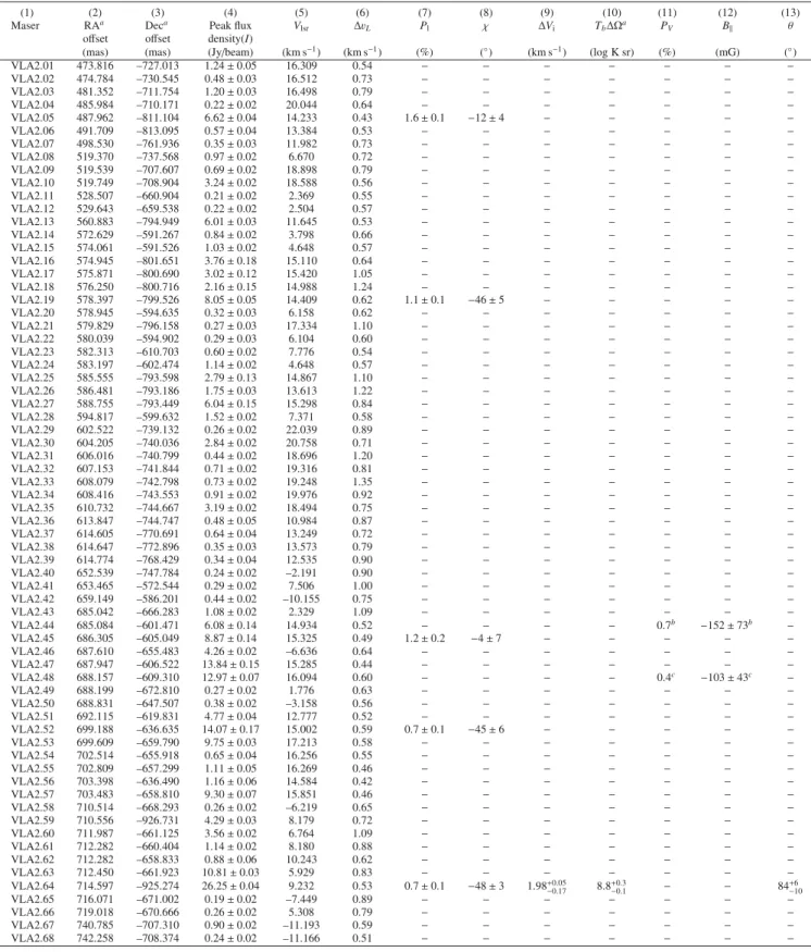
Table A.2.All 22 GHz H2O maser features detected around VLA 2 (epoch 2012.54).
(1) (2) (3) (4) (5) (6) (7) (8) (9) (10) (11) (12) (13)
Maser RAa Deca Peak flux V
lsr ΔvL Pl χ ΔVi TbΔΩa PV B|| θ offset offset density(I)
(mas) (mas) (Jy/beam) (km s−1) (km s−1) (%) (◦) (km s−1) (log K sr) (%) (mG) (◦)
VLA2.01 473.816 –727.013 1.24±0.05 16.309 0.54 − − − − − − −
VLA2.02 474.784 –730.545 0.48±0.03 16.512 0.73 − − − − − − −
VLA2.03 481.352 –711.754 1.20±0.03 16.498 0.79 − − − − − − −
VLA2.04 485.984 –710.171 0.22±0.02 20.044 0.64 − − − − − − −
VLA2.05 487.962 –811.104 6.62±0.04 14.233 0.43 1.6±0.1 −12±4 − − − − −
VLA2.06 491.709 –813.095 0.57±0.04 13.384 0.53 − − − − − − −
VLA2.07 498.530 –761.936 0.35±0.03 11.982 0.73 − − − − − − −
VLA2.08 519.370 –737.568 0.97±0.02 6.670 0.72 − − − − − − −
VLA2.09 519.539 –707.607 0.69±0.02 18.898 0.79 − − − − − − −
VLA2.10 519.749 –708.904 3.24±0.02 18.588 0.56 − − − − − − −
VLA2.11 528.507 –660.904 0.21±0.02 2.369 0.55 − − − − − − −
VLA2.12 529.643 –659.538 0.22±0.02 2.504 0.57 − − − − − − −
VLA2.13 560.883 –794.949 6.01±0.03 11.645 0.53 − − − − − − −
VLA2.14 572.629 –591.267 0.84±0.02 3.798 0.66 − − − − − − −
VLA2.15 574.061 –591.526 1.03±0.02 4.648 0.57 − − − − − − −
VLA2.16 574.945 –801.651 3.76±0.18 15.110 0.64 − − − − − − −
VLA2.17 575.871 –800.690 3.02±0.12 15.420 1.05 − − − − − − −
VLA2.18 576.250 –800.716 2.16±0.15 14.988 1.24 − − − − − − −
VLA2.19 578.397 –799.526 8.05±0.05 14.409 0.62 1.1±0.1 −46±5 − − − − −
VLA2.20 578.945 –594.635 0.32±0.03 6.158 0.62 − − − − − − −
VLA2.21 579.829 –796.158 0.27±0.03 17.334 1.10 − − − − − − −
VLA2.22 580.039 –594.902 0.29±0.03 6.104 0.60 − − − − − − −
VLA2.23 582.313 –610.703 0.60±0.02 7.776 0.54 − − − − − − −
VLA2.24 583.197 –602.474 1.14±0.02 4.648 0.57 − − − − − − −
VLA2.25 585.555 –793.598 2.79±0.13 14.867 1.10 − − − − − − −
VLA2.26 586.481 –793.186 1.75±0.03 13.613 1.22 − − − − − − −
VLA2.27 588.755 –793.449 6.04±0.15 15.298 0.84 − − − − − − −
VLA2.28 594.817 –599.632 1.52±0.02 7.371 0.58 − − − − − − −
VLA2.29 602.522 –739.132 0.26±0.02 22.039 0.89 − − − − − − −
VLA2.30 604.205 –740.036 2.84±0.02 20.758 0.71 − − − − − − −
VLA2.31 606.016 –740.799 0.44±0.02 18.696 1.20 − − − − − − −
VLA2.32 607.153 –741.844 0.71±0.02 19.316 0.81 − − − − − − −
VLA2.33 608.079 –742.798 0.73±0.02 19.248 1.35 − − − − − − −
VLA2.34 608.416 –743.553 0.91±0.02 19.976 0.92 − − − − − − −
VLA2.35 610.732 –744.667 3.19±0.02 18.494 0.75 − − − − − − −
VLA2.36 613.847 –744.747 0.48±0.05 10.984 0.87 − − − − − − −
VLA2.37 614.605 –770.691 0.64±0.04 13.249 0.72 − − − − − − −
VLA2.38 614.647 –772.896 0.35±0.03 13.573 0.79 − − − − − − −
VLA2.39 614.774 –768.429 0.34±0.04 12.535 0.90 − − − − − − −
VLA2.40 652.539 –747.784 0.24±0.02 –2.191 0.90 − − − − − − −
VLA2.41 653.465 –572.544 0.29±0.02 7.506 1.00 − − − − − − −
VLA2.42 659.149 –586.201 0.44±0.02 –10.155 0.75 − − − − − − −
VLA2.43 685.042 –666.283 1.08±0.02 2.329 1.09 − − − − − − −
VLA2.44 685.084 –601.471 6.08±0.14 14.934 0.52 − − − − 0.7b −152±73b −
VLA2.45 686.305 –605.049 8.87±0.14 15.325 0.49 1.2±0.2 −4±7 − − − − −
VLA2.46 687.610 –655.483 4.26±0.02 –6.636 0.64 − − − − − − −
VLA2.47 687.947 –606.522 13.84±0.15 15.285 0.44 − − − − − − −
VLA2.48 688.157 –609.310 12.97±0.07 16.094 0.60 − − − − 0.4c −103±43c −
VLA2.49 688.199 –672.810 0.27±0.02 1.776 0.63 − − − − − − −
VLA2.50 688.831 –647.507 0.38±0.02 –3.158 0.56 − − − − − − −
VLA2.51 692.115 –619.831 4.77±0.04 12.777 0.52 − − − − − − −
VLA2.52 699.188 –636.635 14.07±0.17 15.002 0.59 0.7±0.1 −45±6 − − − − −
VLA2.53 699.609 –659.790 9.75±0.03 17.213 0.58 − − − − − − −
VLA2.54 702.514 –655.918 0.65±0.04 16.256 0.55 − − − − − − −
VLA2.55 702.809 –657.299 1.11±0.05 16.269 0.46 − − − − − − −
VLA2.56 703.398 –636.490 1.16±0.06 14.584 0.42 − − − − − − −
VLA2.57 703.483 –658.810 9.30±0.07 15.851 0.46 − − − − − − −
VLA2.58 710.514 –668.293 0.26±0.02 –6.219 0.65 − − − − − − −
VLA2.59 710.556 –926.731 4.29±0.03 8.179 0.72 − − − − − − −
VLA2.60 711.987 –661.125 3.56±0.02 6.764 1.09 − − − − − − −
VLA2.61 712.282 –660.404 1.14±0.02 8.180 0.88 − − − − − − −
VLA2.62 712.282 –658.833 0.88±0.06 10.243 0.62 − − − − − − −
VLA2.63 712.450 –661.923 10.81±0.03 5.929 0.83 − − − − − − −
VLA2.64 714.597 –925.274 26.25±0.04 9.232 0.53 0.7±0.1 −48±3 1.98+0.05
−0.17 8.8−+00..31 − − 84+−610
VLA2.65 716.071 –671.002 0.19±0.02 –7.449 0.89 − − − − − − −
VLA2.66 719.018 –670.666 0.26±0.02 5.308 0.79 − − − − − − −
VLA2.67 740.785 –707.310 0.90±0.02 –11.193 0.59 − − − − − − −
VLA2.68 742.258 –708.374 0.24±0.02 –11.166 0.51 − − − − − − −
Notes.(a) The outputT
bΔΩmust be adjusted according to the real value ofΓ + Γν, which depends on the gas temperature (T). UsingΔVi ≈
0.5 (T/100)1/2 (Vlemmings et al.2006) we estimated thatT
VLA 2 = 1600 K (Γ + Γν = 9 s−1) for whichTbΔΩhas to be adjusted by adding
+0.95 log K sr (Anderson & Watson1993).(b)In the fitting model we include the valuesT
bΔΩ =5×10⁹K sr andΔVi=2.0 km s−1.(c)In the
Table A.3.Comparison of 22 GHz H2O maser parameters between epochs 2005.89 (S11) and 2012.54 (this work).
Epoch 2005.89a Epoch 2012.54
VLA 1 VLA 2 VLA 1 VLA 2
Number of maser features 36 88 38 68
Vlsrrange (km s−1) [+8.1;+24.7] [−7.7;+14.8] [+9.4;+15.7] [−11.2;+22.0]
Irange (Jy beam−1) [0.13; 158.28] [0.09; 198.45] [0.45; 94.32] [0.19; 26.25]
Polarizationb
Plrange (%) [0.6; 25.7] [0.2; 6.1] [0.6; 4.5] [0.7; 1.6]
PVrange (%) [0.3; 4.2] [0.1; 3.0] [0.1; 1.8] [0.4; 0.7] Intrinsic characteristics
ΔVirange (km s−1) [0.6; 2.0] [0.7; 3.4] [1.2; 3.6] 2.0
TbΔΩrange (log K sr) [8.9; 10.7] [8.6; 10.7] [6.0; 6.0] 8.8
ΔVib(km s−1) 1.0−+00..82 2.5+ 0.6
−0.4 <2.4 2.0+ 0.1
−0.2
TbΔΩb(log K sr) 10.6−+01..15 9.4−+00..69 <6.0 8.8+−00..31
Td(K) 400 2500 <2300 1600
Γ + Γνd 3 14 <13 9
Magnetic field
χrange (◦) [−90;+58] [−90;+83] [−70;−25] [−48;−4]
θrange (◦) [+66;+90] [+61;+90] [+90;+90] +84 ΦBrange (◦) [−32; 0] [−7; 0] [+20;+65] [+42;+86]
|B|||range (mG) [54; 809] [38; 957] [18; 544] [103; 152]
χe(◦) −67±40 −72±32 −41±15 −33±21
θe(◦) +83+7
−15 +85+
6
−36 +90+
10
−10 +84+
6
−10
ΦB (◦) +23±40 +18±32 +49±15 +57±21
|B||| f(mG) 81±62 145±110 >18 116±35
|B| f,g(mG) 665±509 1663±1262 >104h 1110±335
Arithmetic mean of|B|||(mG) 264 345 281 128
Notes.(a)Parameters from S11.(b)Averaged values determined by analyzing the total full probability distribution function.(c)T≈100·(ΔV i/0.5)2
is the gas temperature of the region where the H2O masers arise.(d)Cross-relaxation rate. The values ofTbΔΩhave to be adjusted by adding
+0.48 (Γ + Γν=3),+0.95 (Γ + Γν=9),+1.11 (Γ + Γν=13),+1.15 (Γ + Γν=14) as described in Anderson & Watson (1993).(e)Error-weighted values, where the weights arewi =1/eiandei is the error of theith measurements.(f)Error-weighted values, where the weights arewi =1/e2i.
(g)|B|=|B