DYNAMIC CRITICAL PROPERTIES OF DISORDERED MAGNETIC SYSTEMS
Zane V. Beckwith
A dissertation submitted to the faculty at the University of North Carolina at Chapel Hill in partial fulfillment of the requirements for the degree of Doctor of Philosophy in the
Department of Physics.
Chapel Hill 2014
Approved by:
Dmitri Khveshchenko Joaquin Drut
c
2014
ABSTRACT
Zane V. Beckwith: Dynamic Critical Properties of Disordered Magnetic Systems (Under the direction of Dmitri Khveshchenko)
TABLE OF CONTENTS
LIST OF TABLES . . . vi
LIST OF FIGURES . . . vii
LIST OF ABBREVIATIONS AND SYMBOLS . . . viii
1 INTRODUCTION . . . 1
2 BACKGROUND . . . 3
2.1 Avalanches. . . 3
2.2 Phase Transition . . . 4
2.3 Mean-field Description of Avalanche Phase Transition . . . 8
2.4 Universal Long-Distance Behavior and Minimal Models . . . 12
2.5 Universality in Three Dimensional Disordered Ising Models . . . 15
2.6 Relationship Between Random Fields and Random Bonds . . . 17
2.7 Irrelevant Variables and Hyperscaling Violation . . . 20
2.8 Anomalous Diffusion in Disordered Systems . . . 24
3 METHODS . . . 27
3.1 Ising Models . . . 27
3.2 Simulations . . . 31
3.4 Repetition and Averaging . . . 35
3.5 Finite-Size Scaling of Spanning Avalanche Numbers . . . 36
4 RESULTS . . . 43
4.1 Scaling of Avalanche Numbers . . . 43
4.2 Phase Diagram . . . 50
4.3 Critical Exponents . . . 52
5 DISCUSSION . . . 56
5.1 Universality . . . 56
5.2 Hyperscaling Violation in Ising Metastable Avalanches . . . 62
5.3 Indications of Anomalous Diffusion Processes. . . 64
6 CONCLUSIONS . . . 66
LIST OF TABLES
4.1 Final Estimates of Critical Parameters for Combined RBIM/RFIM . . . 52
LIST OF FIGURES
2.1 Distributions of Avalanche Sizes . . . 5
2.2 Magnetization Curves for Sub-critical and Super-critical RFIM . . . 7
3.1 1d Spanning Avalanche Numbers . . . 37
3.2 Scaled 1d Spanning Avalanche Numbers . . . 39
4.1 Scaling of Spanning Avalanche Numbers forσb = 0.0 . . . 44
4.2 Scaling of Spanning Avalanche Numbers forσb = 0.1 . . . 45
4.3 Scaling of Spanning Avalanche Numbers forσb = 0.3 . . . 46
4.4 Scaling of Spanning Avalanche Numbers forσb = 0.5 . . . 47
4.5 Scaling of Spanning Avalanche Numbers forσb = 0.9 . . . 48
4.6 Scaling of Spanning Avalanche Numbers forσf = 0.0 . . . 49
4.7 Phase Diagram of the Combined RBIM/RFIM . . . 51
4.8 Critical Exponents Along the Phase Boundary . . . 54
5.1 Shared Scaling of All Models, 1d Avalanches . . . 57
LIST OF ABBREVIATIONS AND SYMBOLS
RBIM Random-Bond Ising Model
RFIM Random-Field Ising Model
Si Spin at i’th site
Jij Bond between i’th andj’th spins
P
<ij> Sum over nearest-neighbor pairs only
σb Width of the Gaussian distribution from which the bonds in a RBIM are
chosen
σf Width of the Gaussian distribution from which the local fields in an RFIM
are chosen
σb,critical,σf,critical Critical values of the bond and field disorder, respectively
L Side length of the lattice of spins
Ni Number of avalanches observed during a magnetic field sweep, where i
denotes the type of avalanche (non-spanning, 1d spanning, 2d spanning, or 3d spanning)
RG Renormalization Group, a framework for understanding the behavior of systems near critical phase transitions
ξ Correlation length, defined as the distance over which fluctuations are correlated
ν Critical exponent giving the divergence of the correlation length as the critical point is approached: ξ ≈ σ−σc
σ
−ν
αL´evy Parameter controlling width and decay properties of functional fit to the
avalanche number distribution. Related to anomalous diffusion (αLevy´ <2 indicates a non-Gaussian distribution)
βL´evy Parameter controlling asymmetry of functional fit to the avalanche number
CHAPTER 1: INTRODUCTION
When natural systems are driven out of one stable state and into another, they often respond by jumping discontinuously through a cascade of intermediate non-equilibrium states, rather than with a smooth continuous motion. Think of a heavy box being pushed across a rough floor, or a tree limb cracking under a load. An excellent model to keep in mind when discussing these phenomena is of building a sandpile at the beach by slowly dropping sand on top of the pile. The sandpile maintains its shape for long periods, but changes suddenly when a portion collapses under its own weight.
These abrupt changes in response to a driving force are referred to as ‘avalanches’, in reference to the snow analogue of the sandpile model. Avalanches in the natural world have been the subject of scientific study for decades. One of the earliest-studied, and most dramatic, examples is an earthquake (Gutenberg and Richter, 1954): as the Earth’s continental plates shift under tectonic stress, they respond through abrupt, sometimes cataclysmic shifts that release huge amounts of energy. A more prosaic, but very important, example from materials science is Barkhausen noise: a ferromagnetic material placed in a time-dependent field will respond with a magnetization that does not vary smoothly in time but rather with large chunks of the material switching orientation abruptly (Durin and Zapperi,2006). In this case, the avalanches can be measured using an induction coil wrapped around the material, and the jumps can actually be heard as noise from a speaker connected to the coil. Similar avalanche behavior has also been observed in, for example, the structural phase transitions (‘martensitic transformations’) of certain materials (Carrillo et al., 1998), the depinning of vortices in superconductors (Field and Witt,1995), the sliding of charge-density waves (Middleton and Fisher,1993), and the ‘stair-step’ metamagnetic transformation of colossal magnetoresistance
Considering the wide variety of systems in which these avalanches appear, and the fact that their behavior is largely similar in all cases (Sornette,2003), a desire arises to understand what, if any, common mechanism describes their behavior. Avalanche phenomena generally occur in very complex systems with a large number of interacting constituents. Scientific models could never hope to fully describe such complex systems, but simple, minimal models have been found that exhibit the essential avalanche behavior. The present study will attempt to find such underlying commonality in these avalanche phenomena by studying a class of minimal models known as disordered Ising models. These models have been the subject of great interest for decades, and find application in fields as diverse as materials engineering (Belanger, 1998) to pattern formation in the brain (Paczuskiet al., 1996). Our interest will be in the rich avalanche behavior observed in these models over the past two decades (Sethna and Dahmen, 2001). The disordered Ising models comprise a diverse class of systems, so the study of commonality in avalanche behavior shared amongst them is a strong beginning to the study of such commonality in the avalanche behavior of all natural systems.
CHAPTER 2: BACKGROUND
Section 2.1: Avalanches
The avalanche phenomena discussed above have been studied in various ways for decades, and there are multiple simple models that can be used to simulate their behavior. One very popular paradigm for these studies is known as Self-Organized Criticality (SOC). In this view, the avalanches exhibit features characteristic of the theory of critical phase transitions, even though no parameters are available to tune the system to such a transition; the system has ‘self-organized’ itself into a critical state. Thus, SOC studies focus on simple models that have this parameter-free criticality; the sandpile model discussed above is the archetypal SOC model (Bak and Tang, 1987).
However, the connection of SOC studies to actual natural phenomena is a subject of great debate (Sornette, 2003, chapter 15). An alternate viewpoint studies models which a priori should have relevance to particular systems, and regards any critical-like behavior as most likely arising from an actual critical point1. A prominent example of this, motivated by
materials science concerns, is the avalanche behavior observed in a class of simple magnetic models, the Ising models. Ising models have been studied in physics for nearly a century (Ising, 1925), but it was not until much later that it was realized that the addition of randomness to
the models results in avalanche behavior much like that discussed above (Sethna et al., 1993; Vives and Planes, 1994).
What is meant by saying that the models exhibit behavior similar to observed phenomena? How are the models compared to natural behavior? The characteristic feature of natural
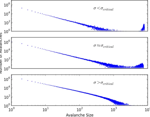
avalanches is the statistical distribution of their sizes; Fig. 2.1 shows an example size distribution, drawn from the Ising model avalanches observed in the present work. The definition of an avalanche’s size varies according to the system: for earthquakes it is the amount of energy released; for Barkhausen noise it is the jump in the magnetization; for a sandpile it is the amount of sand; for the Ising models it is the number of individual constituents, known as spins, involved in the transition. This is a rather unsophisticated comparison to make, but one should likely not expect more detailed agreement between such complex phenomena and such simple models. More importantly, though, the simplicity of the comparison is really the important point: the fact that so many natural phenomena and so many theoretical models exhibit this same, simple behavior (Sornette, 2003; Sethna and Dahmen, 2001) indicates that there is some very general mechanism at work. This issue will
be developed further in Section 2.4.
Section 2.2: Phase Transition
The most important feature of the distributions shown in Fig. 2.1 is their apparent power-law behavior; in all three log-log plots, the distributions are straight lines at small sizes. This is the most famous example of the critical behavior (a power-law admits no fundamental length scale, and such scale-free behavior is a hallmark of critical phenomena) discussed in the previous section. However, the middle plot (labeled ‘σ ≈σcritical’) is different from the
other two. In the top plot, the number of avalanches dies off beyond sizes of about 2×10³ (the avalanche size here means the number of spins that engage in the avalanche), with only a narrow peak popping up at very large sizes. In the bottom plot, this die-off behavior is more pronounced, exhibiting a clear exponential behavior at larger sizes. Only in the middle plot are avalanches present at all sizes2.
What are the differences in the systems represented by these three plots? They represent three different realizations of the randomized Ising models discussed in the previous section, with three different amounts of randomness. The parameter σ controls the amount of randomness in the system (Section 3.1 explains this concept more concretely), with σ = 0 corresponding to the standard, non-randomized, Ising model. Thus, when sweeping this parameter σ, the system transitions between two different types of behavior (from the lack of large avalanches except for an isolated peak at very large sizes in the top plot, to exponential decay of the avalanche distribution in the bottom plot in Fig. 2.1). Furthermore, at a parameter value (known as σcritical) intermediate between these two behaviors, the
system exhibits power-law behavior (the middle plot in Fig.2.1). This is the hallmark of a second-order phase transition!
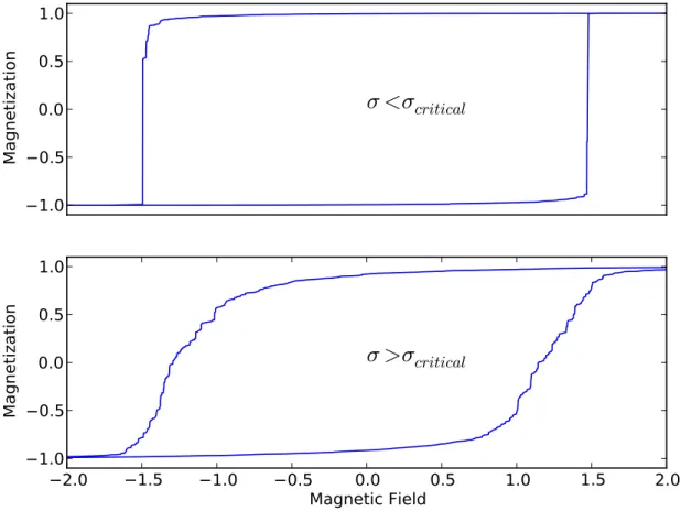
The physical meaning of this transition can be more clearly seen in the magnetization plots. As stated above, the Ising model is a model of a magnetic material, which means its magnetization may be measured; the magnetization corresponds to the number of spins that point in the same direction, and an avalanche causes a sharp change in the magnetization. Fig. 2.2shows representative magnetization plots for the cases σ < σcritical and σ > σcritical.
In these plots, all of the spins start off pointing in the negative direction (thus negative magnetization at the left end of the plot) and the system is driven by an increasing magnetic field, which progressively flips the spins to the positive direction (thus positive magnetization at the right end of the plot); the sweep is then reversed, going from positive to negative, and the fact that the behavior is not fully reversible leads to the hysteresis seen. In the case that σ > σcritical, randomness is high, each spin effectively has its own environment, and thus only
small clusters of spins will flip together. This gives a smooth magnetization curve and an avalanche size distribution that has only small avalanches. Conversely, when σ < σcritical,
2.0
1.5
1.0
0.5
0.0
0.5
1.0
1.5
2.0
Magnetic Field
1.0
0.5
0.0
0.5
1.0
Magnetization
σ >σ
critical
1.0
0.5
0.0
0.5
1.0
Magnetization
σ <σ
critical
change the magnetization drastically; this is the origin of the sharp bump at very large sizes in the avalanche size distribution.
Because this is a phase transition in a non-equilibrium system (we are driving the spins out of equilibrium with the magnetic field) between two different classes of dynamic behavior, this is an example of a non-equilibrium phase transition. For smallσ(including the usual pure Ising model) the system evolves primarily through a small number of very large avalanches. For large σ, on the other hand, the system evolves essentially continuously, through small avalanches. Separating these two regimes is the value σcritical, where the system exhibits
scale-free critical behavior. The behavior in the neighborhood of this critical point will be the main subject of interest in this work.
Section 2.3: Mean-field Description of Avalanche Phase Transition
This phase transition can be studied in the mean-field approximation for the case of a randomized Ising model. Randomness in the Ising model may be introduced in a number of ways, but the two most commonly-studied variants, and the two which are the focus of the present work, are the ‘bond’ and ‘field’ types. The precise definitions of these two types are discussed in Section3.1, so that section is a good reference for those who may find the terms used in this section unfamiliar. In a bond-randomized model, referred to as a Random Bond Ising Model (RBIM), the interactions between spins vary randomly from point to point and between directions in space. In a field-randomized model, referred to as a Random Field Ising Model (RFIM), the couplings remain homogeneous but each spin sits in a local field different from that of its neighbors.
The magnetization of an Ising model is found by counting the number of spins that point ‘up’, subtracting from that the number that point ‘down’, and dividing by the total number of spins; equivalently, it is given by 1 (the magnetization if all spins were up) minus twice the number of down spins (since a down spin decreases the magnetization by two). In the Ising model dynamics studied in this work (cf. 3.2), a spin is flipped when its local molecular field points oppositely to its spin. A spin’s molecular field is a combination of the local random field at that point, the spin’s interactions with its neighbors, and the external field; in the mean field approximation it takes the form
Mol. Fieldi =J M +hi+H, (2.1)
where M is the magnetization, hi is the random field at location i, and H is the external
field. Thus, the number of down spins will be the number of spins whose molecular fields are negative, i.e. the number of spins for whichhi <−J M −H. If we call the probability
distribution of the random fields P(hi), this means the magnetization is given implicitly by
M = 1−2
Z −J M−H
−∞
P(hi)dhi. (2.2)
By specializing to the case that P is a Gaussian distribution, we can quickly see that it is possible for M to be double-valued, which corresponds to the abrupt jump seen in Fig. 2.2. If we denote the width (standard deviation) of the Gaussian distribution by σ, Eq. 2.2 becomes M = 1 +erf c−J M√ −H
2σ
. By mirroring the textbook Ising mean-field analysis (see, for example, (Pathria,1996)), we see that M is single-valued for values of σ such that the complementary error function has a slope less than 1 at J M =−H; when the slope becomes greater than 1, though, three solutions (2 stable, 1 unstable) to the equation become possible, thus indicating hysteresis and an abrupt magnetization jump for these values ofσ. By solving for this condition, we see that that the magnetization jumps discontinuously for σ <
q 2
πJ,
and is smooth for σ >q2
mean-field approximation, is
σcritical,mf t=
r 2
πJ. (2.3)
This mostly just looks like a re-hashing of the standard, non-randomized Ising mean field analysis. We can go further by studying the avalanches present in our mean-field model. In mean-field theory, all spins interact with all other spins, through the magnetizationM. If a spin flips from up to down, M decreases by 2/N, where N is the total number of spins in the system. Thus, to observe an avalanche involving s spins there must be 1) A spin with hi =−J M −H to flip and start the avalanche, and 2) Exactly s−1 spins with hi in
the interval [−J M −H,−J M −H + 2J s
N ] which will then be made to flip by the flipping
of the other spins. The probability of observing s−1 such spins in the system is given by the Poisson distribution. To use the Poisson distribution, we must determine the average number of spins whose random local fields fall into this range. This is given by integrating the probability distributionP(hi) over the interval [−J M −H,−J M−H+ 2NJ s] and multiplying
by N. By noticing that this interval, for any reasonably-large N, is quite small, we can approximate the integral and get 2sJP(−J M −H) for the average number of spins with fields in the interval. From our definition of the point at which the abrupt magnetization jump sets in, it is clear that at criticality (where σ =σcritical,mf t) andH =−J M) we have 2JP(−J M −H) = 1. For this reason, define t = 2JP(−J M −H)−1 to be the distance from the critical point. With this definition, the average number of spins with random fields in the necessary interval is s(t+ 1), and the Poisson distribution giving the probability of observing s−1 spins with fields in that interval is
Prob(s−1 spins with correct fields) = s
s−1(t+ 1)s−1e−s(t+1)
(s−1)! . (2.4)
an avalanche of size s being observed given the distance from the critical point, t, is
D(s, t) = s
s−2(t+ 1)s−1 (s−1)! e
−s(t+1). (2.5)
We can get the leading (scaling) behavior3 as a function of s by taking the logarithm and using Stirling’s approximation (because some terms cancel, we have to keep the second-order term in this approximation) to get
D(s, t)∼s−τ, (2.6)
where τ = 32.
This shows that, even in mean-field, the combination of the Ising model and randomness leads to a dynamic phase transition and power-law-distributed avalanches. However, the values found above for σcritical and τ do not agree well with those found from numerical
simulations (Sethna et al., 2006) (actually, τ is not far off, but σcritical is quite wrong),
indicating that there is more to the story than the mean field approximation can tell us. It is also possible to perform a mean-field avalanche analysis of the RBIM, the bond-randomized Ising model. The mean-field theory of the RBIM is known as the Sherrington-Kirkpatrick model, and is one of the most intensively-studied models for spin-glass behavior. The Sherrington-Kirkpatrick model has long been known (Young et al., 1984) to exhibit avalanches in its equilibrium magnetization curve (this is different from the non-equilibrium, metastable, curve found in the RFIM above and studied throughout this work). More recently, in (Le Doussal et al., 2012) the size distribution of these avalanches was found. This analysis is considerably more complicated than that discussed above for the RFIM, so we will only mention the results. Notably, they found a scale-free, power-law form, just as discussed here. However, the exponent τ found in that case was τSK = 1. Again, this is
significantly different from the value obtained in numerical simulations of finite-ranged (i.e. non-mean-field) models, as well as that found above in the mean-field RFIM. In addition, there is currently indication (Andresen et al.,2013) that models with an infinite number of interacting neighbors (as is the case in an infinite-ranged model like the SK model) may have very different avalanche criticality properties from models with a finite number of interacting neighbors (as in the finite-range models studied in the present work); specifically, it is argued that infinite-coordination models exhibit Self Organized Criticality.
Section 2.4: Universal Long-Distance Behavior and Minimal Models
As mentioned in Section 2.1, models as simple as the Ising models could never hope to capture the full, rich complexity of real-life natural phenomena. Instead, they can teach us about general properties shared by many seemingly-diverse systems, indicating the essential characteristics that give rise to these general properties, for instance the scale-free nature of non-equilibrium avalanches. These groups of related systems are known as universality classes, and the theory through which their shared behavior is understood using a simple model is known as the renormalization group (RG). In this section, the broad features of the RG and universality classes will be given, followed in Section 2.5 by a discussion of universality in the randomized Ising models.
The essential concept of universality is that systems that differ in their small-scale details (Barkhausen noise arises in systems of molecular spins interacting quantum mechanically, while a sandpile is a collection of sand grains interacting through contact-force friction) often behave alike in their large-scale properties (avalanches in both systems involve similar motion of large numbers of spins/grains). To study this large-scale behavior, we shift from small-scale to large-scale by affecting a change in all length scales by a factor we will call b: l →b−1l, where l is any length. Loosely, this means we ‘zoom-out’ our view of the system, and ask how the system’s properties have changed.
system’s properties do not change at all under this rescaling. This means the system has ‘forgotten’ about any fundamental length scales, such as intermolecular separation distances or interaction energies, that would otherwise give an absolute meaning to the concept of ‘small’ vs. ‘large’ lengths; instead, the system behaves the same no matter how zoomed-in or zoomed-out we look at it. This lack of fundamental scale means that, close to but not exactly at the critical point, the characteristics of the system must depend on how close we are to the critical point in ways that do not require any scales. For example, in Section 2.2 we showed that the jump in the magnetization in a randomized Ising model is non-zero below the critical point σcritical but zero at and above σcritical. Calling the magnetization jump ∆M
and the dimensionless distance from the critical point σ−σcritical
σcritical = u, this means near the critical point we must have
∆M ∼uβ. (2.7)
A power-law dependence is necessary because this type of function does not require a scale to be set, as compared to, say, an exponential function which would require a scale u0 for u: ∆M euu0. This type of power-law dependence is known as a ‘scaling law’.
The exponentβgiving the dependence of ∆M onuis one of the fundamental characteristics of the given critical point. One such ‘critical exponent’ that plays a fundamental role in many discussions of critical behavior, and which plays a prominent role in the current work, is ν, the exponent that governs the behavior of the ‘correlation length’ξ. The correlation length is defined, very loosely, as the distance over which behavior at one location in the system affects the behavior in another location. At a critical point,ξ goes to infinity, and the way in which it does is controlled by ν:
ξ∼u−ν. (2.8)
The set of critical exponents defines the universality class: all systems that share the same set of critical exponents are said to be in a universality class.
small-scale properties to share the same critical properties? The answer lies in the rescaling behavior of a system’s defining parameters, which we will refer to abstractly as u1, u2, . . .. These parameters might be the temperature, or pressure, or interatomic separation, or really anything that defines the system. As we perform the length rescaling l →b−1l, zooming-out on the system, the system’s behavior will change; this change is represented by saying the system now behaves like a systems with the new parameters u01, u02, . . .. Thus, as we zoom-out, the parameters evolve; this evolution defines the ‘renormalization group’ (RG) for that situation (there can be different RGs, depending on the physical system being studied). A fundamental result of RG analysis is that the vast majority of parameters die off under the length rescaling, and only a very select few grow or stay constant. Thus, the large group of systems which differ only by parameters ui that die off under the RG will become more
and more similar as we zoom-out, that is as we observe them at more macroscopic scales; these systems form a universality group. The remaining parameters, which grow under the RG and thus would separate otherwise similar systems in the universality class, are the parameters that must be tuned correctly to reach the critical point (such as σ in the Ising model discussion earlier).
All of this means that even seemingly-simplistic models like the Ising models, if they correctly capture the behavior of the relevant variables for a universality class, appropriately model a very large, diverse group of otherwise very complex systems. The trade-off is that only the long-distance behavior near a critical point can be properly described, but this is precisely what is of interest in the avalanche phenomena discussed here.
behavior. In practice, this means the size of the system can be added as another parameter tuning the system toward and away from criticality (infinite-size corresponding to the critical point), and observations can be corrected for the finite size. This is a very important technique to this study, and is discussed in more detail in Section 3.5.
Section 2.5: Universality in Three Dimensional Disordered Ising Models
It is well-established (see, for example, (Pathria, 1996)) that the universality classes of equilibrium critical phenomena are determined by the dimensionality of space, the symmetry properties of the model, and whether or not long-ranged interactions are present (see Section 2.6 for a discussion of some of these issues in the context of the RBIM/RFIM.). However, in randomized models, the universality classes may in addition depend on how the randomness enters the theory (i.e. what operator it couples to in the Hamiltonian) as well as the probability distribution used to generate it. Further, the universality classes found for static equilibrium transitions are known (Hohenberg and Halperin,1977) to splinter into different dynamic universality classes when probed outside of equilibrium. Thus, in the context of randomness and non-equilibrium, the well-understood Ising universality class becomes a complex, contentious playground, which has recently undergone great scrutiny (Fytas and Mart´ın-Mayor, 2013; Ahrens et al.,2013; Liu and Dahmen, 2009; Hasenbusch et al., 2008; Katzgraber et al., 2006).
probed out-of-equilibrium, corresponding to the avalanche critical point discussed above, theT = 0 RFIM has been shown (Liu and Dahmen,2009) to be insensitive to the disorder distribution used4. Further, while that study observed non-equilibrium avalanches, it is also
believed that similar equilibrium avalanches (abrupt jumps betweenstable states) yield the same critical behavior (Vives et al., 2005; Alava et al.,2005; Liu and Dahmen, 2009). Thus, RFIM models appear to be insensitive to both the disorder distribution and whether they are probed in equilibrium or not.
Similarly, RBIM models have been found to exhibit a large degree of universality. As with the RFIM, different disorder distributions have been found (Marinari,1997; Katzgraber
et al., 2006) to give the same critical behavior5. However, these studies were carried out at
finite temperature and, in contrast to the RFIM, whether or not the transition is controlled by a T = 0 fixed point (if such a point exists) is controversial (Fisher and Huse, 1988), and currently is thought to not be true (Hukushima, 2000).
The non-equilibrium studies of the RBIM have generally taken the form of relaxation/aging (prepare a sample in an initial non-equilibrium state and observe its evolution toward equilibrium), as opposed to the avalanche studies of the RFIM. Here again, though, equilibrium and non-equilibrium studies have largely found universal critical behavior (Mari and Campbell, 2002; Nakamura et al., 2003; Rom´a, 2010). However, this claim of equilibrium and non-equilibrium universality is far more contentious (Pleimling and Campbell,2005; Henkel and Pleimling, 2005; Murtazaev and Babaev,2009) currently than those of universality amongst
other studies of the RBIM.
4 In an earlier study (Dahmen and Sethna,1996), this universality amongst disorder distributions in the
T = 0 RFIM non-equilibrium avalanches was postulated to be summarized by the statement that only the second derivative of the distribution at the origin determined the critical properties; this holds true for the distributions studied in (Liu and Dahmen,2009). However, other studies in other systems, such as those discussed above, have also found universality amongst distributions that do not share a second derivative at the origin (i.e. Gaussian and bimodal distributions).
Thus, though the particulars of the issue remain uncertain, there is currently a great deal of evidence that the critical behaviors of RBIM and RFIM models do not depend on either the form of the disorder distribution or whether or not the studies are carried out at equilibrium. Tables 5.1 and5.2, which list some critical exponent values found in different RBIM and RFIM studies, give further indication of the universality discussed in this section.
Section 2.6: Relationship Between Random Fields and Random Bonds
In light of the universal critical properties observed within RFIM and RBIM models discussed above (between T = 0 and T 6= 0, between equilibrium and non-equilibrium, between multiple disorder distribution types), the question is raised: how do the critical properties of the RBIM class compare to those of the RFIM class? Unfortunately, in contrast to the understanding of similarities within the two classes of models, comparisons between the classes are not as well understood.
In the case of non-equilibrium avalanches, the importance of the relationship between the RBIM and RFIM classes was raised some time ago (Durin and Zapperi, 2006), and preliminary results (Vives et al.,1995) indicated a common universality class amongst them. However, a satisfactory answer has not been provided. It is the aim of the present work to provide further understanding of this issue.
Random-bond and random-field types of disorder in equilibrium are known to give rise to different critical behaviors (for example, compare (Baity-Jesiet al.,2013) for the RBIM, and (Fytas and Mart´ın-Mayor,2013) for the RFIM). This is generally understood in terms of how these two types of disorder enter the Ising model Hamiltonian, or equivalently in terms of the symmetry properties of the two disorder types. The pure Ising models are symmetric under ‘time-reversal’ transformations, in which all spins get simultaneously flipped: Si → −Si,∀i.
Random-field type disorder breaks this symmetry, by adding a term to the Hamiltonian of the form hiSi; because the random-fields hi do not get flipped, this term changes sign
this symmetry by coupling not to the order parameter Si, as random-field disorder does,
but to the local energy (∝SiSj, i6= j): JijSiSj → Jij(−Si)(−Sj). As mentioned above in
Section2.5, models with different symmetry properties are expected to have different critical properties; thus, due to their different symmetries under time-reversal, the pure-RBIM and pure-RFIM families are expected to be in different universality classes, as they have been observed to be.
What happens, though, when both types of disorder are present simultaneously? The fate of a random-bond model to which random-field disorder is added is not easy to ascertain; in contrast to random-field models, which are widely-believed to be controlled by a well-studied T = 0 fixed point, random-bond models at zero-temperature are not as well understood. Thus, the possible (ir-)relevance of a new operator added to a T = 0 random-bond model is not clear, though the symmetry analysis given above indicates that a symmetry-breaking term like the random-field disorder would most likely be relevant. Instead, examine the addition of random-bond type disorder to otherwise random-field models, as this case does offer a more complete analysis. As shown by Harris (Harris, 1974), the operator controlling random-bond perturbations of any given fixed point is known to be irrelevant when νd >2. However, the fixed point for the random-field model, which is the base fixed point perturbed with random bonds in this study, requires that d be replaced by d−θ, due to hyperscaling violation (cf. Section2.7). Thus, random bonds would be irrelevant when added to the RFIM if
ν(d−θ)>2 (2.9)
expected critical behavior is not clear! The Harris criterion, Eq. 2.9, can be written in an alternative form to utilize different experimental data; by the modified hyperscaling relation (cf. Section 2.7) 2−ν(d−θ) is equivalent toα (the specific-heat critical exponent, not the anomalous diffusion exponent of Section 2.8), so the bonds are irrelevant ifα <0. Though the exact value of α in the pure-RFIM is still under debate, and is thought to be nearly-zero, it is widely believed to be negative (see, for example, (Wu and Machta, 2006)), indicating that random-bonds are irrelevant when added to a random-field model.
In addition, the critical properties of a pure-RBIM are normally discussed in the context of a model in zero external field: H= 0. The critical properties of an RBIMin an external field, though, (for example during a magnetization sweep, as in the avalanche studies discussed in the present work) have recently been debated. Specifically, it is currently (J¨org et al., 2008; Ba˜nos et al., 2012) thought that an RBIM in a field behaves very differently from its H = 0 cousin. From the symmetry discussion above this makes sense, as an external field would break the time-reversal symmetry of the RBIM order parameter. This is currently a highly-debated topic, and one to which we will return in Section 5.1.
Section 2.7: Irrelevant Variables and Hyperscaling Violation
In Section 2.4, irrelevant variables were described as parameters of a model that die off and have no bearing on the critical properties of that model, or other models in its universality class. Unfortunately, that is somewhat overly-simplistic, and irrelevant variables can sometimes make their imprint on the critical behavior of a model. When they do have such an impact, they gain the frightening name ‘dangerously irrelevant variables’.
The effect of a dangerously irrelevant variable is usually seen in the specific heat critical exponent, α, so that will be the case study discussed here. Under the RG transformation (see Section 2.4), define the transformation properties of our variables asσ→b1/νσ andu→b−θu, where ν, θ >0 because σ and u are relevant and irrelevant, respectively. By performing a scaling analysis of the two-point correlation function, it can easily be shown that ν is in fact the usual correlation length critical exponent, which is why the scaling exponent of σ was written this way. In addition, the free energy per unit volume (f =F L−d) must transform
under the RG as f →b−df, so that the extensive free energyF remains constant under the rescaling of volume V →b−dV. This means that f is related to its RG-transformed version f0 by
f(σ, u) = b−df0
=b−df(b1/νσ, b−θu).
(2.10)
By repeating the RG transformation n times, so that bn/νσ =σ
0 (where σ0 is a constant), this becomes
f(σ, u) = b−ndf(bn/νσ, b−nθu) =σνdσ−0νdf σ0, σ0−νθσνθu =σνdF σνθu.
(2.11)
Now define the specific heat as c = ∂2
∂σ2f, and the specific heat critical exponent α as
c ∼ σ−α, The description of the scaling of the free energy density given above is correct
whether or not the irrelevant variable u is dangerous. In the case that it is not dangerous, as σ →0 (which means an approach to the critical point) F →Constant. Thus, near the critical point f ∼σνd (the fact that udoes not appear here is what is meant by saying that
u ‘dies off’). This meansc∼σνd−2 and
α = 2−νd. (2.12)
This is known as the ‘hyperscaling relation’. When u is a dangerously irrelevant variable, on the other hand, F is singular as σ → 0. Defining x to be the order of this singularity (i.e. F(σνθu)→(σνθu)−x), this means f ∼σν(d−xθ) and c∼σν(d−xθ)−2. Thus, instead of the
usual hyperscaling relation, Eq. 2.12, we have
α= 2−ν(d−xθ). (2.13)
This is known as hyperscaling-violation, and xθ is known accordingly as a hyperscaling-violation exponent.
The pure-RFIM is known to exhibit hyperscaling-violation (Grinstein,1976); indeed, it is the archetype of such behavior. Interestingly, the dangerously irrelevant variable in the RFIM is the temperature (Bray and Moore, 1985); the relevant variable is the width of the random distribution from which the random fields are chosen (cf. Section 3.1). In this case, the singularity in the free-energy is first-order (x= 1) and the hyperscaling-violation exponent is simplyθ, the scaling exponent of the irrelevant temperature.
connected to the avalanches observed in percolation phenomena, and thus relevant to the putative hyperscaling-violation observed in this work.
Percolation is a geometric phase transition phenomenon, meaning that thermodynamics does not factor in but rather the spatial structure of the system is the key feature. Locations in a percolation lattice are randomly occupied, with probabilityp, and the interesting question is what the likelihood is of a continuous cluster of these occupied locations spanning across the entire lattice. These clusters are analogous to the avalanches discussed in this work, where the occupied locations correspond to flipped spins in an Ising model. A phase transition exists in these models, controlled by the probability of locations being occupied,p; this phase transition is known to be a critical point.
Near this critical point, the avalanche/cluster behavior exhibits critical scaling, though this scaling may indicate a violation of hyperscaling. To see this, we find the scaling of the average number of spanning clusters observed at criticality (averaged over a large number of different but equivalent realizations of the model), denoted byN(L)6. It is clear that
N ∝ Total number of spins in spanning clusters
Average size of a spanning cluster . (2.14)
Also define φ(L), the probability that any given site belongs to a spanning cluster, and S(L), the mean cluster size (of all clusters). The total number of spins in spanning clusters is proportional to Ldφ(L), and the average size of a spanning cluster is proportional to Sφ((LL)) (as can be seen by simply converting the average over all clusters to an average over only
spanning clusters). This means
N ∝ L
dφ2(L)
S(L) . (2.15)
The reason for rewriting N this way is thatS and φ have well-defined scaling properties near the critical point (Stauffer and Aharony, 1992;Fortunato et al., 2004). The notation φ
was chosen because this quantity plays the role of the order parameter in percolation studies. Thus, the probability that any given site belongs to a spanning cluster scales like
φ(L)∼(p−pc)β, (2.16)
where the critical probability has been denoted by pc. Similarly, because of its definition
(S =
P
snss2
P
snss, where s is cluster size),S is taken to scale like susceptibility (i.e. like a second moment):
S ∼(p−pc)−γ. (2.17)
Introducing the correlation length ξ, which scales like ξ ∼(p−pc)−ν and should be of the
same order asL in a finite-size system, these scaling relations become
φ(L)∼L−βν
N(L)∼Lγν.
(2.18)
Plugging these into Eq. 2.15 gives finally
N(L)∼Lθ θ =d− 2β+γ
ν .
(2.19)
Rearranging a little, this gives 2β+γ = (d−θ)ν, so thatθ is again the violation of hyperscaling factor.
simulations, such as percolation as well as the Ising avalanche phenomena studied in the present work, answering a question involving the limit of infinitely-large system sizes is always tricky. This form of hyperscaling, involving counting spanning avalanches whose numbers are generally of order 1, is particularly difficult. Currently, in percolation phenomena it is believed that hyperscaling is satisfied and θ = 0 below the critical dimension of d = 6 (Fortunato
et al.,2004). In Ising avalanche studies, the evidence is not definitive but it is believed that θ
is either 0 or very small (Sethna et al.,2006; P´erez-Reche and Vives, 2003). Unlike the case of the equilibrium RFIM discussed earlier in this section, where the hyperscaling violation was tied to the presence of the irrelevant temperature operator, it is not known whether percolation hyperscaling violation is related to any irrelevant operator or what that operator might be if it exists.
Section 2.8: Anomalous Diffusion in Disordered Systems
problem (and thus standard diffusion) is of such general relevance boils down to the ‘Central Limit Theorem’ (CLT), a central pillar of traditional statistics (see any textbook on statistics or statistical mechanics). The CLT states that averages (arithmetic means) taken over sufficiently-large numbers of randomly-selected variables, chosen from (almost) any probability distribution, will themselves be distributed according to a Gaussian distribution. In the case of Brownian motion, this means that the average distance a random walker moves in a given time interval t will be Gaussian distributed (assuming the number of walkers observed is sufficiently large). Thus, when observing a large number of diffusing particles, no matter the fundamental law determining how each of their individual steps is chosen, the collective motion is as if their movements were selected from a Gaussian distribution!
However, notall original distributions give rise to the Gaussian distribution when averaged in this way. It turns out (L´evy,1954) that the two sufficient conditions for a distribution to follow the CLT are
• The distribution is not ‘too broad’ (its second moment is finite), and
• There is no long-range correlation between the random variables.
Though the situations in which the second condition is broken are quite interesting (they include, for instance, the ‘self-avoiding random walk’ seen in polymer systems), the focus in the present work will be on situations in which the first condition does not hold. Physical systems in which the diffusion is governed by random walks with such distributions are said to exhibit ‘anomalous diffusion’ (Bouchaud and Georges, 1990).
A classification of probability distributions according to their limiting distributions under averaging (a generalized Central Limit Theorem) is provided by the L´evy-stable functions, which will be denoted by L(αLevy´ , βLevy´ ;x), where x denotes the random variable. These distributions are parameterized by the two values αLevy´ and βLevy´ (up to translation and dilation); αLevy´ takes values on the interval (0,2], and βL´evy takes values on the interval
the Lorentzian (also known as Cauchy) distribution is the αL´evy = 1 L´evy distribution.
The parameter βL´evy determines the ‘skewness’7 of the distribution (whether one end of the
variable-space is preferred over the other). The parameterαL´evy determines the width of the
distribution, including the decay properties for large values of the random variable.
In fact, αL´evy is a key parameter for anomalous diffusion phenomena controlled by L´evy
distributions. As mentioned above, L´evy distributions have infinite second moments; from the definition of a second moment, it is clear that this means such distributions must decay at large values of the random variable slower than an inverse cube. More precisely, a L´evy distribution characterized by the parameterαLevy´ will decay at large values of the random variable x like x−(1+αLevy)´ . This leads to the main result of the generalized Central Limit
Theorem: distributions that decay faster than x−3 will all limit to the Gaussian distribution under the averaging procedure discussed earlier, while distributions that decay likex−(1+αL´evy)
all limit to the L´evy distribution with parameter αL´evy.
While standard diffusion, controlled by the Gaussian distribution, is a ubiquitous feature in many textbook systems, it turns out that anomalous diffusion, controlled by general L´evy distributions, is a very common feature of disordered systems (Bouchaud and Georges, 1990). In particular, anomalous diffusion behavior has been studied in the context of
domain wall motion in disordered magnetic systems and avalanche behavior (Paczuski
et al., 1996; Zimbardo and Veltri, 1995; Manna and Stella, 2002). In fact, as discussed
in Sections 4.3 and 5.3, the results of the present study indicate that anomalous diffusion behavior may be behind the avalanche phenomena observed in randomized Ising models.
CHAPTER 3: METHODS
Section 3.1: Ising Models
The Ising model (Ising,1925) is defined by the Hamiltonian
HIsing =−
X
ij
JijSiSj −
X
i
HiSi (3.1)
The nomenclature for these terms comes from the model’s original (and still most popular) interpretation as describing interacting magnetic moments in a magnetic material: the Si,
which can only take the values 1 (‘up’) and −1 (‘down’), are called ‘spins’; theJij are called
‘bonds’; and Hi is the ‘magnetic field’. The spins are defined on a lattice; in this work,
this will be a three-dimensional cubic lattice, the most pertinent characteristic of which is that each spin has six nearest-neighbors. As defined here, a positive bond lowers the energy when two spins have the same value and raises the energy when they are opposite, thus leading to ferromagnetic order; a negative bond, of course, does the opposite, leading to anti-ferromagnetic order. Likewise, the energy is lowered when the spin Si at site ipoints in
the same ‘direction’ (positive or negative) as the local magnetic field, Hi.
Though there are models which allow bonding between distant spins 1, more commonly
bonding is only defined between nearest-neighbor spins, meaning that Jij is non-zero only
when i and j are nearest-neighbors. This will be the case throughout this work, and will be denoted by enclosing the i and j in the above sum in brackets: P
<ij>. In order to simulate
such models using computational models, which must necessarily have finite-sizes, one must define how the spins on the edges are bonded. In this work, the most common boundary condition is chosen: periodic. For a lattice with L spins on each edge, this means the spin at x=Lwill be bonded to the spin at x= 0, and similarly in they andz directions. The consequences of this decision will be discussed in Section 3.5 below.
When the bonds and field are constant across the lattice, so that H=−JP
<ij>SiSj−
HP
iSi, the model is the non-random, homogeneous Ising model. This is the most famous
variant of the Ising model, and quite a bit is known about it (see any textbook on statistical mechanics, e.g. (Pathria, 1996), or condensed matter physics, e.g. (Ashcroft and Mermin, 1976)). Of particular interest here are the following facts about the homogeneous model with
J >0 defined on a 3d cubic lattice:
• Below a critical temperatureTc and with H = 0, the model exhibits a non-zero average
spin, hSi 6= 0.
• For H 6= 0, at all T, there is also non-zero average spin, with H > 0 givinghSi >0 and H <0 givinghSi<0.
• At T = 0 the average spin saturates, meaning H >0 gives hSi = 1 and H <0 gives
hSi=−1.
Although the T 6= 0 results are only known approximately for 3d systems, the T = 0 behavior is easy to understand. Zero temperature means that the properties of the system are determined by the lowest-energy state2; the ferromagnetic (J >0) bonding demands that this state have all spins pointing in the same direction, and the non-zero field H demands that this direction be the same as the direction H itself. Thus, at H = 0 there is a discontinuous change in the average spin, from hSi=−1 for H <0 tohSi= +1 for H >0. Such jumps in
2Though some randomized Ising models are known to have degenerate ground states (Bastea and Duxbury,
average spin are of fundamental importance in this work, and will be discussed in much more detail in Section 3.3.
If, on the other hand, either or both the Jij orHi are allowed to vary across the lattice,
the model is now inhomogeneous. In the case that the variation is in some known pattern (e.g. ferromagnetic within a plane and anti-ferromagnetic between planes (Kushauer et al., 1996)), the model can be used to describe experimental systems with similar patterns of disorder.
This work concerns inhomogeneous models in which the bonds and fields have no spatial pattern (in fact, have no correlation amongst themselves at all) but instead are randomly chosen from a probability distribution function. The general Hamiltonian of such models is
Hrandom =−
X
<ij>
(1 +δJij)SiSj −
X
i
(H+hi)Si (3.2)
where, as is standard, the average bond J has been set to 1, which is the same as measuring both the bond (1 +δJij) and the field (H+hi) in units ofJ. The background field,H, is a
variable of the model, playing the role of an externally-applied field. Because the bonds and fields, once defined at each site, do not change for a given realization of the model, this disorder is of the ‘quenched’ type (as opposed to the ‘annealed’ type, where the bonds and fields would be considered dynamical variables and allowed to equilibrate with the spins). A particular configuration of bonds and fields will be termed a ‘sample’; most measured quantities reported here will be averaged over many such realizations and will thus be ‘sample-averaged’.
When the field remains homogeneous and only the bonds are randomized, i.e. δJij 6= 0 but
hi = 0, the model is known as a Random Bond Ising Model (RBIM) (Edwards and Anderson,
1975; Vives and Planes, 2000), or sometimes the Edwards-Anderson model3. At the other
end of the spectrum, when δJij = 0 and hi 6= 0 the model is a Random Field Ising Model
(RFIM) (Natterman,1997; Sethnaet al.,2006). In this work, bothδJij 6= 0 and hi 6= 0, thus
interpolating between a pure-RBIM and a pure-RFIM.
There is, of course, a variety of probability distribution functions from which to pick the uncorrelated bonds/fields. The Central Limit Theorem indicates that, for a large enough lattice, many of these different distributions should produce essentially the same effects as a Gaussian distribution. Moreover, while this point has recently been rather controversial (Henkel and Pleimling(2005); Pleimling and Campbell(2005); Murtazaev and Babaev(2009)), recent work (Katzgraberet al., 2006; Liu and Dahmen,2009;Rom´a, 2010; Fytas and Mart´ın-Mayor, 2013) studying different distributions shows strong support for universality amongst
them. For this reason, this work will be concerned with bonds and fields chosen from a Gaussian distribution function. A fuller discussion of possible effects due to different disorder distributions can be found in Section 2.5.
This means the field distribution takes the form
P(hi) =
1 q
2πσ2
f
exp "
− h
2
i
2σ2
f
#
(3.3)
where σ2
f is the variance of the field distribution. The bond distribution has the same form,
with Jij in the place of hi and σb in the place of σf. Notice that both bond and field
distributions have zero mean; from Eq. (3.2) it is clear that this means the bonds are in fact distributed around a mean of ¯J = 1 and the fields about ¯h=H. The distribution widths σb
and σf are the primary variables in this work, determining the amounts of disorder present
in a given model. A pure-RBIM corresponds to σb 6= 0 and σf = 0, while a pure-RFIM
corresponds to σb = 0 andσf 6= 0.
see (Cardy, 1996), where the model is referred to as the Blume-Capel model). Alternatively, the site-dilution can be a quenched disorder (the randomly-chosen sites remain set to zero during the life of that sample), similar to the RBIM and RFIM considered in this work (for a pedagogical review of this quenched site-diluted Ising model, see (Pelissetto and Vicari, 2002)).
To summarize: this work will be concerned with randomized Ising models (Hamiltonian given by Eq. (3.2)), in which the quenched random bonds Jij and fields hi are chosen from
separate Gaussian distributions (Eq. (3.3)) whose widths are given by σb and σf, respectively.
Section 3.2: Simulations
Simulations of disordered Ising models can study either equilibrium or non-equilibrium properties, and can set the system at zero or non-zero temperature. For non-zero temperature equilibrium properties, Monte Carlo methods are usually used ((Binder,1997) and (Newman and Barkema, 1999) are good reviews), in which averages are taken over many different
at each field value.
In this work, however, we take a somewhat intermediate path between zero-temperature and non-zero temperature and between equilibrium and non-equilibrium, and the simulation method used reflects this. Like a zero-temperature study, only a single state is used to determine a system’s properties, rather than a distribution as in non-zero temperature; here, though, this state is not the true ground state but rather a state whose energy is a minimum with respect to flipping spins one-at-a-time. Thus, while a thermal distribution of states is not used and thermal fluctuations are never discussed, the system cannot be said to be at zero-temperature; the system is not in equilibrium, but rather meta-stability. In addition, for a given sample, the external field H in Eq. (3.2) will be swept from −∞to ∞, introducing a further aspect of non-equilibrium. However, this field sweep is not truly non-equilibrium, as the system is allowed to meta-stabilize between each change in the magnetic field, resulting in an ‘adiabatic’ sweep of the field.
This method of adiabatic, single-spin flip meta-stability was first used to study disordered Ising models in (Sethnaet al.,1993). A good review of the method, including computational difficulties related to implementation, can be found in (Kuntz et al., 1999).
Thus, for each sample studied, the external field H is swept from −∞ to ∞ (how the steps in the field are chosen will be covered below), and at each field value individual spins are flipped until the energy cannot be lowered by such single-spin flips4. At H =−∞, the
state of the system has all spins Si =−1, whileH =∞has all spins +1.
At each field value, to find the meta-stable state, the individual energies of the spins are calculated, where the energy of the spin at site i is given by
Ei =−Si
X
j
(J +δJij)Sj +H+hi
!
, (3.4)
where the sum over j is over the spin’s six nearest neighbors. Next, all spins whose energies are positive are flipped. Because all positive-energy spins are flipped at the same time, this is known ‘synchronous’ dynamics, as compared to the ‘sequential’ case in which only one spin is flipped before energies are re-calculated; it is strongly believed (Vives and Planes, 2000) that the two types of dynamics do not make a difference in the final results. The individual energy of each spin is then found again, positive-energy spins are flipped, and the cycle repeats until no positive-energy spins are found.
At this point, the sample is said to be meta-stable. Once this has been achieved, the magnetic field is then increased, and the cycle repeats. The amount by which the field increases is found from the largest individual spin energy; since all energies at that point should be negative, this is the same as the smallest-magnitude energy. The field is increased by slightly more than the absolute value of this individual energy, thus changing the field by only enough to make that one spin need flipping. The process then repeats: individual energies are calculated, positive-energy spins are flipped, energies are re-calculated...
The process of magnetic field increase, followed by meta-stabilization, continues until all spins are +1 (thus constituting a full sweep of the magnetic field). This is defined asH = ∞.
Section 3.3: Avalanches
Each time the magnetic field is increased, before the first positive-energy spin is flipped, the rest of the spins should still have negative energy (the magnetic field step size is defined so that this is true). However, once that spin has been flipped, it may cause its neighbors to now have positive energies and thus need to be flipped. These, in turn, may cause their neighbors to flip, on-and-on in a chain reaction. Such a chain reaction of flipping spins during the meta-stabilization process will be called an avalanche. These avalanches are the main object of interest in this work.
such as the examples shown in Fig. 2.1, has traditionally been one of the main points of interest in avalanche studies like this (Sethna et al., 1993;Vives and Planes, 1994; Colaiori, 2008;Le Doussalet al.,2012;Monthus and Garel,2011). However, whenever avalanches attain sizes comparable to the size of the lattice, these size distributions are strongly influenced by the finite-size of the lattice used in any computational study. This can be seen in the bunching at larger sizes in the middle plot in Fig. 2.1; there is no physical reason for large avalanches to become increasingly important like that (the top plot has a peak at very large sizes because of the well-known prevalence of system-spanning avalanches at lower-disorder values).
Since the thermodynamic limit of an infinitely-large lattice is always what is truly of interest, such strongly size-dependent quantities must be avoided. On the other hand, avalanches which are very small compared to the size of the lattice will, in the thermodynamic limit, become insignificant (the size of a finite cluster of spins relative to an infinitely-large lattice is negligible) and are thus also not of interest.
Thus, this study focuses on a quantity whose size-dependence can be well-understood but which still remains important in the thermodynamic limit: the number of avalanches observed to stretch entirely across the lattice, summed over the entire H=−∞ toH =∞
field sweep and averaged over a large number of disorder samples. These avalanches will hereafter be referred to as ‘spanning’ avalanches. By summing over a portion of the otherwise-misleading size-distribution of the avalanches, this spanning avalanche number has a more-easily understood dependence on the size of the lattice (Section 3.5 explains the analysis of this dependence in detail). Also, because the spanning avalanches stretch across the entire lattice, they should grow along with the lattice as the limitL→ ∞is taken, and thus remain relevant in the thermodynamic limit. This crucial significance of the spanning avalanches was first noted for disordered Ising systems in (P´erez-Reche and Vives, 2003).
in only one direction is termed a ‘1d spanning avalanche’; qualitatively, this is a string-like avalanche. An avalanche that stretches across the lattice in two dimensions, like a sheet, is a ‘2d spanning avalanche’. Finally, an avalanche that stretches across all three directions, thus encompassing nearly all of the spins of the lattice, is a ‘3d spanning avalanche’. The numbers of non-spanning, 1d spanning, 2d spanning, and 3d spanning avalanches will be denoted by
Nns, N1,N2, and N3, respectively.
Section 3.4: Repetition and Averaging
To obtain sufficient statistics when observing potentially-rare events like the system-spanning avalanches, it is necessary to average over a large number of samples. At first, it may seem more reasonable that studying larger lattices would yield sufficient statistics, as these large avalanches might occur more frequently in large lattices. Indeed, the critical phenomena studied in this work are known to strictly occur only for infinite-size systems (see, e.g. (Goldenfeld, 1992)). However, it is well-known (Cardy, 1988) that, by properly taking finite-sizes into account as described in Section 3.5 below, this limitation can be overcome. Of more serious concern to observing a sufficient number of rare events is so-called ‘non-self-averaging’ (Aharony and Harris,1996), in which the average over observations of a large number of samples is not the same as an observation for a small number of large samples. It has been shown previously (P´erez-Reche and Vives, 2003), and it will be upheld by the main results of this work, that the spanning avalanches described above do not increase in number as a function of system size rapidly enough to properly self-average. Thus, rather than study large systems, it is preferable to study a very large number of smaller systems.
In this work, a group of samples is characterized by their side length L (the number of spins on each edge of the lattice, such that the total number of spins in the lattice is L3) and the widths of bond and field disorder distributions used in their construction (σb and
σf). For each sample, the procedure of sweeping the field described in Section 3.3 above was
to be gained in repetition.
For each set of L, σb, and σf values, however, at least 10,000 samples were simulated;
the randomization inherent in choosing the bonds and fields from probability distributions means that these samples, though sharing L, σb, and σf values, will have properties different
from one another. The avalanche numbers for a given L, σb, and σf are averaged over the
more than 10,000 different samples; these average avalanche numbers will be denoted by
Ni(L, σb, σf), where i denotes non-spanning and 1d, 2d, and 3d spanning avalanche types.
Custom C++ code was written for this project, to undertake this meta-stabilization process on large numbers of samples. Though the algorithm used for the meta-stabilization process appears to have an asymptotic complexity near O(N), where N is the number of spins in the lattice, the fact that N =L3 means that the L values accessible to repetition of 10,000 times is limited; in this work, Lis limited to the values 20, 30, 40, and 60. However, due to the highly-parallel nature of the work (each sample can be simulated independently of the others, and the results combined very easily), the simulations are good candidates for high-throughput computing. For this reason, the actual computations were performed on the Open Science Grid (Sfiligoi et al., 2009; Pordes et al., 2007), a high-throughput computing grid provided by the National Science Foundation and the U.S. Department of Energy’s Office of Science.
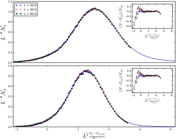
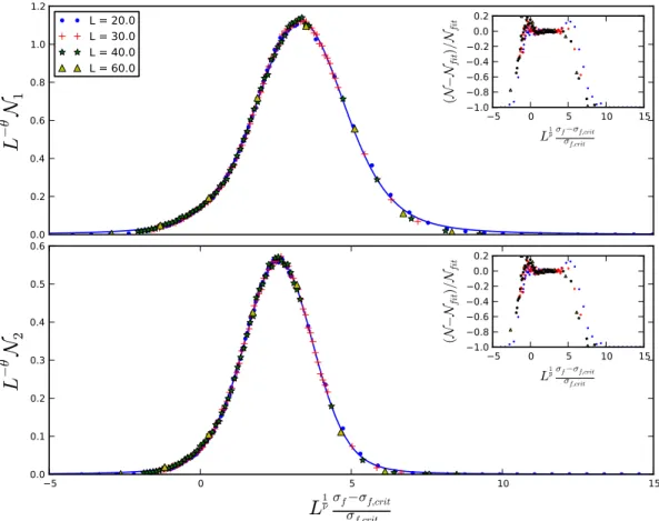
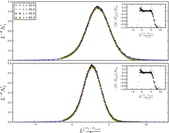
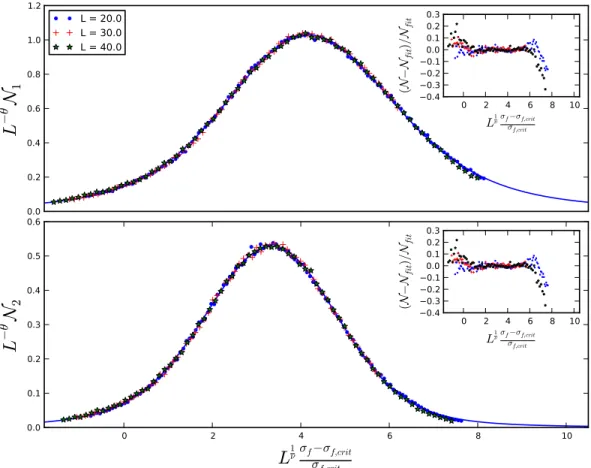
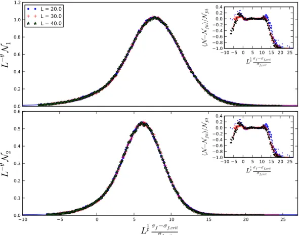
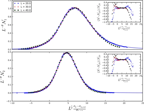
Section 3.5: Finite-Size Scaling of Spanning Avalanche Numbers
To determine the location and properties of the phase transition discussed in Section 2.2, either σb or σf is held constant and the other swept, and the numbers of spanning avalanches
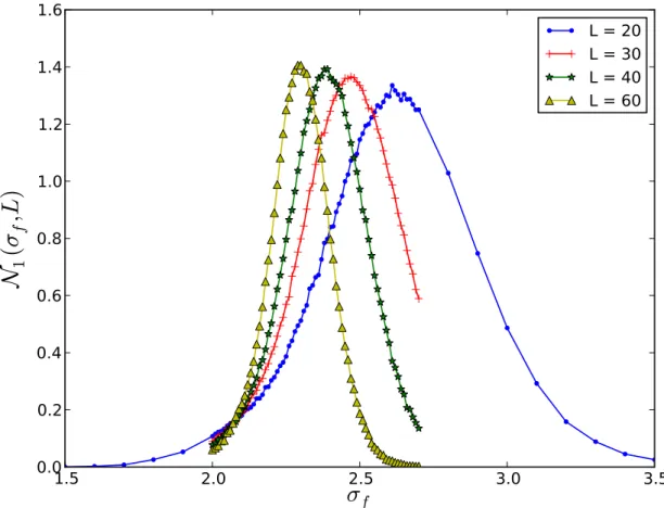
are found. Fig. 3.1 shows the results of one such sweep, in which σb is held constant and
σf is swept. The bumps in the numbers occur as the phase transition is crossed (at the
transition, avalanches of all sizes become important; cf. Section 2.2). As the plot shows, lattices with different sizes L produce different N vs. σf curves, and thus seem to indicate
1.5
2.0
2.5
3.0
3.5
σ
f
0.0
0.2
0.4
0.6
0.8
1.0
1.2
1.4
1.6
N
1
(
σ
f
,L
)
L = 20
L = 30
L = 40
L = 60
Figure 3.1: 1d Spanning Avalanche Numbers, for the case thatσb was held constant at 0.3
lattice.
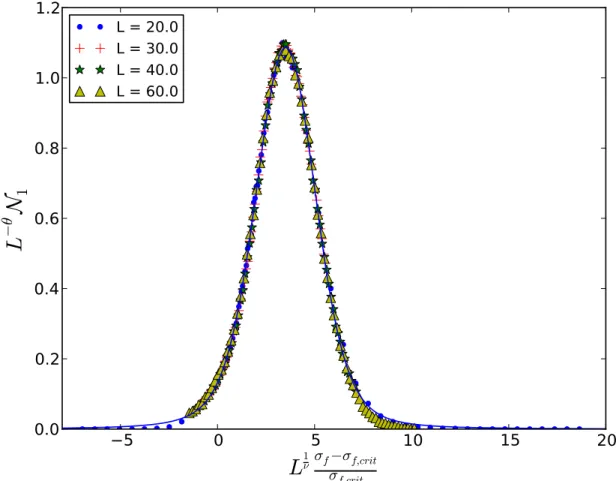
It is well-known that near such second-order transitions seemingly-different curves like these can often be made to collapse to the same curve by a careful combination of the variables (in the above case, these would beN1, σf, andL). In the context of size-dependent quantities,
this technique is known as finite-size scaling (Cardy, 1988; Goldenfeld, 1992;Cardy, 1996). Careful finite-size scaling analysis of the spanning avalanches in disordered Ising models was initiated in (P´erez-Reche and Vives,2003).
Consider a generic renormalization group fixed point for a finite-size system of size L. Under the standard RG length rescaling by a factor b (i.e. length → b−1length), a relevant variableuwith scaling exponent ν1 transforms asu→bν1u, where 1
ν >0 because uis relevant.
True critical behavior is only attained for an infinitely-large system, meaning the fixed point corresponds not only to u= 0 but also toL−1 = 0. Under the length rescaling, the inverse of the system size L−1 transforms as L−1 →bL−1, meaning that the inverse system sizeL−1 is a relevant variable with exponent 1.
This suggests that we should perform the usual critical-point scaling analysis, but adding L−1 as a new relevant variable. Above, we defined the scaling exponent of u as 1
ν. We now
define the scaling exponent of the spanning avalanche numbers Ni as θ. Now, perform an
RG length rescaling n times, in such a way that bnL−1 =l−01, where l−01 is a constant not too far away from the critical point (this is standard RG scaling analysis; cf. (Cardy,1996)). This gives
Ni(u, L) = bnθNi(bn/νu, bnL−1)
=LθN¯i(L1/νu),
(3.5)
where ¯Ni(x) =l0−θNi(xl
−1/ν
0 , l
−1
0 ) is the scaling function for the spanning avalanches. Now, if L−θNi is plotted against L1/νu, all the data should follow the same curve.
5
0
5
10
15
20
L
1ν
σ
f−σ
f,critσ
f,crit0.0
0.2
0.4
0.6
0.8
1.0
1.2
L
−
θ
N
1
L = 20.0
L = 30.0
L = 40.0
L = 60.0
Figure 3.2: Scaled 1d Spanning Avalanche Numbers, for constantσb = 0.3 and swept σf.
These are the same data as in Fig. 3.1, but with the scaling analysis explained in the text. This plot is also shown in Fig. 4.3.
comparing their values between different models (i.e. between different types of disorder) universality between these different models can be estimated.
As stated above, u is a scaling variable, a parameter that controls how far the system is from criticality, but how does it relate to the disorder parameter σ? A scaling variable should be dimensionless, and criticality should correspond to u= 0. Typically, such variables are identified with the physical parameters of the model; for example, the temperature T in a thermal phase transition corresponds to the scaling variable t= T−Tcritical
parameters. Since the pioneering work of (Perkovi´cet al., 1995), the usual definition of the scaling variable for avalanche studies of disordered Ising models has been
u0 = σ−σcritical
σ (3.6)
as opposed to the more traditional scaling variable definition
u= σ−σcritical σcritical
. (3.7)
However, a strong reason for using one over the other in these studies, beyond simply that some plots looked better with the former than with the latter, has not been made. Indeed, as Fig. 3.2 shows, the data obtained in the present work scale quite well using the traditional scaling variable u. While the scaling analysis shown here was repeated using the scaling variable u0, and this did provide reasonably-good scaling plots, the scaling analysis using u was uniformly superior to that using u0.
Thus, in this study, the traditional scaling variable u has been used exclusively. However, scaling collapses of 1d vs. 2d spanning avalanche numbers give equally strong scaling collapses yet different critical exponent estimates. This can be seen in the scaling plots shown in Section 4.1, where in each figure the 1d and 2d avalanche numbers have both been scaled. Considering that the choice of 1d vs 2d avalanches should be given preference in determining the critical exponents, both scalings were used to determine the final estimates of the critical parameters. Specifically, the final critical exponent values for a particular model (a particular model is defined by the pair of σb and σf values) reported in Section 4.3 were found by
averaging over the two values found from the two scaling collapses (1d and 2d avalanches), and the uncertainties are the standard deviations in these averages.
The scaling collapse of the data determines the location of the critical point (σf,critical or
σf,critical depending on the type of sweep performed), the correlation length critical exponent