IMPROVING METHODS FOR PROPENSITY SCORE ANALYSIS WITH MIS-MEASURED VARIABLES BY INCORPORATING BACKGROUND VARIABLES WITH
MODERATED NONLINEAR FACTOR ANALYSIS
Noah Greifer
A thesis submitted to the faculty at the University of North Carolina at Chapel Hill in partial fulfillment of the requirements for the degree of Master of Arts in the Department of Psychology
& Neuroscience (Quantitative) in the College of Arts & Sciences.
Chapel Hill 2018
ABSTRACT
Noah Greifer: Improving Methods for Propensity Score Analysis with Mis-Measured Variables by Incorporating Background Variables with Moderated Nonlinear Factor Analysis
(Under the direction of Patrick Curran)
TABLE OF CONTENTS
LIST OF TABLES ... vii
LIST OF FIGURES ... viii
LIST OF ABBREVIATIONS ... ix
INTRODUCTION ... 1
The Potential Outcomes Framework ... 2
Exchangeability and Confounding ... 3
Adjusting for Confounding ... 6
Balancing Scores and the Propensity Score ... 7
Estimating Propensity Scores ... 8
Estimating a Treatment Effect ... 10
Propensity Scores vs. Regression Models ... 11
Propensity Scores and Measurement Error ... 13
Factor Analysis and Factor Scores ... 16
Moderated Nonlinear Factor Analysis ... 18
Propensity Scores and MNLFA ... 21
CHAPTER 1: METHODS ... 23
Data Scenario ... 23
Latent and Observed Confounders... 24
Measurement Moderation ... 25
Treatment and Outcome Models ... 26
Impact. ... 27
DIF. ... 28
Number of Items. ... 29
Data Generation and Analysis ... 29
Effect Estimation Models ... 30
Method 1: Naïve Model. ... 30
Method 2: Individual Items. ... 31
Method 3: Simple FS. ... 31
Method 4: MNLFA Simple FS. ... 32
Method 5: Fully Inclusive FS. ... 32
Method 6: MNLFA Fully Inclusive FS. ... 33
Method 7: True LV. ... 33
Model Estimation ... 34
Criterion Variables ... 34
CHAPTER 2: RESULTS ... 38
Convergence and Aberrant Estimates ... 38
Score Quality ... 39
Factor Scores. ... 39
Propensity Scores. ... 39
Bias and Variability of Effect Estimates ... 40
Items. ... 40
Simple Factor Score. ... 41
MNLFA Simple Factor Score. ... 42
Fully Inclusive Factor Score. ... 43
True LV Values. ... 45
Covariate Balance ... 45
Balancing Performance. ... 46
Indicating Balance on the LV. ... 47
CHAPTER 3: DISCUSSION ... 49
Hypothesis 1: The presence of impact or DIF will yield biased effect estimates when using the standard estimators ... 50
Hypothesis 2: Incorporating MNLFA into standard estimators will yield improved estimates when impact or DIF are present... 52
Hypothesis 3: Using MNLFA when impact and DIF are not present will yield unbiased but imprecise results due to over-modeling ... 54
Simple vs. Fully Inclusive Methods... 55
Limitations ... 57
Recommendations ... 59
Future Directions ... 60
LIST OF TABLES
LIST OF FIGURES
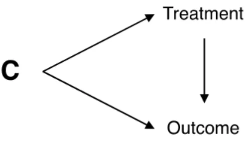
Figure 1. Nonparametric path diagram illustrating the basic structure of
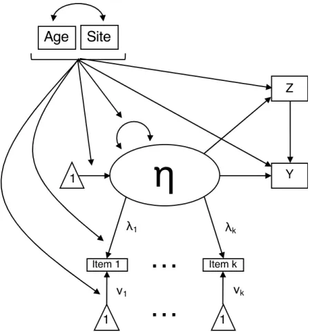
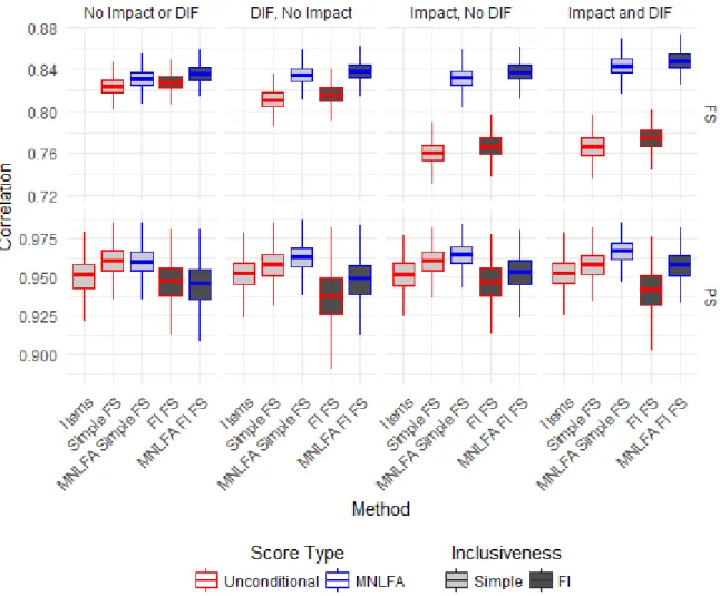
confounding. ... 62 Figure 2. Path diagram depicting the data-generating model. ... 63 Figure 3. Path diagrams corresponding to the four factor models fit. ... 64 Figure 4. Correlations between estimated factor scores and true values of the
latent variable (upper plot) and between estimated propensity scores and optimal
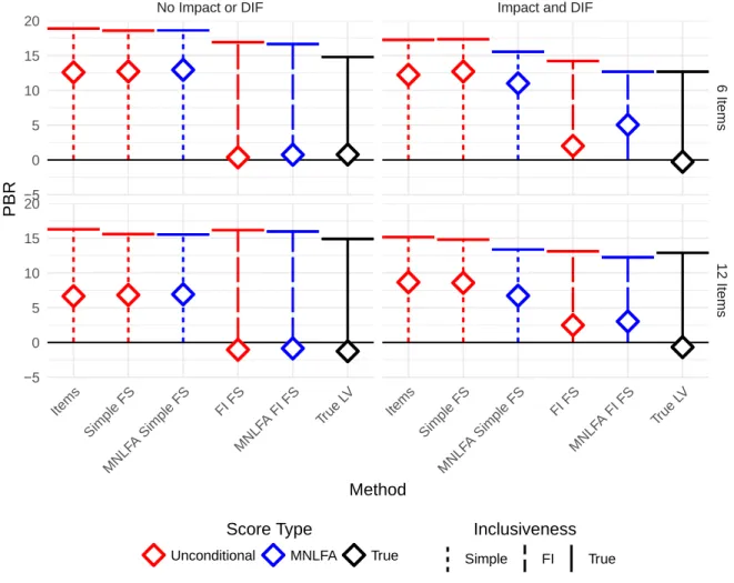
propensity scores (lower plot) for each method with six items. ... 65 Figure 5. Percent bias remaining (PBR) of each method in the “Impact absent,
LIST OF ABBREVIATIONS ATE average treatment effect
CBCL Child Behavior Checklist CE conditional exchangeability DIF differential item function IRT item response theory LV latent variable
MNLFA moderated nonlinear factor analysis PBR percent bias remaining
RMS root mean squared
RMSBD root mean squared balance discrepancy SMD standardized mean difference
SUTVA stable unit treatment value assumption wABC weighted area between curves
INTRODUCTION
Randomized control trials have long been considered the “gold standard” design method for making causal inferences in the social and health sciences (Jones & Podolsky, 2015). When randomization is successful, any observed difference in outcomes after receipt of the treatment can be due only to treatment status and not to some other variable that might otherwise explain the relationship between treatment status and outcome (Shadish, Cook, & Campbell, 2002). Although random assignment is frequently used in psychology to answer causal questions, often random assignment is unethical or impossible. For example, researchers cannot randomly assign whether people experience childhood trauma, use illicit substances in adolescence, or are held back a year in school, but clearly the causal effects of these events are of great concern to researchers and policymakers. There may also be scenarios in which random assignment is not desirable, because it involves forcing a subset of individuals into a treatment condition they might not otherwise want be placed in; the conclusions of randomized studies can therefore lack external validity (Rothwell, 2005).
convicted, which itself might explain why substance users have more convictions in adulthood. Instead of simple comparisons between conditions, researchers will have to rely on statistical methods and sets of assumptions to identify causal effects and make valid causal inferences for their data. These methods are further complicated by measurement error, ubiquitous in
psychology, in which the constructs of interest are often not directly observable.
The structure of this paper is as follows. First, I introduce the assumptions required and methods available for making causal inferences with social science data, with a focus on propensity score methods. Next, I describe the problems with propensity score methods caused by measurement error and recent attempts to solve these problems. Next, I present a new potential solution that builds off prior methods involving latent variable analysis by including a recent methodological innovation, namely moderated nonlinear factor analysis (Bauer, 2017; Bauer & Hussong, 2009). Finally, I present the results of a simulation study designed to examine the plausibility and effectiveness of this proposed method to improve the performance of
propensity score methods in conditions of measurement error; this is the focus of my work here. The Potential Outcomes Framework
The potential outcomes framework is a valuable conceptual and mathematical tool to understand the problems associated with making causal inferences. In this framework, each individual has two potential outcomes, Yz=0 and Yz=1, where Y is a continuous outcome variable and z is an instance of random variable Z denoting treatment status taking the values 0 (control) and 1 (treated). These correspond to the potential outcomes if the unit were to receive control and if the unit were to receive treatment. We can define the individual treatment effect for a unit i to be
𝜏𝑖 = 𝑌𝑖𝑧=1 – 𝑌
and the average treatment effect in the population (ATE) to be
𝐴𝑇𝐸 = 𝐸[𝑌𝑖𝑧=1 – 𝑌
𝑖𝑧=0] = 𝐸[𝑌𝑖𝑧=1] – 𝐸[𝑌𝑖𝑧=0] (2)
In fact, though, for each individual, only one of the potential outcomes is observed. The other is the counterfactual outcome (i.e., counter to fact). This is considered the fundamental problem of causal inference: neither E[Yiz=1] nor E[Yiz=0] can be directly computed to attain a causal effect estimate. Instead, we can compute functions only of the observed outcomes E[Yiz=1|Z=1] and E[Yiz=0|Z=0], the potential outcomes realized corresponding to the actual treatment
assignment of the individuals.
However, the expectations of the potential outcomes are identifiable under several assumptions. These are the stable unit treatment value assumption (SUTVA), positivity, consistency, and exchangeability (Foster, 2010). SUTVA requires that a unit’s potential outcomes do not depend on the treatment status of other individuals (and thus are “stable”). Positivity requires that it is theoretically possible for all units to be in either treatment condition (i.e., no combinations of qualities systematically exclude units from either condition).
Consistency requires that there are no unspecified versions of treatment. Although these
assumptions are worthy of study, the final assumption of exchangeability, described below, is the focus of this paper, and the aforementioned assumptions will be taken for granted here.
Exchangeability and Confounding
Exchangeability is a core assumption and requires that there is no association between treatment status and potential outcomes:
𝑌𝑧⊥ 𝑍 𝑓𝑜𝑟 𝑎𝑙𝑙 𝑧 (3)
assignment. The assumption of exchangeability will be the focus of this work and is the focus of most work in causal inference research. Conceptually, exchangeability can be thought of as the assumption that there are no alternative explanations for the observed association between actual treatment assignment and actual outcome value other than the causal effect of treatment on the outcome. In other words, there is no confounding.
Asymptotically, randomization guarantees exchangeability because when units are
randomized to conditions the joint distribution of factors that influence potential outcomes will be the same across conditions (even if the factors are not measured). In this way, treatment assignment is independent of potential outcomes (because it is independent of all covariates that relate to potential outcomes), and exchangeability is met. In this case,
𝐸[𝑌𝑧=1|𝑍 = 1] = 𝐸[𝑌𝑧=1] (4)
and
𝐸[𝑌𝑧=0|𝑍 = 0] = 𝐸[𝑌𝑧=0] (5)
Because the first expression in each of the equations (4) and (5) is identifiable from the observed data, the desired estimand—the unconditional expectation of each potential outcome—can be computed using equation (2). A simple comparison of group means will yield a valid estimate of the treatment effect.
Exchangeability can be extended to the case of conditionally randomized experiments, wherein within each level of some factor (i.e., a random variable C), randomization occurs and assignment is independent of potential outcomes. In this case, conditional on C, there is
𝑌𝑧 ⊥ 𝑍 |𝐶 = 𝑐 𝑓𝑜𝑟 𝑎𝑙𝑙 𝑧, 𝑐 (6)
For example, to examine the effect of a promising school policy intervention aimed at improving the academic performance of financially disadvantaged children, researchers might randomly assign schools in low income neighborhoods to treatment with 0.75 probability and might randomly assign schools in middle income neighborhoods to treatment with 0.5 probability. It is clear that neighborhood income class will affect the potential outcomes of the schools, regardless of treatment status, but conditional on (i.e., within) neighborhood class, treatment is independent of the potential outcomes, and so a marginal causal effect can be identified (Hernán & Robins, 2018). This insight is critical to understanding exchangeability in observational studies, which are more common than conditionally randomized experiments in psychology.
When randomization does not occur and, for example, individuals are allowed to choose their own treatment condition, equations (4) and (5) do not hold and the causal effect cannot be
immediately identified. Instead, a simple comparison of group means will include information both about the treatment effect and the other associations between assignment and potential outcomes. For example, if those with parents who have histories of conviction are more likely to engage in illicit substance use as adolescents, the difference in adult convictions between
adolescent substance users and abstainers will include not only the causal effect of drug use on the individual’s convictions but also the association between parental conviction history and the individual’s convictions through pathways other than the increased propensity to use substances. This failure to identify the correct causal effect is called “bias” and is a direct result of
adult convictions the outcome, and having parents with a history of convictions a common cause of treatment and outcome that creates confounding.
In observational studies, it may be possible to condition on a set of confounding variables and arrive at CE. This will be true if the observational study can be thought of as a conditionally randomized experiment: conditional on a set of pre-treatment variables, individuals are randomly assigned (with some nonzero probability) to condition (Hernán & Robins, 2018, Ch. 3).
Therefore, to identify causal effects in observational studies, one can condition on a set of pre-treatment variables associated with pre-treatment and potential outcomes and arrive at a valid
estimate of the causal effect without true randomization. The identification of the set of sufficient variables to eliminate confounding is its own area of research (e.g., Brookhart et al., 2006), but the focus for the rest of this study will be on the act of conditioning on those variables, given that they are already known.
Adjusting for Confounding
Three methods of conditioning on variables include matching, stratification, and regression. In matching, individuals in one treatment condition are matched to individuals in the other based on similarity of covariate values, and the causal effect estimate is the average of the pairwise outcome differences. In stratification, units are stratified into quantiles of covariate values, and treatment effects are estimated within each stratum. A problem with these two methods is that with many confounders, which are often necessary to eliminate confounding in observational studies, these methods fail: it will be impossible to find units with the same or even similar values of the entire set of covariates, yielding units without matches and strata with too few units (Rosenbaum & Rubin, 1984). This problem is often known as the “curse of dimensionality.”
commonly used as a statistical method to condition on sets of variables in conditionally randomized and observational studies. A weakness of regression is that the functional form of the relationship between all of the included covariates and the outcome must be correctly specified in the regression model, or else residual confounding can occur (Schafer & Kang, 2008). For example, if the true outcome model includes interactions and nonlinear terms but a simple linear regression missing those forms is specified, the effect estimate will be biased and inconsistent (Hernán & Robins, 2018, Ch. 15; Schafer & Kang, 2008). There are other reasons why researchers may want to avoid regression in favor of some other method to adjust for
confounding; these will be discussed later to contrast regression with the methods presented next. Balancing Scores and the Propensity Score
Consider a set of variables C for which conditioning on C is sufficient to eliminate confounding and arrive at CE. A balancing score b(C) is a value or set of values that, when conditioned upon, yields conditional independence between the covariates and the treatment, thereby satisfying the requirements for CE. The full set of confounding variables itself is (trivially) a balancing score. However, as described above, conditioning on the full set through matching or stratification can fail due to the curse of dimensionality, and conditioning on the full set through regression requires model assumptions that are unlikely to be met. In their landmark paper, Rosenbaum and Rubin (1983) discovered a unidimensional balancing score, known as the propensity score, which could allow for matching and stratification to achieve exchangeability. Formally, they discovered a b(C) such that
𝑌𝑧 ⊥ 𝑍 |𝑪 ⇒ 𝑌𝑧 ⊥ 𝑍 |𝑏(𝑪), (7)
where
𝑏(𝑪) ≡ 𝑃(𝑍 = 1|𝑪). (8)
confounding and arrive at CE, then conditioning on the conditional probability of receiving treatment given C—the propensity score—is also sufficient to arrive at CE. In a conditionally randomized experiment, the probability of receiving treatment is set by the researcher, and non-parametric techniques like matching and stratification on this known probability will yield unbiased estimates of a treatment effect.
A variety of methods have been developed for matching on the propensity score, including the traditional and simple nearest neighbor matching, as well as more sophisticated alternatives such as full matching (Stuart & Green, 2008) and genetic matching (Diamond & Sekhon, 2013). With stratification, researchers typically form quantiles of the propensity score and estimate treatment effects within each quantile; this technique is used less frequently than matching (Thoemmes & Kim, 2011). Propensity scores can be used in inverse probability weighting for marginal structural models (Robins, Hernan & Brumback, 2000), where a function of the propensity score is used as a sampling weight in weighted estimation. Occasionally, the
propensity score itself is used as a covariate in a regression model, but this method has fallen out of favor due to its poor empirical properties and additional required assumptions (Austin, 2011; Thoemmes & Kim, 2011). The primary focus here will be on propensity score weighting. Estimating Propensity Scores
interactions, and other non-linear terms; machine learning techniques such as generalized boosted modeling (McCaffrey, Ridgeway, & Morral, 2004) can simplify this process by
requiring fewer modeling decisions from the user in cases of uncertainty (Lee, Lessler, & Stuart, 2010).
The resulting estimated propensity scores must then be evaluated for their ability to achieve CE by empirically examining whether, after conditioning on the propensity score, the joint distributions of covariates are similar across treatment groups (Stuart, 2010). This distributional similarity, an approximation of CE in the sample, is often referred to as balance. Balance
assessment is an ongoing area of research, but typical methods involve comparing the means and higher moments of covariate distributions and interactions across treatment groups and using visual diagnostics such as kernel density and Q-Q plots (Kainz et al., 2017). A common and recommended measure of balance is the standardized mean difference (SMD), defined by the following expression (Austin, 2011):
𝑆𝑀𝐷 = 𝑀1− 𝑀0 √𝑠12+ 𝑠02
2
(9)
where M1 and M0 are the (weighted) group means of the covariate under study, and s12 and s02 are the group variances. In propensity score weighting, the SMD is computed with the group means weighted by the estimated propensity score weights, but the group variances remain unweighted (Stuart, 2010). Typically, SMD values below 0.10 in absolute value are considered adequate (Stuart, 2010). It is important to note that propensity score models are not to be
evaluated on traditional model evaluation criteria such as goodness of fit or parsimony; attaining balance on the covariates of interest is paramount (Stuart, 2010).
balance, the propensity score model can be respecified, such as by adding squared terms or interactions, and reevaluated until balance is achieved (Rosenbaum and Rubin, 1984; Stuart & Rubin, 2008; Stuart, 2010). Because this process does not involve the outcome variable, there is no risk of capitalizing on chance to arrive at a specific treatment effect estimate; the propensity score stage of a full analysis is akin to the design stage of a study, in that applying the propensity score is essentially adjusting the selection parameters for the sample (Rubin, 2001). Unlike typical statistical analyses, overfitting to the data is not a problem because the goal of propensity score analysis is to arrive at sample covariate balance irrespective of the interpretability,
plausibility, reproducibility, or parsimony of the propensity score model (Augurzky & Schmidt, 2001; Stuart, 2010).
Estimating a Treatment Effect
Once propensity scores have been estimated and balance has been achieved, an analyst can then estimate the treatment effect in their propensity score-conditioned data. For propensity score matched samples, a matched pairs t-test on the matched samples is recommended (Austin, 2011). For propensity score weighted data, an outcome regression model can be specified as follows:
𝐸[𝑌𝑗] = 0+1𝑍𝑗, (10)
Propensity Scores vs. Regression Models
In psychology, the practice of statistically modeling relationships among variables using regression or structural equation modeling is popular (Foster, 2010). Researchers can specify a parametric model for the outcome conditional on a linear combination of predictors, including treatment and variables required to eliminate confounding. The estimated treatment effect can then often be identified by examining the coefficient estimate for the treatment variable in the model (Schafer & Kang, 2008). On the other hand, propensity score methods are explicitly a non-modeling approach, in that the functional form of the relationship between the covariates and the outcome variable does not have to be modeled (Ho, Imai, King, & Stuart, 2007). Though the propensity score itself must be modeled, the process and reasons for modeling the propensity score vastly differ from those of confirmatory parametric models, opening up the possibility of employing machine learning and other optimization-based techniques that would normally be reserved for exploratory data analysis.
is done without considering the outcome data or a treatment effect estimate, propensity score methods do not face these issues.
Despite these potential pitfalls, regression can be a valuable tool for causal inference. It has been shown that when researchers apply regression and propensity score methods separately to analyze the same data, the substantive conclusions are almost identical (Shah, Laupacis, Hux, & Austin, 2005). Several authors recommend regression on datasets preprocessed through
propensity score or other matching methods (e.g., Ho, Imai, King, & Stuart, 2007; Rubin, 2001). Freedman and Berk (2008) found in their simulations that regression alone actually performed better than using propensity score weights alone or propensity score weighted regression. Indeed, there is still debate about the value of propensity score methods when linear regression often arrives at the same conclusion and does so with greater apparent precision (Shadish, Clark, & Steiner, 2008).
In the end, the debate boils down to a bias-variance tradeoff: with propensity score methods, there is a major emphasis on reducing bias, often at the expense of statistical efficiency (i.e., by removing cases after matching or down-weighting cases with weighting); whereas with
Propensity Scores and Measurement Error
In many of the social sciences, psychological variables can produce confounding because they are often related both to treatment selection (such as when individuals get to choose their own treatment) and to outcomes (such as when the outcome depends on motivation or is caused by baseline psychological characteristics). A major issue with psychological variables is that they are almost always measured with error (Bollen, 2002). Until recently, the problems associated with conditioning on an indicator of a mis-measured variable rather than on the true variable itself had been largely ignored in the causal inference literature. Steiner, Cook, and Shadish (2011) were the first to systematically investigate the effects of measurement error in covariates of the propensity score model on bias in the estimated treatment effect. They found that decreasing the reliability of measures of latent covariates associated with the treatment and outcome led to increased bias in treatment effect estimates. Other researchers found similar results in simulations that attempted to provide solutions to the problem of measurement error (e.g., Jakubowski, 2015, McCaffrey, Lockwood, & Setoji, 2013). Rodríguez De Gil et al. (2015) ran a large, comprehensive simulation study examining the effects of covariate unreliability on treatment effects estimated with propensity scores. They found that even small unreliability in covariates (e.g., reliabilities of .8) can lead to marked increases in bias, increased Type I error rates, and decreased confidence interval coverage. They did not examine a solution to these problems.
subclassification on latent classes (Masyn & Walderman, 2016). Although promising, most current approaches have limitations that hamper their widespread use: they are challenging to implement for substantively oriented researchers, some require external validation samples or otherwise untestable but major distributional assumptions, and they are still in their infancy, with little empirical validation.
Another solution that has gained some attention is to use latent variable (LV) models to generate estimates of the mis-measured covariate and then use those estimates in place of the true variable in standard propensity score analysis. This method involves generating factor scores from the observed indicators of the LV using standard factor analysis or principal components analysis. Raykov (2012) proposed this solution and supported it with analytical derivations and a simulated demonstration of its efficacy. Jakubowski (2015) explored this method as well, using simulations to more systematically examine its effectiveness under a variety of circumstances, including treatment model misspecification. Both authors found modest reductions in bias relative to using the observed covariates in propensity score analysis.
precedent for including the outcome in estimating the predictor of that outcome.
First, the Mantel-Haenszel technique, used to determine whether a test item functions differentially for two groups of units that are otherwise identical on their level of the measured construct, involves matching units with similar levels of the construct to be measured and comparing their responses to items (Michaelides, 2008). Holland and Thayer (1988) and Zwick (1990) found that matching on a proxy for the construct that included the item under study (i.e., the item for which the differential functioning between groups was in question) yielded superior performance for accurately assessing whether the item functioned differentially. In this way, the relationship between group membership and item response is examined conditional on a measure that includes the item response, similar to how Nguyen et al. (under review) proposed that the outcome of the propensity score model (i.e., the treatment) should be used to construct the score that is used as a predictor of that same outcome.
distal outcome is included as a covariate in the latent class model used for class assignment before the outcome is regressed on class membership (Bray, Laza, & Tan, 2015).
Instead, Burt (1976) described the procedure of using outcomes as indicators of LV models as leading to “interpretational confounding,” in that the meaning of the LV (and therefore its relationship with its indicators) changes when including an outcome in its measurement model. To the degree the meaning of the LV affects its relationship with an outcome, some authors argue that measures should be taken to separate the measurement step and outcome modeling step entirely (Burt, 1976). The approach of Nguyen et al. (under review) explicitly violates this recommendation by including the outcome (i.e., the treatment) in the measurement model and using the estimated scores from that model in predicting the same outcome.
There is both theoretical precedent and controversy in the use of the treatment as an indicator to estimate factor scores for propensity score analysis. Below I discuss factor scores and
measurement models in more detail, primarily considering standard measurement models (in the sense that only indicators of a LV, as opposed to outcomes, are included).
Factor Analysis and Factor Scores
Factor scores, also known as scale scores in item response theory (IRT), are point estimates of units’ values on a LV given some indicators and a model linking the LV to the indicators (i.e., the measurement model). There are variety of ways to compute factor scores (Grice, 2001), though they are often highly correlated with each other (Fava & Velicer, 1992). The first step is often to specify and estimate a (generalized) factor score model, which parametrically links the LV to its indicators, using an equation such as
µ𝑖𝑗 = 𝑔𝑖−1(𝜈
𝑖 + 𝜆𝑖𝜂𝑗) (11)
assumed be normally distributed as
𝜂𝑗 ~ 𝑁(𝛼, 𝜓) (12)
where α and ψ are the mean and variance, respectively, of the LV, and νi and λi are parameters describing the linear relationship between ηj and µij (Bauer, 2017; Bauer & Hussong, 2009). In relation to a generalized linear model, gi-1(.) is an inverse link function, which may differ for each item depending on its type; a response function is also specified to relate the expected value of the indicator µij to actual indicator values uij. For example, a linear factor model with
continuous indicators might include an identity link (and inverse link) and a normally distributed response function, while a 2-PL IRT model with binary indicators would include a logit link and a binomial response function (Bauer & Hussong, 2009). For this 2-PL model, the relationship between µij and the observed response uij for item i would be defined as P(uij = 1| ηj) = µij.
Once parameters for the factor model have been estimated, they can be used to generate factor scores based on individuals’ patterns of responses and assumptions about the distribution of the LV. For each individual, a “posterior” distribution f for the LV can be formed by taking the product of the conditional item response functions (i.e., measurement equations) for each item and the conditional LV distribution (usually specified as Gaussian), as in the following equation:
𝑓(𝜂𝑗|𝒖𝑗) = ∏ 𝑇𝑖(𝑢𝑖𝑗|𝜂𝑗)𝜙(𝜂) 𝑛𝑖𝑡𝑒𝑚𝑠
𝑖=1
(13)
continuous items (Grice, 2001), Lu and Thomas (2008), building off core results of Skrondal and Laake (2001), recommend using the expected a posteriori (EAP) score estimates, which involve computing the expectation of this posterior distribution, when the scores are to be used as predictors in regression models.
A problem with estimating factor scores, and with factor analysis in general, is factor indeterminacy; perfect estimates of the LVs are impossible because the LV does not have a posterior point distribution after observing and modeling the indicators (Maraun, 1996). That is,
𝑓(𝜂𝑗|𝒖𝑗) has nonzero variance. Modeling more information about the LV can reduce
indeterminacy by reducing the posterior variance, yielding more precise estimates of the LV in the form of factors scores (Fava & Velicer, 1992). This information can come in the form of a larger sample size, more indicators, and higher multiple correlation of other covariates with the LV (Bollen, 2002). Given a constant sample size, including more indicators (i.e., consequences) of the LV and modelling covariances with other observed variables will thereby reduce factor indeterminacy, leading to superior factor score estimates (Mislevy et al., 1992). These properties may help explain why the approach to propensity score estimation of Nguyen et al. (under review) led to improved performance of the propensity scores: including the treatment variable as a consequent of the LV increased the number of its indicators, and including the covariances between other covariates and the LV increased the multiple correlation for the LV, both of which reduce its indeterminacy by reducing the variance of it posterior distribution.
Moderated Nonlinear Factor Analysis
same scoring algorithm exists for all units, estimates of the LV are biased and imprecise, resulting from incorrect modeling of the relationship between the LV and its indicators. Two ways background variables might influence measurement are known as impact and differential item function (DIF). Impact occurs when background variables affect the distribution of the LV
(i.e., by creating different values of α and ψ in equation (12) for each individual). The LV mean and variance for individual j are instead specified as
𝛼𝑗 = 𝑓𝛼(𝑿𝑗) (14)
and
𝜓𝑗 = 𝑓𝜓(𝑿𝑗), (15)
where αj and ψj are the mean and variance, respectively, of the LV for individual j with background variables Xj, and fα and fψ relate Xj to αj and ψj. DIF occurs when background variables affect the parameters relating the LV to its indicators (i.e., by creating different values of νi and λi in equation (11) for each individual). In this case, the item intercept and loading for individual j are specified as
𝜈𝑖𝑗 = 𝑓𝜈𝑖(𝑿𝑗) (16)
and
𝜆𝑖𝑗 = 𝑓𝜆𝑖(𝑿𝑗), (17)
where νij and λij are the factor intercept and loading for item i for individual j with background variables Xj, and fνi and fλi relate Xj to νij and λij.
moderated nonlinear factor analysis (MNLFA), an expansion of generalized factor analysis that allows for the simultaneous modeling of the relationships between covariates and both the LV and its indicators (Bauer & Hussong, 2009; Curran, et al., 2014). Doing so involves specifying a model for the LV mean, a model for the LV variance, and models for the parameters in the measurement models of the indicators, all of which can contain background covariates of any variable type, subject to identifiability constraints. Thus, each of the parameters estimated in the models in equations (11) and (12) can vary across individuals, and can be modeled in terms of functions containing background covariates as in equations (14) through (17).
The models are simultaneously estimated, yielding parameter estimates that can be used to generate factor score estimates using an updated version of equation (13) (Bauer & Hussong, 2009):
𝑓(𝜂̂𝑗|𝒖𝑗, 𝑿𝑗) = ∏ 𝑇𝑖(𝑢𝑖𝑗|𝜂𝑗, 𝑿𝑗)𝜙(𝜂𝑗|𝑿𝑗) 𝑛𝑖𝑡𝑒𝑚𝑠
𝑖=1
(18)
which now conditions on Xj. Ti and ϕ now explicitly involve j and involve estimating the parameters in fα, fψ, fνi, and fλi.
Curran, et al. (2016) used a simulation to examine the performance of this technique and others for estimating factor scores in various conditions of covariate involvement in the measurement model. Simulation factors included percent of items with DIF, ratio of mean impact to variance impact, number of items, and the magnitude of DIF. Examined scoring models included proportion scores (i.e., the mean of the indicators), unconditional MNLFA (i.e., a 2-PL IRT model), MNLFA accounting for impact, and MNLFA accounting for both impact and DIF. The authors found fairly substantial improvements in factor score recovery (as
the estimated scores) under all scenarios when using MNLFA that accounted for both impact and DIF, even when the covariate involvement was small, and especially when it was large. The authors conclude by recommending the inclusion of background variables when available through MNLFA in estimating factor scores.
Propensity Scores and MNLFA
Given these findings, it would appear that involving background variables in factor score estimation for propensity score modeling is a plausible solution to the problem of improving propensity score-based methods with mis-measured covariates. In settings in which propensity scores are commonly used, background variables are often plentiful, as they are included in the models used to estimate the propensity scores. These background variables may be able to provide more information than solely their prediction of the probability of treatment assignment; including some of them in a MNLFA model for the estimation of the factors scores of the latent confounder may also help to decrease bias and improve the precision of the effect estimate. As the use of factor scores in propensity score estimation is still in its infancy, these possibilities have not yet been examined, and they may provide a benefit to research assessing causal effects in the ubiquitous circumstance of confounding and measurement error.
on these causal methods often used in other disciplines with little development in accounting for measurement error.
Drawing from theory and prior results on measurement error, factor scoring, and propensity score analysis described previously, I proposed the following hypotheses to be addressed in this study. First, I hypothesized that failing to model impact and DIF when they are present will yield degraded factor score estimates, thereby biasing causal effect estimates in addition to increasing their variability. Second, I hypothesized that using MNLFA and including background covariates will improve causal effect estimation by yielding factor score estimates that better emulate the true confounder addressed using propensity scores, thereby reducing the bias and variability of the effect estimate. Third, I hypothesized that in cases of uncertainty about the population impact and DIF effects, the detriments of over-modeling when impact and DIF are not present will be outweighed by the benefits of correct modeling when they are present, especially when more information about the LV is available. Finally, I hypothesized that the factor scores generated from models that most closely matched the data-generating model would yield the most accurate information about balance on the true latent confounding variable.
CHAPTER 1: METHODS Data Scenario
To provide concreteness to the simulation, it is helpful to consider a hypothetical
observational study comparing the effect of a standard vs. an experimental after-school program for elementary school students on emotional wellbeing at the program’s end. We might imagine this study spread over two sites implementing the same programs. Students are allowed to choose the program in which they take part, and we can imagine their choice depends on factors including site-specific characteristics, their age, and their level of an LV (e.g., depression) as measured by an error-prone psychological scale with binary items and known DIF such as the Child Behavior Checklist (CBCL; Achenbach & Edelbrock, 1981). In this example, our “treatment” is the experimental program, while the “control” is the standard program. The
outcome is measured emotional well-being at the program’s end, which itself is known to depend on a variety of factors, including those that influence selection into the chosen program1. We will imagine that age, site, and the LV constitute a sufficient set of variables to identify the causal effect of the experimental program relative to the standard one. We can assume one is interested in the ATE, the hypothetical average effect of moving all students from the standard program to the experimental program. We will imagine that levels and the measurement of the LV may be affected by each student’s site and age, which is plausible given prior research (e.g., Curran et al., 2014).
1 For the purposes of this simulation, it will be assumed that the outcome construct of interest is measured perfectly;
I simulated data consistent with the path model in Figure 2. The data-generating model includes two components: a binary treatment (program) with a causal effect on an observed continuous outcome (well-being) confounded by an observed binary variable (site), an observed continuous variable (age), and a latent continuous variable (depression); and a measurement model for the LV that includes binary indicators, mean and variance impact from the observed confounders, and slope and intercept DIF from the observed confounders. The causal portion of the model is a setup common in propensity score simulations (e.g., Jakubowski, 2015; Nguyen et al., under review), while the measurement portion is similar to that used in Curran et al. (2016). Latent and Observed Confounders
The LV is measured with a set of k binary items. I specified the corresponding measurement model as follows2: for j = 1, …, n individuals assessed on i = 1, …, k binary indicators, each indicator wij will follow a Bernoulli distribution with probability pij defined by the factor model as
𝑝𝑖𝑗 = (1 + 𝑒𝑥𝑝(−(𝜈𝑖𝑗 + 𝜆𝑖𝑗𝜂𝑗)))−1 (M1)
where νij is the intercept of item i for person j, λij is the loading of item i for person j, and ηj is value of the LV for person j, distributed as 𝜂𝑗 ~ 𝑁(𝛼𝑗, 𝜓𝑗). This corresponds to a generalized linear model with a logit link and a Bernoulli response function, equivalent to a 2-PL IRT model when considering ηj as latent.
The observed covariates site and age were generated, respectively, as being drawn from a Bernoulli distribution with probability 0.6 and from a uniform distribution with bounds (-3, 3) (i.e., as if age were centered at its population mean for the group of interest). Although typically many more confounders and at least several moderators of the factor model would be present in
an analysis with real data, here I limited my simulation to just two variables for simplicity of illustration, with the hope that results would generalize to situations with more variables and variables of types other than binary and uniform continuous. Substantive theory would typically drive the selection of these variables.
Measurement Moderation
I defined measurement moderation using the following models: I defined mean and variance impact, respectively, as
𝛼𝑗 = 𝛾0 + 𝛾1𝑎𝑔𝑒𝑗+ 𝛾2𝑠𝑖𝑡𝑒𝑗+ 𝛾3𝑎𝑔𝑒𝑗 × 𝑠𝑖𝑡𝑒𝑗 (M2) and
𝜓𝑗 = 𝛽0𝑒𝑥𝑝(𝛽1𝑎𝑔𝑒𝑗 + 𝛽2𝑠𝑖𝑡𝑒𝑗). (M3)
These equations are instantiations of equations (14) and (15). By this specification, the mean (αj) and variance (ψj) of the LV depend on (i.e., are impacted by) the levels of age and site; there is also an interactive effect of age and site on the mean (i.e., the effect of age on the LV mean is moderated by site). Equation (M3) for the LV variance ψj corresponds to a log-linear model so that the variance is bounded at 0 (Bauer, 2017; Bauer & Hussong, 2009). The parameters were chosen so that the marginal LV mean and variance were 0 and 1, respectively, in the population.
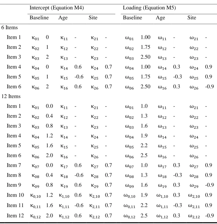
I defined intercept and loading (i.e., slope) DIF, respectively, as
𝜈𝑖𝑗 = 𝜅0𝑖+ 𝜅1𝑖𝑎𝑔𝑒𝑗 + 𝜅2𝑖𝑠𝑖𝑡𝑒𝑗 (M4) and
𝜆𝑖𝑗 = 𝜔0𝑖+ 𝜔1𝑖𝑎𝑔𝑒𝑗 + 𝜔2𝑖𝑠𝑖𝑡𝑒𝑗 (M5)
Treatment and Outcome Models
I specified the treatment effect model as follows, consistent with many propensity score simulations, notably Nguyen et al. (under review). I defined the treatment selection model as
log ( 𝑒𝑗
1 − 𝑒𝑗) = 𝑎0+ 𝑎1𝑎𝑔𝑒𝑗 + 𝑎2𝑠𝑖𝑡𝑒𝑗 + 𝑎3𝜂𝑗 (M6)
where ej is the probability of selecting the experimental program; that is, ej is the “true” propensity score (i.e., the model-generated probability of treatment assignment for each
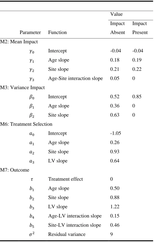
individual). This model is consistent with a logistic regression model where selection probability is determined only by site, age, and the LV. Program selection (Zj) is drawn from a Bernoulli distribution with probability ej for each unit j. The coefficients are listed in Table 1 and were chosen so that age, site, and the LV uniquely explain 5%, 5%, and 10%, respectively, of the variance in the logit of the true propensity scores, and the marginal probability of treatment is .35. These reflect small to medium effect sizes for the observed covariates and a medium effect size for the LV (Cohen, 1988, p. 413). SMDs (defined in equation 9) were 0.52 (age), 0.39 (site), and 0.80 (LV); these indicate significant covariate imbalance, especially for the LV, given that absolute SMDs of 0.10 or lower are considered tolerable (Stuart, 2010).
I defined the outcome model as
𝑌𝑗 = 𝜏𝑍𝑗+ 𝑏1𝑎𝑔𝑒𝑗+ 𝑏2𝑠𝑖𝑡𝑒𝑗+ 𝑏3𝜂𝑗 + 𝑏4𝑎𝑔𝑒𝑗 × 𝜂𝑗+ 𝑏5𝑠𝑖𝑡𝑒𝑗 × 𝜂𝑗
+ 𝜀𝑗
(M7)
differ only on Zj. Thus, τ is the causal effect of the experimental program on the outcome, and its estimate is the causal effect estimate that is the focus of the analysis of the simulations. The coefficients are listed in Table 1 and were chosen so that age and site each uniquely explained 6% of the variance in the outcome, the LV uniquely explained 12% of the variance in the
outcome, and the interactions each uniquely explained 2% of the variance in the outcome, so that all variables jointly explained 34% of the variance in the outcome. Together with the treatment selection, these parameters created significant confounding by the covariates, yielding an unadjusted treatment effect estimate with a Cohen’s d of approximately 0.6, indicating a
moderate to large effect of treatment (Cohen, 1988, p. 40), when the true treatment effect was 0. The residual variance (σ2) was chosen to scale and identify the effects of the covariates.
Design Factors
The design factors include the presence of impact (two levels), the presence of DIF (two levels), and the number of items (two levels), for a total of eight cells. Each cell was replicated 1000 times, for a total of 2 x 2 x 2 x 1000 = 8000 simulated data sets. Each data set contained 1000 individuals, which is reasonable for a two-site observational study and appropriate for both MNLFA and propensity score applications (e.g., Curran et al., 2017; Nguyen, Ebnesajjad, Stuart, Kennedy, & Johnson, 2018). Sample size will not be included as a varying design factor, given that its effects are predictable and Curran et al. (2016) found meager effects and no interactions with other design factors.
the LV and site of .21, which correspond to medium correlations commonly observed in practice (coefficient values are in Table 1). In the “impact absent” condition, the LV mean model
contained only the linear terms, and the LV variance was constant across individuals. In the “impact present” condition, an interaction between site and age was included in the LV mean model, and covariate effects were also included in the LV variance model (M3) so that the variance of the LV differed for each individual based on their covariate values. The coefficients of the variance model are listed in Table 1 and were chosen so that across individuals, the inter-quartile range of the model-generated LV variances was 0.5, corresponding to a medium amount of variability in the variances due to age and site, which was enough to perturb estimates using traditional method methods in Curran et al. (2016) and differentiated the results between the “impact present” and “impact absent” conditions in pilot testing. To ensure equality across conditions, parameters were chosen so that the marginal mean and variance of the LV were approximately 0 and 1, respectively, in the population.
DIF. I defined the presence of DIF as covariate effects on the intercept and loading
endorsements ranged between .5 and .75. Item communalities, computed as the squared correlation between the LV and the continuous latent propensity underlying the item
endorsement probabilities (Long, 1997), ranged from .23 to .7. The parameters and proportion of items with DIF are comparable to those found in empirical integrative data analysis applications, including Curran et al. (2014), and differentiated the results between the “DIF present” and “DIF absent” conditions in pilot testing. Specific values are in Table 2.
Number of Items. The number of items was either six or 12. As in many simulation studies,
the effect of the number of items is straightforward: the more items, the better the precision of the estimates because of increased factor determinacy (Bollen, 2002). This was found in both Curran et al. (2016) and Jakubowksi (2015). The reason for including it here was to examine whether the potential loss in precision due to over-modeling impact and DIF when there are none is comparable to the gain in efficiency when increasing the number of items. Curran et al. (2016) also found in metamodels that the number of items interacted with other design factors, including the magnitude of impact and DIF, which are studied here.
Data Generation and Analysis
Effect Estimation Models
Within each simulation, several estimation models were employed. In all but the naïve model (defined below), the following steps occurred. First, a score was estimated to represent the LV. Second, a logistic regression model was fit with treatment status as the response and the
observed covariates and the estimated LV score as predictors; this served as the propensity score model from which predicted probabilities were estimated as propensity scores. Third, the
propensity scores were transformed into weights with the following formula:
𝑤𝑗 = 𝑍𝑗 𝑒̂𝑗 +
1 − 𝑍𝑗
1 − 𝑒̂𝑗, (M8)
where 𝑍𝑗 is the treatment status for individual j and 𝑒̂𝑗 is their estimated propensity score. These weights are appropriate for estimating the ATE (Austin, 2011). Finally, an outcome regression model as specified in equation (10) was fit using the estimated weights for WLS estimation to acquire a treatment effect estimate for each data set. Additionally, using each set of weights, I computed the weighted SMD of the estimated LV score between the treated and control groups, and the same for the true value of the corresponding LV; these served as balance summaries for the estimated and true LVs.
The following are the methods that were employed in this simulation, which involve the basic, current best practice, and proposed improved methods.
Method 2: Individual Items. In this method, no LV scores were estimated; the propensity score model was fit using the individual items and the observed covariates to predict the log odds of treatment, as follows:
log ( 𝑃(𝑍𝑗 = 1) 1 − 𝑃(𝑍𝑗 = 1)
) = 𝑏0+ 𝑏1𝑎𝑔𝑒𝑗+ 𝑏2𝑠𝑖𝑡𝑒𝑗 + ∑ 𝑏𝑖+2𝑋𝑖𝑗 𝑘
𝑖=1
(M9)
where 𝑋1𝑗, … , 𝑋𝑘𝑗 are the k indicators for the LV. This approach was examined by Jakubowski (2015), Nguyen et al. (under review), and Raykov (2012) and represents an approach
recommended by Steiner, Cook, and Shadish (2011) to improve propensity score estimation with potentially unreliable variables. This technique might be typically employed when several
observed variables seem to measure the same construct but may not clearly fall within a known factor structure. To compute the balance summary for this method, I computed the weighted SMD for each item between the treated and control groups and then used the mean of these SMDs to serve as the balance measure.
Method 3: Simple FS. In this method, an unconditional generalized factor model (i.e., a
2-PL IRT model, not including the observed covariates) was fit to generate the factor scores. Figure 3A depicts a path diagram corresponding to the fitted model. The estimated factor scores
𝜂̂ were computed using EAPs and were used in the following logistic regression model:
log ( 𝑃(𝑍 = 1)
1 − 𝑃(𝑍 = 1)) = 𝑏0+ 𝑏1𝑎𝑔𝑒𝑗+ 𝑏2𝑠𝑖𝑡𝑒𝑗+ 𝑏3𝜂̂𝑗 (M10)
mean and variance were fixed at 0 and 1, respectively, and all intercepts and loadings were freely estimated.
Method 4: MNLFA Simple FS. I fit a conditional (i.e., MNLFA) generalized factor model to the items, modeling mean impact on the LV from site, age, and their interaction; variance impact on the LV from age and site modeled with a log-linear function (Bauer & Hussong, 2009); and intercept and loading DIF from age and site on half of the items. Figure 3B depicts a path diagram corresponding to the fitted model. When DIF and impact were present, this
MNLFA model corresponded to the data-generating model for the LV and items; otherwise, this model involved over-modeling nonexistent impact or DIF. DIF was modeled for the “correct” indicators, i.e., those indicators that in the “DIF present” condition had DIF (and therefore over-modeling non-existent DIF for those same items in the “DIF absent” condition). To identify the model, the mean and variance at the reference levels of the covariates (i.e., at 0) were fixed at 0 and 1, respectively, and all loadings were freely estimated. Factor scores 𝜂̂ were estimated from this model using EAPs of the conditional LV distribution and measurement functions as in Curran et al. (2016) and used to estimate propensity scores from the logistic regression model in equation (M10) and to compute the balance summary.
Method 5: Fully Inclusive FS. I fit a structural equation model linking the covariates and
the LV to the treatment (including the items as indicators), and then generated factor scores for the LV from this model. In this way, the treatment is used as an indicator of the LV, and linear covariances between the observed covariates and the LV are estimated in the model. Figure 3C depicts a path diagram corresponding to the fitted model. This model follows the same structure as the fully inclusive factor model proposed by Nguyen et al. (under review). The same
model includes estimating covariances between the observed and LVs, any linear impact on the LV mean by the observed variables is modeled. The estimated factor scores 𝜂̂ were estimated using EAPs and were used in the logistic regression specified above in equation (M10) and to compute the balance summary.
Method 6: MNLFA Fully Inclusive FS. I fit a MNLFA model as in MNLFA Simple FS
method but included the relationship between the covariates, LV, and treatment as in the Fully Inclusive FS method. Figure 3D depicts a path diagram corresponding to the fitted model. When impact and DIF were present, this model corresponded to the data-generating model for the LV, items, and treatment, and involved over-modeling covariate relationships with the LV and items otherwise. As with the fully inclusive factor model, the treatment functions as an indicator for the LV. The same identifying constraints were used as in the MNLFA Simple FS method. The estimated factor scores 𝜂̂ were used in the logistic regression specified above in equation (M10) and to compute the balance summary.
Method 7: True LV. Finally, these methods were compared to a model that uses the true LV in place of estimated factor scores in equation (M10). In practice, this method would not be accessible to researchers because the true values of the LVs are not available. This will serve as a benchmark for the other methods, given that this method uses true LV values and therefore is (in theory) the best a method relying on estimated LV values could achieve. Given that the
Model Estimation
The factor score models were fit in Mplus using the MplusAutomation package (Hallquist & Wiley, 2018). The propensity score estimation and effect estimation were performed in R. LV models were fit with maximum likelihood estimation with adaptive quadrature and 15 quadrature points per dimension using default start values and convergence criteria; Bauer (2017) and Curran et al. (2016) found these specifications to be effective. In the Simple FS and Fully Inclusive FS methods, the LV was scaled to have mean 0 and variance 1 in order to identify the model. In the MNLFA Simple FS and MNLFA Fully Inclusive FS methods, the LV was scaled to have mean 0 and variance 1 for the “reference” group (i.e., when site and age are both 0) (Bauer, 2017).
Criterion Variables
Six criterion variables were examined and compared across conditions and method: mean factor score correlations with the true LV, mean propensity score correlations with the optimal propensity score, mean percent bias remaining (PBR), root mean squared PBR (RMSPBR), mean true balance, and root mean squared balance discrepancy (RMSBD).
Mean factor score correlations with the true LV were computed for all methods that involved estimating a factor score. The Pearson correlation for each factor score type with the true LV values was computed for each replication and then averaged within cells. High correlations between the factor scores and the true LV indicate that the estimated factor scores using the given method represent the true LV values well.
yield unbiased effect estimates with smaller variance than do true assignment probabilities (Lunceford & Davidian, 2004), and therefore provide a better benchmark for comparison of the propensity scores estimated without access to the true LV values3. High correlations between the estimated and optimal propensity scores indicate that the estimated propensity scores should function similarly to the true propensity scores in arriving at covariate balance and therefore an unbiased estimate of the treatment effect. Although no hypothesis implied this criterion, I included it to help explain the patterns of results found.
The mean PBR was computed for all methods; for each method within each replication, PBR was computed using the following formula:
PBR = 100 ∗ (𝜏̂ − 𝜏𝑝𝑜𝑝)/(𝜏̂𝑛𝑎ï𝑣𝑒− 𝜏𝑝𝑜𝑝)
where 𝜏̂ is the estimated treatment effect for a given method, 𝜏𝑝𝑜𝑝 is the treatment effect in the population (here, 0), and 𝜏̂𝑛𝑎ï𝑣𝑒 is the treatment effect estimated using the Naïve method (i.e., the
raw difference in group means)4. A PBR of 100 means that the estimated treatment effect was as biased as the naïve estimate, and no bias was removed; a PBR of 0 means that the effect estimate was perfectly unbiased (i.e., equal to the population treatment effect); PBRs between 100 and 0 mean that not all bias was removed using the adjustment method; and PBRs less than 0 mean that there was overcorrection (i.e., bias in the direction opposite to that of the naïve estimate). The mean PBR was computed for each method and cell of the design.
The RMSPBR was computed as the square root of the mean of the squared PBRs for each
3 The pattern of results was essentially unchanged when using the model-generated treatment probabilities as a
benchmark.
4 I used PBR rather than raw bias because the initial bias differed between cells due to the effects of impact on the
method and design cell, and functions similarly to a traditional root mean squared error (RMSE), in that it indicates the typical distance of each effect estimate from the population effect and is on the same scale as the PBR. RMSPBRs close to 0 indicate that PBRs were typically low, and the effect estimate was often close to the population effect. For mean PBRs and RMSPBRs, I considered differences of greater than 1 between cells to be statistically meaningful on the context of this simulation5. All PBR and RMSPBR values are reported in Table 3 and in the subsequent text as whole numbers for clarity. I omit “%” in the reporting of the results, but the mean PBR should be interpreted as a percentage, and the RMSPBR, while not a percentage, should be interpreted on the same scale as the mean PBR (i.e., as percentage points).
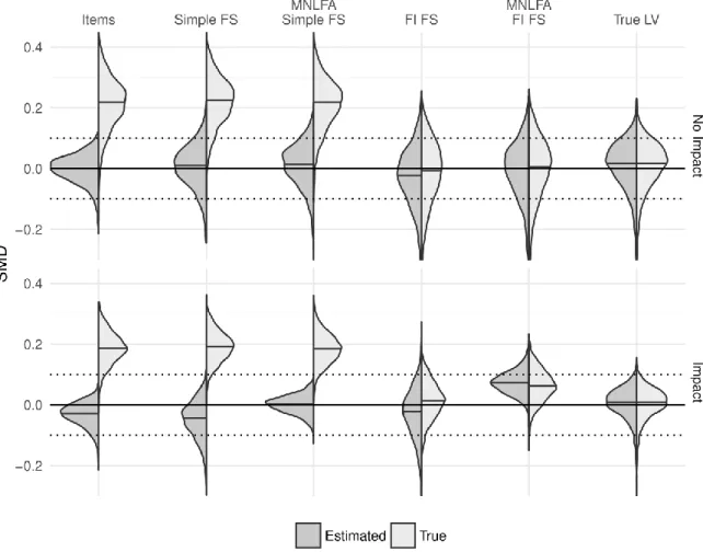
For each method, estimated and true balance summaries were created. For the methods that involved estimating a factor score, the estimated balance summary was the weighted SMD of the factor scores, computed as in equation (9). For the Items method, which did not involve
estimating a factor score, the average weighted SMD of the items was used as the estimated balance summary. For all methods, the true balance summary was the weighted SMD of the true LV using the weights estimated with that method. For each method and design cell, the average true balance summary was computed to examine the degree to which the estimated weights balanced the true LV; this are reported as the mean SMD of the true LV. Values close to 0 indicate good balance in the variable means between the treatment groups; authors recommend ensuring weighted SMDs below 0.1 before proceeding with effect estimation.
In addition, the RMSBD was computed as the square root of the mean squared difference
5 For each method, I computed an analogue to the pooled standard error of the PBR and multiplied by 2; for all
between the true and estimated balance summaries for each method and cell; this value represents the typical difference between the estimated balance summary, which would be accessible to researchers, and the true balance summary, which is normally inaccessible but which is desired. Values of the RMSBD close to 0 indicate that the estimated balance summary is similar to the true balance summary and might be used as a proxy for measuring balance on the true LV. Values of the RMSBD larger than 0.1 are particularly problematic because they indicate that even after achieving perfect balance based on the estimated balance summary, problematic imbalances in the true LV are likely to remain.
CHAPTER 2: RESULTS
First, I discuss issues of model convergence and aberrant estimates. Next, I discuss the quality of the factor scores and propensity scores. Next, I discuss the bias and variability for each method in terms of mean PBR and RMSPBR across conditions. Finally, I discuss the balancing performance of the methods with respect to the mean true balance and RMSBD.
Convergence and Aberrant Estimates
I fit a total of 32,000 factor models across all replications and conditions: four scoring models (simple FA model, simple MNLFA model, fully inclusive FA model, and fully inclusive MNLFA model) fit to 1,000 replications within each of 8 cells6. Fourteen models failed to converge, yielding model parameter estimates that were not true maximum likelihood solutions: nine occurred in estimating the simple MNLFA models, and five occurred in estimating the fully inclusive MNLFA models. The failures only occurred when DIF was present and with six items. I omitted results originating from these models from all subsequent analyses.
All replications were checked for impossible or unusual parameter values, outlying data points, and extreme effect estimates. Although there were some unusual parameter estimates and effect estimates, these were not deemed to be worthy of removal because they appeared to be the result of natural randomness or estimation uncertainty that was relevant to the analysis.
Score Quality
I computed correlations between the estimated factor score and the true LV values and between the estimated propensity scores and the optimal propensity scores to inform variations in other criteria presented below. Correlations close to 1.00 indicate high score quality,
suggesting performance of the scores close to their respective benchmarks. First, I discuss the quality of the estimated factor scores, and then I discuss the quality of the estimated propensity scores. Across both sets scores, patterns were similar regardless of the number of items, so only the six-item conditions will be discussed.
Factor Scores. The distributions of correlations between the estimated factor scores and the
true values of the LV are displayed in the top panel of Figure 4. The largest differences were between the unconditional factor scores and the MNLFA-based factor scores. In the absence of impact and DIF, all factor score performed similarly with mean correlations around .83,
indicating fairly good agreement with the true LV values. In the presence of impact and DIF, the unconditional factor scores had mean correlations around .77, while the MNLFA-based factor scores had mean correlations around .84. Similar results were found in Curran et al. (2016), in which MNLFA-based factor scores were more highly correlated with true LV values than were unconditional scores in the presence of impact and DIF, especially when impact and DIF effects were strong. The fully inclusive factor scores were consistently slightly more correlated with the true factor scores on average (by a small margin of approximately .005), as these factor scores were effectively computed with an additional correctly modeled indicator (i.e., the treatment).
Propensity Scores. The distributions of correlations between the propensity scores estimated
though some patterns emerged: overall, the simple FS and MNLFA simple FS methods yielded higher mean correlations than did using the items or the fully inclusive methods. Across
conditions, the MNLFA simple FS yielded higher mean correlations than the other methods, ranging from .96 in the absence of impact and DIF to .97 in the presence of both. The
unconditional fully inclusive FS consistently yielded the lowest mean correlations, ranging from .94 in the presence of impact and DIF to .95 in the absence of both, despite the method’s high performance on the other metrics described below.
Bias and Variability of Effect Estimates
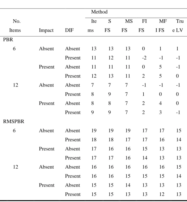
Mean PBR and RMSPBR values are displayed in Figure 5 and detailed in Table 3. Across cells and models, there was substantial variability in mean PBRs: values ranged from -2 to 13 (i.e., between -2 and 13 percent of the original bias remaining). On the other hand, RMSPBRs were not highly variable: values ranged from 12 to 19 (i.e., the typical PBR was between 12 and 19 percentage points from 0 percent). Given that mean PBRs for some methods and cells were close to 0, these methods were able to yield mostly unbiased estimates. Performance of each method on these metrics in the various conditions of impact, DIF, and number of items is described below. First, I describe the performance of the simple methods (those that do not involve including the treatment in the factor score model), and next I describe the fully inclusive methods.
treatment.
With six items and no impact or DIF, using the items directly yielded a mean PBR of 13, indicating significantly biased effect estimates. Surprisingly, the presence of impact or DIF slightly improved bias removal; with either impact or DIF present, the mean PBR was 11, and with both, the mean PBR was 12. The opposite pattern emerged with 12 items: the least bias was observed when neither impact nor DIF were present (mean PBR = 7), and the greatest bias was observed when both impact and DIF were present (mean PBR = 9). Regardless of the presence of impact or DIF, using the items yielded biased effect estimates, especially with fewer items.
The RMSPBR largely remained the same or decreased in the presence of impact or DIF. With six items, RMSPBR was 19 in the absence of impact and DIF, 18 in the presence of only DIF, 17 in the presence of only impact, and 17 in the presence of both impact and DIF,
indicating large typical differences between the estimated treatment effect and the true effect. With 12 items, RMSPBR was 16 in the absence of impact (regardless of DIF) and 15 in the presence impact (regardless of DIF). The bias and RMSPBR patterns were in approximately the same direction with six items, but in opposite directions with 12 items.
Simple Factor Score. The simple FS method involved estimating factor scores from an unconditional measurement model that included the items as indicators of the LV (Figure 3A). In the presence of impact, this method was incorrect in assuming an unconditional normal
distribution for the LV when in reality the distribution was conditional on the covariates7. In presence of DIF, this method was incorrect in assuming equal intercepts and loadings for each item across all units, when in reality these parameters of the measurement equations varied
7 Note that in the “Impact absent” condition, the LV distribution was also normal only conditional on the covariates,
across units based on their covariates values.
The bias and RMSPBR results for the simple FS method were almost identical to those from the items, echoing the results of Nguyen et al. (under review), and indicating similarly significant bias in the effect estimates. With six items, the mean PBR was 13 in the absence of impact and DIF, 12 in the presence of only DIF, 11 in the presence of only impact, and 13 in the presence of both impact and DIF. With 12 items, the mean PBR was 7 in the absence of impact and DIF, 9 in the presence of only DIF, 8 in the presence of only impact, and 9 in the presence of both impact and DIF. The RMSPBR results were identical to those using the items method, except that in the presence of only impact with six items, the simple FS method yielded an RMSPBR of 15. In general, using the simple factor score yielded similar bias and RMSPBR to using the items; when the methods differed, the simple FS method always yielded increased bias compared to using the items, but these differences were only by one point8. The relatively high mean PBR and
RMSPBR results indicate significant bias in treatment effect estimates and that effect estimates were typically quite far from the true effect.
MNLFA Simple Factor Score. The MNLFA simple FS incorporated the covariate effects on the LV distribution and measurement equations into the scoring model but did not include the treatment variable as an indicator (Figure 3B). When both impact and DIF were present, this method matched the data-generating process for the LV and its indicators; when either were absent, this method over-modeled nonexistent relationships between the covariates and the LV distribution and measurement equations.
Overall, the MNLFA simple FS method yielded mean PBR and RMSPBR values similar to or slightly less than those from using the items or using the (unconditional) simple FS. In the