RISK POOLING TO MITIGATE HYDROLOGY-RELATED FINANCIAL LOSSES FOR WATER UTILITIES
Rachel Baum
A dissertation submitted to the faculty at the University of North Carolina at Chapel Hill in partial fulfillment of the requirements for the degree of Doctor of Philosophy in the Department
of Environmental Sciences and Engineering in the Gillings School of Global Public Health.
Chapel Hill 2019
Approved by:
Gregory Characklis
Jon Herman
Jeff Hughes
Marc Serre
© 2019 Rachel Baum
ABSTRACT
Rachel Baum: Risk Pooling to Mitigate Hydrology-Related Financial Losses for Water Utilities (Under the direction of Gregory Characklis)
conditions in which droughts are subject to some level of spatial autocorrelation, has the
potential to significantly reduce the insurer’s required reserves, and thereby the opportunity costs of maintaining them, resulting in lower contract costs for water utilities. Chapter 3 builds upon the findings of Chapter 2, and assesses strategies for further cost reduction measures through integrating PHDI-based index insurance with reinsurance purchased from a third party, which can reduce the net cost of risk management for utilities over both individual and multi-year periods. Chapter 4 addresses the challenges associated with lowering the basis risk inherent in broadly applicable index insurance contracts through multi-variate indices derived from decision tree-based models, with multiple indexes considered using different spatial and temporal
resolutions. Index contracts developed from these tree-based models are found to substantially reduce basis risk, increasing the effectiveness of index insurance and making them more
attractive to both buyers and sellers. Overall, this dissertation demonstrates the potential benefits, while addressing some of the primary challenges, of using financial instruments to pool
TABLE OF CONTENTS
LIST OF TABLES………... viii
LIST OF FIGURES………... ix
CHAPTER 1: INTRODUCTION ………... 1
1.1 INTRODUCTION …….……….………...…….…………... 1
REFERENCES …….……….………...…….……….……….... 7
CHAPTER 2: EFECTS OF GEOGRAPHIC DIVERSIFICATION ON RISK POOLING TO MITIGATE DROUGHT RELATED FINANCIAL LOSSES FOR WATER UTILITIES ……….………... 10
2.1 INTRODUCTION.……….………...…….……….……… 10
2.2 METHODS ………….…….……….………...…….……….. 16
2.2.1 Identifying an effective index ……… 21
2.2.2 Hydrologic indices and correlation with operating revenue……….. 23
2.2.3 Sharing risk through spatial diversification……… 28
2.2.4 Determining the effects of risk pooling………..31
2.3 RESULTS ....……….………...…….……….………... 38
2.4 DISCUSSION ....……….………...…….……….………... 45
2.5 CONCLUSION.….……….………...…….……….……… 47
REFERENCES.….……….………...…….……….………... 49
3.1 INTRODUCTION.……….………...…….……….……… 54
3.2 METHODS ………….…….……….………...…….……….. 59
3.2.1 Generating synthetic PHDI data….……… 60
3.2.2 Designing index-based insurance contracts……….………. 65
3.2.3 Pricing index insurance contracts……….……….. 69
3.2.4 Designing reinsurance contracts……….……… 70
3.2.5 Pricing reinsurance contracts.……….……… 71
3.2.6 Determining risk exposure with reinsurance……….………. 76
3.3 RESULTS ....……….………...…….……….………... 77
3.3.1 Average Net Cost for mutual members……….………. 78
3.3.2 Total Net Cost for mutual members over ten years……… 80
3.4 DISCUSSION ....……….………...…….……….…….….. 84
3.5 CONCLUSION.….……….………...…….……….……… 86
REFERENCES.….……….………...…….……….………….. 88
CHAPTER 4: USING TREE-BASED MODELS TO REDUCE BASIS RISK IN INDEX-INSURANCE CONTRACTS DESIGNED TO MANAGE FINANCIAL RISKS RELATED TO HYDROLOGIC VARIABILITY …….………... 95
4.1 INTRODUCTION.……….………...…….……….……… 95
4.2 METHODS ………….…….……….………...…….………... 101
4.2.1 Measuring contract and model performance...………..………... 102
4.2.2 Univariate index-based insurance contract design………... 105
4.2.3 Multivariate tree-based index-based insurance contract design…………... 107
4.2.4 Contract pricing ………... 115
4.3.1 Individual utility performance………...………..………... 127
4.4 DISCUSSION ....……….………...…….……….………... 129
4.5 CONCLUSION....……….………...…….……….……… 130
REFERENCES....……….………...…….……….………..… 132
CHAPTER 5: CONCLUSIONS AND FUTURE WORK………... 137
LIST OF TABLES
Table 1. Data characteristics for each tested index………....……….……... 25
Table 2. Utility groupings measured by correlation between index and operating revenues…… 27
Table 3. Reinsurance contract prices and loadings for various attachment points and a limit of $212M (99.5% VaR) and associated annual amortized debt service costs.……… 74
Table 4. Data and sources for predictor variables ………...…….………... 111
Table 5. Optimal parameters for each tree-based algorithm …………....……….. 117
Table 6. Importance ranks for each model …….…………....………...120
Table 7. Comparison of contrat performance in terms of basis risk metrics ………... 123
Table 8. Comparison of results between all models ……….. …………....……… 125
LIST OF FIGURES
Figure 1. Generic index-based insurance payout function….……….... 17
Figure 2. Illustrative example of the effects of covariance on VaR: When spatial
autocorrelation increases (i.e. the level of independence decreases), the VaR increases……….. 20
Figure 3. Locations for the 315 utilities used in this study (divisions indicate
NOAA climate division boundaries) ….………... 21
Figure 4. Covariance of streamflow (top) and PHDI (bottom) values corresponding to 143 (streamflow) and 245 (PHDI) utilities that exhibit some correlation (>0)
between the index and revenues………... 30
Figure 5. Identifying the strike, slope, and distribution of payouts characterizing each utility…. 33
Figure 6. 99.5% VaR comparison across different utility risk levels for the
group of insured utilities with indices related to streamflow (left) and PHDI (right)…………... 38
Figure 7. Opportunity costs of maintaining larger liquid reserves for risk pooling
versus risk shifting for streamflow-based contracts (left) and PHDI-based contracts (right)... 40
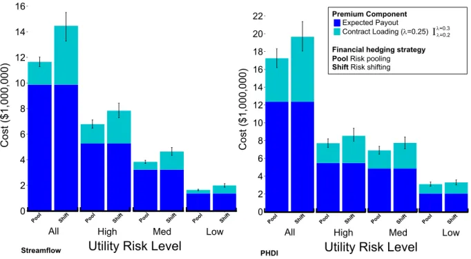
Figure 8. Expected payout and contract loading costs for risk shifting and risk
pooling for streamflow (left) and PHDI (right) contracts... 41
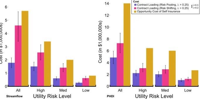
Figure 9. Opportunity cost of self-insurance versus contract loading costs under
different levels of risk and insuranc strategy... 43
Figure 10. Total payouts, premiums, and reserves over the synthetic period
1970-2014 for the streamflow-indexed insurance contracts……….. 44
Figure 11. Flow of funds for insuring with and without reinsurance... 56
Figure 12. Number of autoregressive lags determined to be significant for
each climate division... 63
Figure 13. Annual PHDI data for all 344 climate divisions for historic data
(from 1895-2015) and synthetic data (100,000 years).……….. 64
Figure 14. Current populations served by publicly operated surface water
utilities for each of 344 climate divisions ……….……… 66
Figure 15. Generic structure of PHDI-indexed insurance payout with a strike of -3…………... 67
Figure 16. Distribution of the annual payouts for the risk pool and the highest
Figure 17. Modeled catastrophe bond prices based on the Braun pricing
model compared to historic actual prices ……….…….………...75
Figure 18. Tradeoff between annual reinsurance loading and debt service costs for insuring with reinsurance at various attachment points compared to insuring without reinsurance. The lower and upper bounds (dashed lines)
around reinsurance loading indicate +/- 10% sensitivity limit…………...………... 79
Figure 19. Net Cost (annual) for insuring with reinsurance at various attachment points compared to insuring without reinsurance. The lower and upper bounds
(dashed lines) indicate +/- 10% sensitivity limits... 80
Figure 20. Net Cost across 10-years for insuring with and without reinsurance,
beginning at a $130M attachment point when insuring with reinsurance………... 81
Figure 21. Reserves after 10-years for insuring with and without reinsurance,
beginning at a $130M attachment point when insuring with reinsurance ………... 82
Figure 22. Net reserves after 10-years for insuring with and without reinsurance,
beginning at a $130M attachment point when insuring with reinsurance ………...84
Figure 23. Index-based insurance contract with low basis risk (left) versus
an index-based insurance contract with higher basis risk (right) ………... 97
Figure 24. Locations for the 325 water utilities assessed in this study.…………... 102
Figure 25. Illustrative figure demonstrating the categories of outputs
(underpayment, overpayment, anticipated payment) ………..……….... 104
Figure 26. Univariate index-based insurance contract design.………... 106
Figure 27. Machine learning model development steps for each tree-based algorithm……….. 107
Figure 28. Generic decision tree design .………... .………... 108
Figure 29. Decision tree results indicating predictors (f), threshold (t) values,
and standard normalized payouts (µ=0, s=1)………..………….... 118 Figure 30. Comparison of results between the baseline univariate PHDI model
and the tree-based multivariate models ……….……….121
Figure 31. Performance comparison of contracts based on the baseline (PHDI) and tree-based models for the subset of 92 utilities exhibiting high correlation
Figure 32. Distribution of aggregate annual payouts based on synthetic
scenarios involving contracts derived from the baseline and tree-based models,
as well as annual payouts derived from historic data (2003-2013) ………... 126
Figure 33. Distribution of root mean square error of payouts across utilities for
CHAPTER 1: INTRODUCTION
Hydrologic variability poses serious challenges to effective water supply management
(Chapman, 2012; National Research Council, 2011; Polasek, 2014; The World Bank, 2009).
While the maintenance of surplus supply capacity (beyond that required to meet demands under
average conditions) has historically served as a successful hedge against drought events, the
declining availability of new supplies, higher costs, and a more onerous environmental approval
process have all served to reduce the pace of new source development. (FEMA, 2012; Gleick,
2003; Ho et al., 2017; Kundzewicz et al., 2007; GWSP Digital Water Atlas, 2018). As a result,
many water utilities have begun to rely more heavily on nonstructural alternatives, including
various forms of demand management (i.e. conservation) and reallocation of existing supplies
(i.e. water transfers) as a means of managing drought (Beecher and Chesnutt, 2012; Brajer et al.,
1989; Leurig, 2010; U.S. Army Corps of Engineers, 1994). These approaches have often been
effective, but can also lead to significant variability in utility costs and revenues (Donnelly and
Christian-Smith, 2013; Hughes et al., 2014; Schmidt and Lewis, 2017; Tiger et al., 2014). These
unpredictable variations introduce financial instability, which is difficult for utilities to manage,
given their typical budgetary model in which prices are set to recover costs, and exacerbated by
their financial structure in which the majority of costs are fixed (e.g., debt service) while the
majority of revenues are linked to water sales (Donnelly and Christian-Smith, 2013; Olmstead
and Stavins, 2009; Schmidt and Lewis, 2017; Spang et al., 2015). As such, unexpected
decreases in costs. Unexpected increases in costs due to drought management activities (e.g.,
water transfers) introduce similar challenges. Both activities can lead to budget shortfalls that can
be difficult to mitigate, as raising prices quickly enough to compensate for lost
revenues/increased costs is often infeasible for these heavily regulated public sector
organizations (Hughes et al., 2014; Olmstead and Stavins, 2009; Tiger et al., 2014). In terms of
impact, financial instability can lead to a host of challenges, not least of which is a credit rating
downgrade, which can significantly increase borrowing rates (Chapman, 2017; Donnelly and
Christian-Smith, 2013; Polasek, 2014). For a capital-intensive sector like the water utility
industry, in which the majority of costs typically come in the form of debt service payments,
credit downgrades can present significant and long-term financial challenges for water utilities
(Hughes et al., 2014; Leurig, 2012).
Mitigating the financial consequences of hydrologic variability can be accomplished via a
number of approaches including drought surcharges, changes in pricing regime (e.g., fraction of
fixed vs. volumetric) (Schmidt and Lewis, 2017; Spang et al., 2015),and the maintenance of
reserve funds (Donnelly and Christian-Smith, 2013). Additionally, recent studies have found that
financial instruments may also have significant potential in mitigating these financial
consequences (Zeff et al., 2014; Zeff and Characklis, 2013). Instruments such as index insurance
that provide financial payouts under water scarce conditions are one example. In this case, the
payout amount is linked to specified thresholds measured by an index composed of one or more
metrics (e.g. precipitation) rather than a direct assessment of damages. In order to be effective,
the index must exhibit a high correlation with financial losses, a situation in which the contracts
are characterized as having low “basis risk”. Examples include index insurance based on the
power industry (where the majority of demand comes from heating/cooling of buildings) and
dryland agriculture where precipitation and crop yields can be closely linked (Cao and Wei,
2004; Fuchs and Wolff, 2011; Müller and Grandi, 2000; Stoppa and Hess, 2003; Turvey, 2001;
Varangis et al., 2001).
Financial contracts have been explored in the literature as a means of transferring the
financial risk of drought from an individual water utility to a third-party insurer (i.e. risk shifting)
(Brown and Carriquiry, 2007; Zeff and Characklis, 2013; Zeff et al., 2014) using contracts based
on indices carefully constructed for an individual utility’s circumstances. However, these indices
can be time consuming and expensive to develop, limiting the commercial viability of
developing indices tailored to many individual utilitity’s circumstances. Moreover,
individualized contracts can result in the insurer having to maintain higher reserves in order to be
able to ensure payouts under extreme conditions. The opportunity costs of maintaining these
reserves in a liquid (i.e. rapidly accessible) form, in which lower returns are earned, can be quite
high.
To reduce the opportunity costs of capital and encourage broader adoption of a financial
instrument, risk pooling via a generalized form of index-based contracts may have significant
potential. Risk pooling involves the sharing of uncorrelated, or mostly uncorrelated, risks, which
reduces the probability of all the insured parties experiencing a loss at the same time, thereby
reducing the capital reserves needed to make payouts to those parties with a specified level of
confidence. As more parties join the risk pool, the average losses for the pool converge to the
expected losses (Law of Large Numbers) and the variance of the average of pooled losses
decreases (Central Limit Theorem) (Smith and Kane, 1994). This translates into lower
member. However, weather events, such as drought, are spatially autocorrelated
(non-independent), potentially reducing the effectiveness of risk pooling relative to an ideal scenario
(uncorrelated risks), but the degree to which this occurs is still undetermined.
This dissertation assesses the potential advantages of pooling drought-related financial
risks across the U.S. through hydrologic-based index insurance. The objectives are to better
understand the challenges, such as the spatial autocorrelation of drought, and high levels of basis
risk, while also developing various insurance contract designs that could lead to more effective
financial insurance for protecting water utilities from drought-related losses. Chapter two
(recently published in Water Resources Research (Baum et al., 2018)), examines the potential of various indices to serve as a basis for contracts, and then analyzes the spatial autocorrelation of
these indices to describe the benefits of risk pooling, as measured by the reduction in reserve
requirements and consequent lowering of the opportunity costs of capital that can lead to lower
insurance prices. This analysis focuses on a group of 315 utilities, for which a unique set of
financial data was available. This work then uses these utilities to quantify the reduction in costs
of managing financial risks of droughts via risk pooling, relative to a situation in which a utility
would engage with an insurer in a single contract (risk shifting) or seek to self-insure by
maintaining sufficient reserves of its own. Results suggest that risk pooling has the potential to
significantly lower required reserve levels and reduce the contract costs, however there are still
extreme (low probability, high consequence) events to which these utilities are exposed that
contribute to driving reserve requirements significantly higher than they would otherwise be.
Chapter 3 addresses the financial challenges that these extreme risks pose for risk pools
and analyzes strategies for reducing risk management costs through the additional use of risk
and Management). Reinsurance involves the transfer of specified risks from an insurer or mutual (essentially an insurance firm owned and operated by the insured parties) to a reinsurer that
typically uses diversification across a portfolio of large but uncorrelated risks, to reduce the
required reserves needed to compensate its counterparties (e.g., insurance firms or mutual),
taking advantage of its lower costs of capital to assume risks for lower cost than the
counterparties themselves (Schanz et al., 2010; Scordis and Steinorth, 2012). This analysis
assesses the advantages of reinsurance in reducing capital costs, when layered with risk pooling,
and describes how a combination of risk pooling and risk shifting can further reduce the costs of
achieving an equivalent level of financial protection for a national-scale pool (i.e. mutual) of
water utilities over both individual and multi-year periods.
While each member of a risk pool benefits from the lower costs of managing risk via a
combination of pooling and shifting, each is also ultimately responsible for its own financial
stability. Therefore, each pool member (i.e. water utility) will be concerned with how effective
index insurance, or any financial instrument, is in reducing its own financial risks. A water utility
will only find a financial instrument to be attractive if it provides adequate protection at a
reasonable price and exhibits low basis risk. Compared to an individualized contract, the basis
risk associated with the generalized contract is likely to be greater. In order to reduce the basis
risk of the generalized contracts developed for risk pooling applications, Chapter 4 develops a
generalized decision tree-based model in which multi-variate indices are used to determine
payouts. While many existing parametric contracts are based on a single index, this work aims to
use multivariate indices to better account for the individual circumstances of different water
utilities that may complicate the correlation between any one index and utility revenues. This
identifying contract structures with lower basis risk, one that should be easily scalable to a
national level. Lowering basis risk in this way increases the probability of each water utility
receiving an appropriate payout when experiencing hydrologic-related losses, increasing the
likelihood of more utilities participating in the risk pool.
Hydrologic variability is predicted to increase in the future (National Drought Mitigation
Center, 2016), and combining this with projections of increased water demand and growing
barriers to new supply development, suggests new approaches will be required to promote
financially stable water utilities. Given the negative effects of low revenue years, and the
increasing rate of credit ratings downgrades among utilities (Donnelly and Christian-Smith,
2013), it is clear that water utilities face long-term financial challenges as a result of hydrologic
variability. This dissertation develops novel financial instruments and more sophisticated risk
management strategies for water utilities that are vulnerable to weather-related financial losses.
Given the success of other economic sectors in using financial instruments to reduce
weather-related losses and the potential to create less expensive financial instruments with low basis risk,
there is great potential for widespread scalability of improved financial risk management for
water utilities via risk pooling. Improved strategies could benefit thousands of water utilities,
providing them with greater financial stability, and ultimately lower prices to utility customers
over the long-term. The tools and strategies developed in this work may also bring insights that
can be applied more broadly to other economic sectors facing weather-based financial volatility
REFERENCES
Baum, R., Characklis, G. W., and Serre, M. L. (2018). Effects of Geographic Diversification on Risk Pooling to Mitigate Drought-Related Financial Losses for Water Utilities. Water Resources Research, 1–19. https://doi.org/10.1002/2017WR021468
Beecher, J. A., and Chesnutt, T. W. (2012). Declining Water Sales and Utility Revenues: A Framework for Understanding and Adapating. Racine, WI.
Brajer, V., Church, a L., and Cummings, R. (1989). The Strengths and Weaknesses of Water Scarcity and Sovereignty. Natural Resources Journal, 29, 489–509.
Brown, C., and Carriquiry, M. (2007). “Managing hydroclimatological risk to water supply with option contracts and reservoir index insurance.” Water Resources Research, 43.
Cao, M., and Wei, J. (2004). Weather Derivatives: A New Class of Financial Instruments, 1–26.
Chapman, T. (2012). From Droughts to Conservation: Water Can Have Big Effects on U.S. Municipal Utility Credit Rating. CreditWeek, 32(9), 33–37. Retrieved from
http://www.standardandpoors.com/spf/swf/water/data/document.pdf
Chapman, T. (2017). U.S. Municipal Water Utility Sector 2017 Outlook: Potholes, Policies, and Pensions, 1–8.
Donnelly, K., and Christian-Smith, J. (2013). An Overview of the “New Normal” and Water Rate Basics. Pacific Institute, 1–23. Retrieved from
http://www.pacinst.org/wp-content/uploads/2013/06/pacinst-new-normal-and-water-rate-basics.pdf
FEMA. (2012). United States Dam Inventory Data, (July).
Fuchs, A., and Wolff, H. (2011). Concept and unintended consequences of weather index insurance: The case of mexico. American Journal of Agricultural Economics, 93(2), 505– 511. https://doi.org/10.1093/ajae/aaq137
Gleick, P. H. (2003). Global Freshwater Resources: Soft-Path Solutions for the 21st Century. Science, 302(5650), 1524–1528. https://doi.org/10.1126/science.1115233
Ho, M., Lall, U., Allaire, M., Pal, I., Raff, D., Wegner, D., … Kwon, H. H. (2017). The future role of dams in the United States of America Michelle. Water Resources Research, 982– 998. https://doi.org/10.1002/2016WR019905.Received
Kundzewicz, Z. W., Mata, L. J., Arnell, N. W., Döll, P., Kabat, B., Jimenez, B., … Editors, R. (2007). Freshwater resources and their management. World Water, 173–210.
https://doi.org/10.1017/CBO9781107415324.004
Leurig, S. (2010). The Ripple Effect: Water risk in the municipal bond market. Ceres. https://doi.org/10.1073/pnas.1005764107/-/DCSupplemental
Leurig, S. (2012). Water Ripples: Expanding Risks for U.S. Water Providers. Ceres Report, (December).
Müller, A., and Grandi, M. (2000). Weather Derivatives: A Risk Management Tool for Weather-sensitive Industries. The Geneva Papers on Risk and Insurance, 25(2), 273–287.
https://doi.org/10.1111/1468-0440.00065
National Research Council. (2011). Global Change and Extreme Hydrology: Testing Conventional Wisdom. National Academies Press. https://doi.org/10.17226/13211
Olmstead, S. M., and Stavins, R. N. (2009). Comparing price and nonprice approaches to urban water conservation, 45(March), 1–10. https://doi.org/10.1029/2008WR007227
Polasek, J. (2014). Sustainable Utilities: Financial Instruments to Manage Weather-Related Revenue Risk. Chicago, IL.
Schanz, K.-U., Fehr, K., and Armitage, T. (2010). The essential guide to reinsurance, 51.
Schmidt, A., and Lewis, L. (2017). The Cost of Stability: Consumption-Based Fixed Rate Billing for Water Utilities, (160), 5–24.
Scordis, N. A., and Steinorth, P. (2012). Value from Hedging Risk with Reinsurance. Journal of Insurance Issues, 35(2), 210–231.
Spang, E. S., Miller, S., Williams, M., and Loge, F. J. (2015). Consumption-based fixed rates: Harmonizing water conservation and revenue stability. Journal - American Water Works Association, 107(3), E164–E173. https://doi.org/10.5942/jawwa.2015.107.0001
Stoppa, A., and Hess, U. (2003). Design and Use of Weather Derivatives in Agricultural Policies: The Case of Rainfall Index Insurance in Morocco.
The World Bank. (2009). Water and Climate Change : Understanding the risks and making Climate-smart investment deCisions. DC World Bank, 2(November), 174.
Tiger, M., Hughes, J., and Eskaf, S. (2014). Designing Water Rate Structures for Conservation and Revenue Stability.
U.S. Army Corps of Engineers. (1994). Managing Water for Drought. IWR Report 94-NDS-8, 210. Retrieved from
http://drought.unl.edu/portals/0/docs/ManagingWaterForDrought.pdf%0Ahttp://www.iwr.u
sace.army.mil/Portals/70/docs/iwrreports/94nds8.pdf%5Cnhttp://library.water-resources.us/pubsearchS.cfm?series=NDS
Varangis, P., Skees, J., and Barnett, B. (2001). Weather Indexes for Developing Countries. Climate Risk and the Weather Market, 1–16.
Zeff, H. B., and Characklis, G. W. (2013). Managing water utility financial risks through third-party index insurance contracts. Water Resources Research, 49(8), 4939–4951.
https://doi.org/10.1002/wrcr.20364
Zeff, H. B., Kasprzyk, J. R., Herman, J. D., Reed, P. M., and Characklis, G. W. (2014). Navigating financial and supply reliability tradeoffs in regional drought management portfolios. Water Resources Researchesources, 50, 4906–4923.
CHAPTER 2: EFECTS OF GEOGRAPHIC DIVERSIFICATION ON RISK POOLING TO MITIGATE DROUGHT RELATED FINANCIAL LOSSES FOR WATER
UTILITIES1
2.1INTRODUCTION
Many regions across the United States face increasing vulnerability to drought due to
growing demands and constraints on supply development (e.g. reduced availability,
environmental permitting), with an average of 9% of the country experiencing severe drought at
any given time since 2000 (National Drought Mitigation Center, 2016). The challenges
associated with expanding and/or maintaining large supply capacities as a hedge against drought
events have led many utilities to rely more heavily on non-structural alternatives to manage
drought, such as temporary conservation measures (Leurig, 2010; Brajer et al., 1989; Alliance
for Water Efficiency, 2012). While this alternative has proven effective for ensuring a high level
of reliability (Alliance for Water Efficiency, 2012), it introduces financial instability in the form
of lower revenues that can make temporary conservation measures less attractive to utility
managers.
Water utility finances are structured in such a way that short-term costs are mostly fixed
(~80-95%), much of this due to debt service payments on infrastructure, while most revenues
(~80-90%) are generated via volumetric water sales (Hughes et al., 2014; Hanemann, 1997).
However, in the long-term, costs are variable as the system depreciates and capacities change
1Published in Water Resources Research. Baum, R., Characklis, G. W., and Serre, M. L. (2018). Effects of
geographic diversification on risk pooling to mitigate drought-related financial losses for water utilities. Water
(Hanemann, 1997). This work is focused on management of short-term variability in revenues due to drought, which leads to unpredictable reductions in usage, as a result of drought-related
conservation measures. This disrupts a utility’s traditional cost recovery budgetary model,
wherein prices are set such that revenues are expected to equal costs at the end of each budgeting
period, typically annually (Hughes et al., 2014; Tiger et al., 2014). Disruptions are difficult to
remedy in the short-run as prices for publicly operated utilities cannot be quickly or easily
modified. Across the U.S., water utility financial health, as measured by metrics such as debt
service coverage ratio (revenues divided by debt service obligations), has been declining, as
greater reliance on demand management has resulted in an increased frequency of lower revenue
periods (Alliance for Water Efficiency, 2014). Given that raising prices to compensate for lower
revenues can be politically difficult (Olmstead and Stavins, 2009), even a five percent reduction
in revenue can be challenging to manage (Zeff et al., 2014). Water utilities are also concerned by
events that reflect poorly in their financial metrics, as this can lead to credit downgrades. A credit
downgrade can significantly increase the rate at which a utility borrows, a critically important
factor in this capital intensive sector where debt-service costs can account for up to 50% of a
utility’s total costs (Hughes et al., 2014). These pressures have contributed to a situation in which
5% of the rated utilities across the country received credit rating downgrades in 2016 (Chapman
et al., 2017).
In order to avoid budget shortfalls and credit downgrades, some water utilities are
shifting away from volumetric pricing toward higher fixed charges in order to stabilize their
revenue stream. However, this reduces consumers’ incentives to conserve, further exacerbating
short-term water scarcity concerns from drought events and contributing to the long-term
for promoting financial stability, alternative strategies to maintain utility financial stability are
also being explored.
Beyond changing prices, utilities have several alternatives for achieving greater financial
stability during times of severe drought, each with strengths and weaknesses. Drought surcharges
can compensate for fluctuations in revenues and costs, but are often unpopular with consumers
who are typically already being asked to conserve. Furthermore, inelastic urban water demand
often means that these surcharges must be substantial in order to achieve the desired level of
conservation (Tiger, 2009; Zeff and Characklis, 2013). Contingency, or “rate stabilization”,
funds can act as a form of self-insurance with a utility contributing regularly to such a reserve
and drawing on it during times of severe drought. However, the size of this reserve and the
opportunity costs of maintaining it (e.g. low returns on liquid reserves) can grow quite large if
the utility seeks to protect itself against more extreme events, and even larger if used to protect
against a multi-year drought, or several droughts over a small span of years. Additionally,
utilities associated with city government may also have difficulty maintaining such a reserve, as
it would be an attractive target for other community spending priorities (Tiger, 2009; Eskaf et al.,
2014).
Given the challenges in existing solutions to protect utilities from revenue variability due
to drought and the growing need for solutions that align with temporary actions, such as
conservation, another alternative solution has recently been proposed, one that has been used in
many other contexts, but is relatively new to water utilities, that of financial insurance. Financial
insurance contracts, often in the form of index insurance, have been developed to mitigate
environmental financial risks in a number of other contexts. These include contracts designed to
Cao and Wei, 2004), low rainfall (Turvey, 2001; Varangis et al., 2001; Procom et al., 2003;
Martin et al., 2001; Fuchs and Wolff, 2011), and low streamflow (Foster et al., 2015; Meyer et
al., 2015), with application in the electric utility, agriculture, and hydropower sectors, among
others. The success of these index insurance contracts in other contexts, coupled with the
increased need for new solutions to deal with increasingly volatile weather, has increased the
motivation for creating financial instruments (Alliance for Water Efficiency, 2014; Eskaf et al.,
2104; Chesnutt et al., 2014).
This research explores financial contracts that would provide water utilities with a
payout when pre-specified drought conditions prevail (Brown and Carriquiry, 2007; Zeff and
Characklis, 2013). These financial contracts transfer some of the financial risk of drought events
to a third party or mutual in exchange for some form of payment (i.e. premium). The third party
might be a large financial institution, capable of either taking on the risk exposure of the
individual utility (risk shifting), or seeking to organize and manage a pool of similar (presumably
spatially uncorrelated) risks. Alternatively, a group of utilities with similar risks could
self-assemble to pool risks through some form of mutual. The advantages of pooling uncorrelated
risks via either approach (third party or mutual) can lead to lower risk management costs as they
reduce the size of required reserves relative to either self-insurance (e.g. contingency fund) or
risk shifting to a third party on an individual basis, and thereby lower opportunity costs of
maintaining large liquid reserves (i.e. those that can be accessed easily at any time). For all of
these insurance approaches, the premium paid for the insured party is computed based on the
expected payout to the covered party (i.e. utility) plus an additional “loading”, which accounts
As an insurance tool for water utilities, third party indexed contracts have shown some
promise, particularly as part of an integrated financial risk management strategy (Zeff and
Characklis, 2013, Zeff et al., 2014). Zeff et al. found that index-based financial contracts have a
critical role to play in optimal financial risk management portfolios (which also include
restrictions, transfers, and contingency funds), being a necessary part of the portfolio in order to
carry out the operational goals and maintain financial stability of the utility. Thus far, however,
these contracts have been designed for the relatively specialized circumstances of a single utility
and developing a utility-specific index requires considerable time and localized information to
develop, raising costs and limiting the potential for widespread implementation (Zeff and
Characklis, 2013; Zeff et al., 2014; Zeff et al., 2016). A more generalized form of index
insurance contracts, one linked to a broadly available metric, would facilitate the pooling of risks
across many utilities, lowering both transaction costs and the price of the contracts (Wang and
Zhang, 2003).
In its purest sense, risk pooling involves parties with similar, but independent, risks (e.g.
automobile collisions) contributing to a collective fund from which each affected party can draw
when it experiences a loss. The independence of the risks makes the probability of all, or even
most, of the insured parties experiencing a loss at the same time very low. As the number of
individuals in the pool increases, the average losses experienced by the entire pool tend to
converge to the expected value (Law of Large Numbers) (Smith and Kane, 1994). This
predictability means that payments into the reserves (i.e. premiums) can be closer to the level of
expected payouts, thereby covering most losses on a “pay-as-you-go” basis and reducing the
This, in turn, should reduce the loading that an insurer (third party or mutual) would charge and
thus the price of the associated contract.
A key contributor to effective risk pooling is the degree of independence in the covered
risks. Hydrologic events (i.e. drought) often exhibit some degree of spatial autocorrelation over
significant distances, so risk pooling has often been perceived as having less potential to be
effective. However, agricultural researchers have examined the potential benefits of risk pooling
in the case of drought impacts on crop yields across large geographic areas under various degrees
of spatial autocorrelation (i.e. not entirely independent risks), finding that it can still be quite
effective in reducing the costs of crop insurance (Wang and Zhang, 2003; Okhrin et al., 2013;
Woodward and Garcia, 2008).
Based upon risk pooling theory and previous work on spatial autocorrelation for
weather-related events, risk pooling may provide significant advantages in mitigating drought-weather-related
financial risks for utilities, despite some level of spatial autocorrelation (non-i.i.d.). This work
represents a practical deviation from traditional risk pooling, but one that has been confirmed for
index-insurance for crops (Wang and Zhang, 2003; Okhrin et al., 2013; Woodward and Garcia,
2008).
This work aims to develop and test the performance of index-based financial instruments
that can be pooled across a broad set of urban water utilities distributed throughout the U.S. As
such, it contributes an analysis of the potential for risk pooling, a contrast to previous efforts to
characterize the financial risks of drought events, which have typically revolved around
individual utilities or a single water supply (Zeff and Characklis, 2013; Zeff et al., 2014; Zeff et
al., 2016; Brown and Carriquiry, 2007). To do this, the relationships between several hydrologic
how well the two are correlated. Once an index has been chosen as the basis for the insurance
contracts, the potential effectiveness of risk pooling via these contracts is evaluated by assessing
the spatial covariance characterizing the autocorrelation of the index across a set of
geographically distributed utilities for which a unique dataset involving both hydrologic index
values and utility revenue data has been assembled. The performance of the index-based
financial contracts is then tested over a subset of the utilities most financially vulnerable to
drought in order to determine the effectiveness of risk pooling. This work contributes a new
generalized index-based insurance tool that can be applied to hundreds of water utilities across
the U.S. to help mitigate financial losses from severe drought events and an understanding of the
potential benefits of risk pooling across risks that are not spatially independent nor entirely
identically distributed. These results should be of interest to water utilities, financial institutions,
community planners, and other groups seeking to improve water supply management for urban
utilities that are increasingly being asked to ensure high reliability without expanding supply, and
must therefore deal with the resulting financial consequences.
2.2 METHODS
In order to create an index-based financial insurance contract, first an effective index
must be identified. Relative to earlier work (Zeff and Characklis, 2013), the emphasis will not be
on developing a specialized index with application to a particular utility’s individual
circumstances, but instead to investigate more generalizable indices broadly applicable across the
country. While this is likely to lead to lower levels of correlation between the index and revenues
the development and management of contracts, presumably leading to lower prices for, and
wider adoption by, consumers.
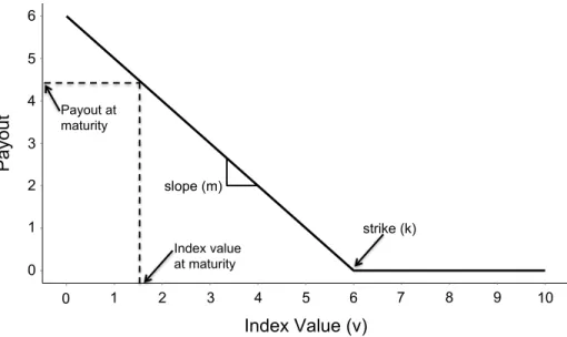
An index-based insurance contract functions by triggering a payout under conditions
specified by an agreed upon metric (or metrics) (Figure 1). This payout begins once the strike
value (k) of the index is crossed, with payouts scaled (linearly, in this example) to increase as the
absolute difference between the strike level and the index value (v) increases, as dictated by the slope (m), as described by:
!"#$%& = ( ∗ *+,[(/ − 1), 0] (1)
In Figure 1, for example, if the index value is measured at 1.5 on the maturity date of the
contract, the payout to the contract buyer would be approximately 4.4. The price the buyer pays
the seller is linked to an actuarial analysis that estimates the distribution of payouts during the
period over which the contract is in force, with the contract price then established on the basis of
a combination of expected payouts plus a loading factor.
Figure 1. Generic index-based insurance payout function
slope (m)
strike (k)
0
1 2
3
4
5 6
0 1 2 3 4 5 6 7 8 9 10
Index Value (v)
Pa
yo
ut
Index value at maturity Payout at
maturity
0 1 2 3 4 5 6
Weather derivatives often take on the form of index-based contracts, including those
based on heating or cooling degree-days (HDD/CDD), rainfall, and snowfall, all of which have
been traded on the Chicago Mercantile Exchange (Cabrera et al., 2013; CME Group, 2009). The
fact that there already exists a market for publicly traded weather-based financial hedging
instruments, particularly in the electric utility sector (HDD/CDD), and that credit rating agencies
lament the lack of a similar instrument in the water utility sector, suggests that a similar
weather-based index could be suitable in the water utility sector (CME Group, 2011; Chapman and
Breeding, 2016; Alliance for Water Efficiency, 2014; Chestnutt et al., 2014).
Several hydrologic indices are analyzed in order to characterize their correlation with
water utility operating revenue. Once the index is selected, its spatial autocorrelation is
quantified using a covariance model, which quantifies how the index is correlated with itself
across geographic locations (i.e. autocorrelation). The degree of spatial autocorrelation will
impact the probability of many insured parties receiving payouts during a single period, a
scenario of substantial interest to insurers as it impacts the size of the reserves they must
maintain, thereby increasing their costs. Generally, the spatial autocorrelation is high when two
locations are nearby to one another and decreases as the distance (i.e. spatial lag) increases. The
covariance model characterizes the relationship between decreasing spatial autocorrelation and
increasing spatial lag. The distance over which the covariance decreases to a low level (usually
set to 5% of the variance) is called the covariance spatial range, and is a critical parameter
affecting the effectiveness of risk pooling.
The spatial covariance of the index is assessed across the set of utilities for which
revenue data, often a limiting factor, is available (ideally, financial data would be available for
hydrologic index is determined, a generalized index insurance contract is developed and further
analysis is performed to assess the effectiveness of risk pooling across the set of utilities. The
total risk exhibited by the pool of contracts is then evaluated with attention to the one-year
99.5% value at risk (VaR), a measure of the risk of very high payouts in any individual period (in
this case one year), and a threshold level often used by regulators to determine reserve size
requirements for insurers (American Academy of Actuaries, 2015; IAIS, 2017). The 99.5% VaR
can be determined using historical or synthetic data in which it is the value corresponding to the
lowest 0.5% of data. For example, if a dataset with 1,000 trials was assessed, the 99.5% VaR
would be the 5th lowest value. This value would reflect the most that the company could expect
to lose, with 99.5% confidence in a one-year period.
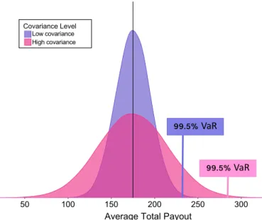
For events in which the payouts to the insured parties exhibit a long covariance range (i.e.
spatial autocorrelation over long distances), such as to homeowners in South Florida when a
hurricane strikes, the total reserves an insurer must maintain, relative to expected payouts, are
significantly greater than the reserves an insurer would need to maintain for payouts that would
occur for more independent events that exhibit very short covariance ranges and a lack of spatial
autocorrelation (e.g. automobile collisions). For events exhibiting lower spatial autocorrelation,
the distribution of aggregate payouts displays a lower variance about the expected value, leading
Figure 2. Illustrative example of the effects of covariance on VaR: When spatial autocorrelation increases (i.e. the level of independence decreases), the VaR increases
This analysis aims to explore the effects of risk pooling under conditions in which the
insured risks have differing degrees of spatial autocorrelation. The drought-related financial risks
experienced by the utilities exhibit some level of spatial autocorrelation, and consequently, so
will the payouts an insurer would make on a pool of contracts indexed to a drought metric. This
analysis makes use of a unique data set that includes coincident financial and hydrologic
information from 315 publicly operated surface water utilities spanning 68 NOAA climate
divisions across the U.S., (from Alabama, California, Florida, Georgia, Kentucky, Michigan,
North Carolina, Ohio, Oregon, South Carolina, Tennessee, Texas, Utah, Washington and
Wisconsin) all of which had at least eight years of coincident financial and hydrologic data
available between 2003 and 2012 (Figure 3).
0.000
0.005
0.010
0.015 0.020
0 50 100 150 200 250 300 350
Average Total Payout
Pro ba bi lit y Covariance Level Low Covariance High Covariance
99.5% VaR
99.5% VaR
Low covariance High covariance Covariance Level 0.000 0.005 0.010 0.015 0.020
0 50 100 150 200 250 300 350
Average Total Payout
Pro b a b ili ty Covariance Level Low Covariance High Covariance 0.000 0.005 0.010 0.015 0.020
0 50 100 150 200 250 300 350
Average Total Payout
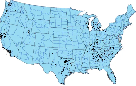
Figure 3. Locations for the 315 utilities used in this study (divisions indicate NOAA climate division boundaries)
All 315 utilities are publicly operated water utilities, meaning that they are non-profit
entities led by elected and appointed public officials. Because of this, raising rates on short
notice and/or maintaining large reserves of unallocated funds, can be very difficult (Alliance for
Water Efficiency, 2014). This work focuses exclusively on utilities drawing on surface water
since these systems feel a more immediate and direct financial impact from hydrologic
variability.
2.2.1 Identifying an effective index
To create an index-based financial contract, it is necessary to characterize the relationship
between hydrologic behavior and the related financial risk. Candidate hydrologic indices could
include precipitation, streamflow, reservoir storage, and drought indices (e.g. Palmer drought
period. An effective index should be transparent, publicly available, not easily manipulated, and
strongly correlated with the financial metric(s) of interest. Most systems dependent on surface
water include some form of reservoir storage, so low reservoir levels may be an obvious signal
of drought (and the need to conserve water). However, reservoir levels can be impacted by the
actions of the utilities themselves, making them open to concerns over manipulation or moral
hazard and thus less suitable. Other candidate indices, such as precipitation, streamflow, and
drought indices, are transparent, involve publicly available data and act as reasonable proxies for
drought. The question then becomes how well these indices correlate with utility financial risk.
In this work, financial risk is measured in terms of the reductions in utility operating revenue,
often a result of reduced water sales that in many cases can be linked to drought-related
restrictions on water use. Since short-term utility costs are mostly fixed, large and unexpected
reductions in operating revenue can introduce a substantial financial risk to water systems
(Hughes and Leurig, 2013; Hanemann, 1997; Omlstead and Stavins, 2009).
The degree to which the index and financial risk are uncorrelated is typically termed
“basis risk”; If basis risk is high, then payouts will not match up well with financial losses and
vice versa, leaving the insured party (i.e. the water utility) with more risk exposure than they
expect, as well as the potential for payouts when no (or few) losses occur. The insurer, on the
other hand, will make decisions regarding contract prices and payouts based upon the behavior
of the index itself, which is often well characterized and so is less concerned with the timing of
payouts to individual utilities as long as the total payouts are in line with the insurer’s estimates.
Earlier research focused on very detailed indices constructed to suit the circumstances of
individual water utilities (Zeff and Characklis, 2013; Zeff et al., 2014; Zeff et al., 2016). These
be difficult to implement broadly, given the data required to evaluate hydrologic conditions at
each utility. One objective of this work is to explore the performance of alternative indices which
will be more broadly applicable, even if they exhibit somewhat higher basis risk than an index
tailored to each individual utility.
2.2.2 Hydrologic indices and correlation with operating revenue
Precipitation, streamflow, and the Palmer Hydrologic Drought Index (PHDI) were tested
to determine the strength of their correlation with operating revenues across the set of utilities
considered. Implicit in this analysis is the assumption that nearly all utilities respond to drought
by imposing water use restrictions. While each utility’s unique pricing scheme (e.g. fraction of
fixed vs. volumetric charges, seasonal rates, end-use tariffs, etc.) will influence each utility’s
relationship between drought and reduced revenues, a general link between the two has been
well documented (Chapman and Breeding, 2016; Chesnutt et al., 2014; Eskaf et al., 2014;
Alliance for Water Efficiency, 2014; Hughes and Leurig, 2013). Each of the three hydrologic
variables investigated has datasets of historic observations publicly available from either the
National Oceanic and Atmospheric Administration (NOAA) (NOAA Climatic Data Center,
2017) or the United States Geological Survey (USGS) (USGS Water Webserver Team, 2016).
Precipitation and streamflow data are available on a daily timestep while drought index values
are available monthly. Utility revenue data, at least over the spatial and temporal scales required,
were obtained from Moody’s Water and Sewer Municipal Financial Ratio Analysis (Moody’s)
(Moody’s Analytics, 2017), but were only available at an annual timestep. The coarser
discretization of the revenue data led to assessing correlations between candidate indices and
for individual utilities presents some challenges, but for the purposes of this work, an assumption
is made that all revenue totals correspond to the calendar year (January to December).
While precipitation and streamflow measurements are straightforward, the PHDI assesses
deviations in moisture from normal conditions based on a water balance equation that considers
precipitation, evapotranspiration, soil moisture loss, recharge, and runoff in order to determine
when droughts begin and end (Palmer, 1965). These PHDI values are normalized on a scale from
-12 (indicating severe drought) to +12 (indicating extreme wetness) in order to compare drought
levels across the United States. PHDI monthly data were obtained from NOAA (NOAA Climatic
Data Center, 2017) at each of the 68 climate divisions in which the studied utilities were located
over the 120-year period of record from January 1896 to December 2015. Each utility was
assigned the PHDI value for the climate division in which it resided. The average PHDI for each
year (January to December) was determined for each water utility. Since PHDI is based on a
normalized scale, these values were used. It should be noted that utility revenues can also decline
with extreme wetness, as customers may not purchase as much water for outdoor use (Tiger et
al., 2014; Hughes et al., 2014). As revenue reductions during wet weather are not the focus of the
current analysis, average annual PHDI values greater than +3 (indicating very wet conditions)
were removed, as these higher PHDI values would otherwise confound the correlation between
PHDI and reduced revenue (Table 1). The financial effects of very wet weather may be
Table 1. Data characteristics for each tested index
Index Location Timestep Adjustment
PHDI Climate division Average annual (from monthly)
Removed all PHDI values greater than 3
Precipitation Nearest
precipitation gauge
Average annual (from monthly)
Removed all values above 1 standard deviation
Streamflow Nearest upstream streamflow gauge
Average annual (from monthly)
Removed all values above 1 standard deviation
Total monthly precipitation data were retrieved from NOAA’s Annual Climatological
Summary (NOAA Climatic Data Center, 2017). Additionally, a list of all precipitation gauge
sites and their locations were obtained and then mapped with the utility locations to determine
the three nearest gauges to each utility. Three gauges were used to smooth any inconsistencies in
data from a single gauge. The three nearest sites were determined via ArcGIS10.1, and each
assessed to ensure that monthly data were available from 2003-2012 (the period over which
revenue data were also available). Average precipitation in each year was determined for each
precipitation gauge nearest to each water utility (Table 1).
Streamflow data were obtained from USGS in the form of average daily mean
streamflow discharge (USGS Code 00060) over a monthly period (USGS Water Webserver
Team, 2016). The nearest upstream sites were determined via ArcGIS10.1 through mapping all
the streamflow sites to find the nearest gauges and then ensuring they were upstream based on
USGS streamflow station codes, which are numbered such that on any tributary, upstream site
numbers are lower than those downstream (USGS Annual Water Data Report, 2017). The
nearest upstream gauge with streamflow data from 2003-2012 was used. Average daily mean
streamflow for each year (January to December) was determined from monthly values. As with
dry conditions (excluding wet conditions), so streamflow values greater than 1 standard
deviation above the mean were removed for this analysis (Table 1).
Revenue time series data are detrended to account for increases in population and
aggregate demand, assuming linear growth. For each utility, detrended revenues are analyzed
with respect to their correlation with the candidate indices. Coincident time series of detrended
revenues and candidate indices are then jointly assessed in terms of Pearson correlation values to
determine the strength of the correlation between them.
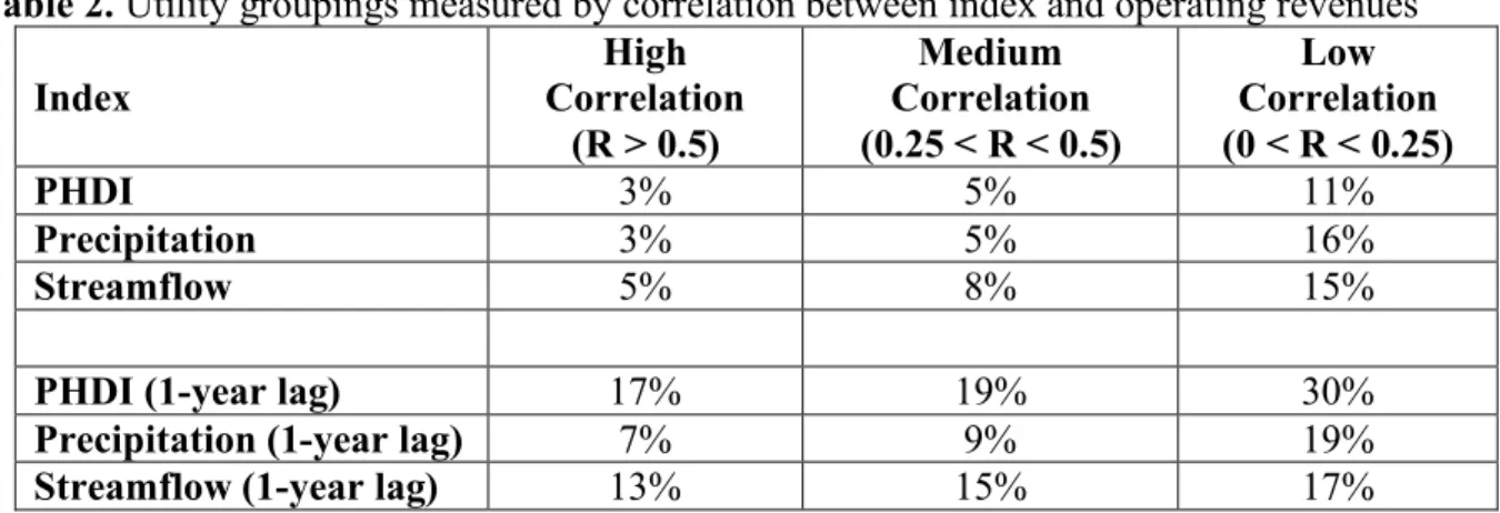
The correlation between operating revenues and hydrologic indices evaluated in the same
year are somewhat low (Table 2). However, there can often be a significant lag between the time when conservation measures are imposed and when revenues decline, so correlations between utility revenues and hydrologic indices are also evaluated with the index value lagged by 1 year (Table 2). This lagged correlation is substantially higher, likely due to many factors, including utility billing practices and the timing of conservation measures. While most utilities bill their customers monthly, very few read meters that often. Rather, most read them on a bimonthly or quarterly basis, using the previous year’s consumption for the same period (or an average of previous years) as a proxy for the unmeasured period, which is used for billing until the meter is read somewhat later, at which time the bill is reconciled with actual usage. In addition, the low point for most surface water supplies (i.e., when conservation measures are imposed) comes in the late summer/early fall, following the primary irrigation season, a time which also coincides with the end of the fiscal year (30 September). These two factors, or in many cases the
Table 2. Utility groupings measured by correlation between index and operating revenues
Index
High Correlation
(R > 0.5)
Medium Correlation (0.25 < R < 0.5)
Low Correlation (0 < R < 0.25)
PHDI 3% 5% 11%
Precipitation 3% 5% 16%
Streamflow 5% 8% 15%
PHDI (1-year lag) 17% 19% 30%
Precipitation (1-year lag) 7% 9% 19%
Streamflow (1-year lag) 13% 15% 17%
Note: percentages do not sum to 100% as some utilities exhibited negative correlation between the index and revenues
When assessing the performance of the index insurance contracts, water utilities were
separated into three different groups, indicating different levels of correlation between the
hydrologic variable and operating revenue, with the strength of the correlation corresponding
roughly to the utility’s drought-related financial risk. In this work, a distinction is made between
utilities in which Pearson correlation between the index and revenues is greater than 0.5 (high
risk), between 0.25 and 0.5 (medium risk), and less than 0.25 (low risk). These groupings also
indicate the level of basis risk inherent in an insurance contract based on a given index, with high
correlations (>0.5) suggesting a more effective index on which a contract might be based. Thus,
those utilities with a high correlation between revenues and the index will be both more at risk of
drought related losses, and more likely to find the index-based contracts effective in insuring
against this risk.
Precipitation was poorly correlated with utility revenues, both with and without a
one-year lag, and was discarded as an ineffective index. The PHDI index with a one-one-year lag was
most strongly linked with declining utility revenues, with 17% exhibiting a correlation greater
than 0.5. However, the spatial resolution of PHDI is less highly resolved than that of streamflow.
values, publicly available through NOAA, are available at a climate division level (see Figure 1)
while streamflow values are available at a finer scale, closer to the exact location of each water
utility. Since streamflow had similarly strong correlations to water utility revenues, and is also
transparent and not easily manipulated, and seemed likely to also be intuitive to both insurers and
utilities (a potentially important marketing consideration), financial contracts based on both
PHDI and streamflow are developed in this work.
Findings indicate that 45% of the utilities analyzed have revenues that exhibit some level
of correlation (greater than zero) with annual average daily streamflow lagged by one year and
66% of utilities have revenues that correlate to some level with a one year lag in annual average
PHDI. For streamflow and PHDI, 13% and 17% of utilities, respectively, have a correlation
coefficient greater than 0.5, indicating high financial vulnerability to drought, as well as the
potential for relatively effective insurance via an index-based contract. These correlation levels
are consistent with levels exhibited by many hedging instruments currently in use. Publicly
traded and broadly employed weather-based hedging contracts often have R2 values ranging
from 0.9 to 0.2 (Manfredo and Richards, 2005; Norton et al., 2010). While contracts based on
streamflow and PHDI may not be suitable for every utility, this analysis suggests that they have
the potential to be useful to a significant fraction of the 15,000 surface water dependent utilities
in the United States.
2.2.3 Sharing risk through spatial diversification
From the perspective of the insurer, there is less concern over the level of basis risk for an
indexed product, except as this might act to reduce the attractiveness of the contract to potential
linked to the index) and the size of the reserves that must be maintained in order to meet
regulatory standards designed to ensure solvency. To the insurer, the effectiveness of risk
pooling is important, and is integrally linked to the degree of independence of the insured risks,
which in this case is directly related to the degree of spatial autocorrelation associated with the
index.
While the specific levels of covariance in the PHDI and streamflow indices between each
pair of insured locations (i.e. insured utilities) must be understood in order to assess the impacts
of risk pooling (see next section), a general assessment of spatial covariance provides some
broader insights. Therefore, a spatial covariance model was developed for: (a) the 143
streamflow gauges and (b) the 245 PHDI climate division centroids, with these representing the
hydrologic conditions for the subset of utilities with index/revenue correlation values greater
than zero. Tobler’s first law of geography, that near things are more related than distant things,
suggests that as distance increases, covariance should decrease. This analysis indicates that
covariance in streamflow values decreases exponentially as a function of distance with
covariance nearing zero when there is approximately 1,000 kilometers between streamflow
gauges, with similar findings for PHDI (Figure 4). Given the spatial scale considered here (the
entire U.S.), these results suggest that there should be significant benefits from pooling the risks
Figure 4. Covariance of streamflow (top) and PHDI (bottom) values corresponding to 143 (streamflow) and 245 (PHDI) utilities that exhibit some correlation (>0) between the index and revenues;
Note that this spatial covariance model does not suggest that each utility must be 1,000 km away from another in order to experience independent conditions, but rather that this is the
farthest distance between any two utilities in the analyzed set to have a covariance near zero.It is
also important to note that risk pooling can be effective even if some degree of spatial
autocorrelation exists between the exposed parties, with the impact of risk pooling related to the
rate at which covariance decays with distance (i.e. the slope in Figure 4). A similar situation
exists when an investor limits her risk by assembling a portfolio of assets with some low level of
correlation (Markowitz, 1991). The actual degree of effectiveness, in this case, can only be
assessed by evaluating the covariance between each pair of utilities in the pool, as will be done
later in this analysis. The critical feature, of course, is that as covariance decreases, the variance
Spatial Lag (100 km)
Cov
aria
nc
e
0 5 10 15 20 25
-0.2 0 0.2 0.4 0.6 0.8 1.0
Spatial Lag (100 km)
Cov
aria
nc
e
0 5 10 15 20 25
-1 0 1 2 3 4 5
Streamflow
about the mean in the distribution of aggregate payouts will be reduced, lowering the size of the
reserves that an insurer must maintain.
2.2.4 Determining the effects of risk pooling
The remainder of this analysis focuses on the set of 143 utilities that exhibit a positive
correlation between the streamflow index and revenues, and the set of 245 utilities that exhibit a
positive correlation between the PHDI index and revenues. This work provides an opportunity to
explore the effectiveness of two different index contracts on the financial risk of the utilities that
are exposed to drought. Since the utilities that compose these two groups of index contracts are
not the same and the correlations between the index and revenues differ for each index, the
results between them are not directly comparable in absolute terms. Rather, it is the relative
difference between risk pooling strategies and those based on self-insurance or risk shifting
approaches, compared across both the PHDI and streamflow indices, that provides insight into
the effectiveness of risk pooling.
Three scenarios are compared to assess the advantages of risk pooling: self-insurance,
risk shifting, and risk pooling. These scenarios can be thought of as representing situations in
which: each utility elects to set aside sufficient reserves to self-insure (self-insurance), each
utility signs a separate contract with a different insurer (risk shifting), or all the utilities
collectively pool their risks and are managed by one insurer (risk pooling). Whether the risks are
pooled or managed independently (via self-insurance or risk-shifting), some level of reserves
will need to be maintained to compensate for drought-induced losses. The size of these reserves,
one for pooled risks and the other an aggregate of individual reserves (maintained by the utilities
maintaining that reserve. To make the scenarios comparable, the size of these reserves will be
described in terms of the value at risk (VaR), set at the 99.5% level.
In order to evaluate the impacts of risk pooling, several assumptions must be made to
develop contracts and set levels of coverage. To do this, the utilities are separated into three
groups based on different correlation levels (high, medium, and low) between the hydrologic
index (streamflow or PHDI) and operating revenue. This also allows for some distinction
between the amounts of coverage assumed to be purchased by each group, with the thought that
those experiencing a high correlation between the index and revenues (i.e. those most at risk)
would likely purchase more coverage.
The PHDI and streamflow values at which utilities would most likely desire some level
of financial risk mitigation for drought events were determined based on standardized values
indicating severe drought. For the PHDI index, a value below -3 is considered to represent
“severe drought” (Palmer, 1965), so it was used as the strike value for the PHDI-based contract.
For streamflow, any normalized value falling more than 1 standard deviation below the mean is
considered severe drought. One standard deviation below the mean covers the lowest 16% of
streamflow events which is comparable to the 18% of events classified as moderate to extreme
drought based upon PHDI (Alley, 1984). As PHDI is already normalized for each climate
division, the same PHDI strike value (-3) is used for each utility’s contract. In the case of
streamflow-based contracts, each utility’s contract has its strike set at one standard deviation
below the mean, but this translates to a different streamflow level for each. A general depiction