MITIGATING REAL-VIRTUAL DISPARITIES IN ILLUMINATION AND DYNAMIC POSITION IN OPTICAL SEE-THROUGH AUGMENTED REALITY
Alex Blate
A dissertation submitted to the faculty at the University of North Carolina at Chapel Hill in partial fulfillment of the requirements for the degree of Doctor of Philosophy in Computer Science.
Chapel Hill 2019
Approved By: Henry Fuchs Mary C. Whitton
Montek Singh Gregory F. Welch
© 2019 Alex Blate
ABSTRACT
Alex Blate: Mitigating Real-Virtual Disparities in Illumination and Dynamic Position in Optical See-Through Augmented Reality
(Under the direction of Henry Fuchs and Mary C. Whitton)
A user of an optical see-through (OST) augmented reality (AR) display sees virtual objects optically-combined with and referenced to the real world. Real-virtual disparities occur when the
appearance or behavior of a virtual object differs from the user’s expectations for real-world objects. This dissertation addresses the mitigation of real-virtual disparities in illumination (appearance) and dynamic position (behavior).
Disparities in illumination occur when a virtual object’s brightness does not match its real-world surroundings. We present an illumination method for binary frame-based displays – Dynamic Binary Frame Illumination (DBI) – wherein each binary frame can be illuminated at any intensity and color within the illuminator’s dynamic range. We demonstrate a DBI-illuminated, 16 bit-per-color RGB OST AR display with 115 dB of luminous dynamic range and motion-to-photon latency of about 110 μs. Using our prototype position-sensitive light sensor, this display is able to adjust virtual objects’ intensities to match the real-world for most lighting conditions.
ACKNOWLEDGEMENTS
I must begin by thanking my wife, Yani Blate, for her extraordinary support – without which my Doctoral studies would not have been possible. When we moved to Chapel Hill, Yani was six months’ pregnant with our daughter, Natalie, whose love, affection, and amazing development have helped sustain my spirits and perseverance over the past five years. I also thank my mother, Toni Lee Blate, for her support and encouragement.
I would like to thank my advisors, Henry Fuchs and Mary C. Whitton, for their guidance, tutelage, and patience.
Henry has a gift for discovering and spreading excitement about aspects of what might otherwise be less accessible technical work; his imagination is inspiring and elevates the work of those around him.
I learned to write from my late father, Professor Sam Blate (UNC class of 1965), who created the Creative Writing curriculum at Montgomery College (Rockville, MD). Over the past two years, Mary has taught me how to write de novo – how to write in the manner of a technical scholar; she helped me find a new voice. I thank Mary for being tough on me in all the right ways – occasionally to the point of our mutual exasperation – and for the enormous amount of time she has invested in me.
I thank the other members of my committee, Montek Singh, Greg Welch, and Turner Whitted, each of whom, in his own way, has indelibly advanced the way I think, write, and communicate. I also thank Andrei State who, for all intents and purposes, has essentially been a member of my committee and whose late-night linguistic prowess helped several papers over the finish line.
I would like to thank my other collaborators: Kishore Rathinavel, Hanpeg Wang, and Anselmo Lastra. I am grateful to Praneeth Chakravarthula, David Dunn, Kurtis Keller, and Gary Bishop for their technical assistance and moral support. I thank Jim Mahaney for providing engineering and logistical assistance throughout this process and for trusting me to use the Department’s machine shop and teaching me to use it efficiently.
I thank Missy Wood, Jodie Turnbull, and Michael Fern for their administrative assistance, including their help in maintaining my TA/RA funding while transitioning advisors and thesis topics.
I thank Jim Anderson, Kevin Jeffay, and Jan Prins for enabling my readmission to the PhD program.
I am grateful for the funding enabled and/or provided by Fabian Monrose, Prasun Dewan, Mitre Corporation, and the National Science Foundation (NSF).
Tabatha Peck (PhD 2010), whom I met at IEEE VR 2016, gave me the single most important piece of advice about my graduate studies: do whatever you can to get Mary Whitton on your committee. Thank you, Tabatha.
I thank Don Stanat (Professor Emeritus) for teaching me, among other things, how to think about programming, and for his mentorship and friendship over the past 22 years. I thank my former manager, Eric Nielsen, PhD, for his mentorship, friendship, and for encouraging me to pursue a PhD. I am forever indebted to Nancy Metz, my eleventh-grade mathematics teacher, for sparking my love of mathematics and thereby changing the trajectory of my education.
I have had the privilege of teaching four undergraduate classes; I am grateful to the Department, the University, and the Summer School for this opportunity. Moreover, I am grateful to my students and for how much I learned from them.
TABLE OF CONTENTS
LIST OF TABLES ... xii
LIST OF FIGURES ... xiii
LIST OF ABBREVIATIONS ... xv
LIST OF SYMBOLS ... xviii
CHAPTER 1: INTRODUCTION ... 1
1.1 Thesis Statement ... 5
1.2 Supporting Contributions, Evidence, and Results ... 6
1.2.1 Illumination ... 6
1.2.2 Dynamic Position (Tracking Instrument) ... 9
1.3 Organization ... 14
CHAPTER 2: ON MOTION TO PHOTON LATENCY ... 15
2.1 Motion-to-Photon Latency: Definitions ... 18
2.2 Latency in Augmented and Virtual Reality: Background ... 20
2.3 Mitigating Display Latency Sources ... 22
2.4 Perceiving a Stationary World When One Moves ... 24
2.5 Perception of Latency in Optical See-Through Augmented Reality ... 25
CHAPTER 3: MITIGATING DISPARITIES IN ILLUMINATION ... 27
3.1 Introduction ... 28
3.2 Related Work and Background ... 33
3.2.1 High Dynamic Range Displays ... 33
3.2.3 The Human Element ... 35
3.2.4 Binary Frame Displays and Digital Micromirror Device-Based Projectors ... 35
3.3 Dynamic Binary Frame Illumination (DBI) Illuminator Design and Implementation ... 38
3.3.1 Dynamic Binary Frame Illumination (DBI)... 42
3.3.2 DBI Illuminator: A Priori Requirements ... 45
3.3.3 Illuminator: High-Level Design ... 50
3.3.4 Current Source Implementation ... 53
3.3.5 LED Pre-Biasing and Dark Level Calibration ... 55
3.3.6 Control Signaling and Timing ... 58
3.4 Validation ... 59
3.4.1 Dynamic Range ... 59
3.4.2 Temporal Characteristics ... 68
3.4.3 Application 1: High Dynamic Range, Scene-Adaptive, Low-Latency Optical See-Through Augmented Reality Display ... 72
3.4.4 Application 2: Full-Color Volumetric Near-Eye Display ... 85
3.5 Future Work ... 86
3.5.1 Dynamic Range ... 86
3.5.2 Self-calibration, thermal compensation ... 87
3.5.3 Application: Video Projectors ... 87
3.5.4 Power Efficiency ... 88
3.5.5 Lasers ... 89
3.5.6 Position-Sensitive Light Sensors ... 90
3.6 Conclusion ... 90
CHAPTER 4: MITIGATING DISPARITIES IN DYNAMIC POSITION ... 92
4.2 Related Work ... 97
4.3 Tracking Instrument ... 100
4.3.1 Nominal Performance Requirements: Informed Engineering Estimates ... 100
4.3.2 Overview and Performance Summary ... 106
4.3.3 Design, Architecture, and Implementation ... 111
4.3.4 Latency and Timing Analysis ... 125
4.3.5 Spatial Resolution and Tracking Volume ... 127
4.3.6 Tracking Instrument: Conclusion ... 130
4.4 Real-Virtual Displacement and Latency Measurement Technique ... 130
4.4.1 Dynamic Tracking Error ... 131
4.4.2 Measurement Principle of Operation ... 133
4.4.3 Video Data Post-Processing ... 138
4.5 Experimental Results ... 139
4.5.1 Experimental Setup ... 139
4.5.2 Experiments ... 140
4.5.3 Results ... 143
4.6 Future Work ... 146
4.6.1 Extended Tracking Volume ... 146
4.6.2 Perceptual Studies and Integration with Low-Latency OST AR HMDs ... 149
4.7 Conclusion ... 150
CHAPTER 5: SUMMARY AND CONCLUSIONS ... 151
5.1 Disparities in Illumination ... 152
5.2 Disparities in Position ... 152
LIST OF TABLES
Table 1: Efficiency of PTM (pulse train modulation) and dynamic binary frame
illumination (DBI) as a function of dynamic range. ... 41 Table 2: Illuminator dynamic range ... 62 Table 3: Maximum MTPL and pose sample frequency (FS) versus rotational rate
LIST OF FIGURES
Figure 1: Notional tracker (outside-looking-in paradigm). ... 16
Figure 2: Motion-to-photon latency: schematic definition. ... 17
Figure 3: Dynamic range of human vision. ... 30
Figure 4: Digital Micromirror Device (DMD): Example of device and micrograph of mirror array. ... 31
Figure 5: Optical signal path of a color wheel-based DMD projector. ... 32
Figure 6: Optical signal path of LED-illuminated DMD projector. ... 32
Figure 7: OST AR HMD apparatus of (Lincoln, Blate, et al. 2017). ... 37
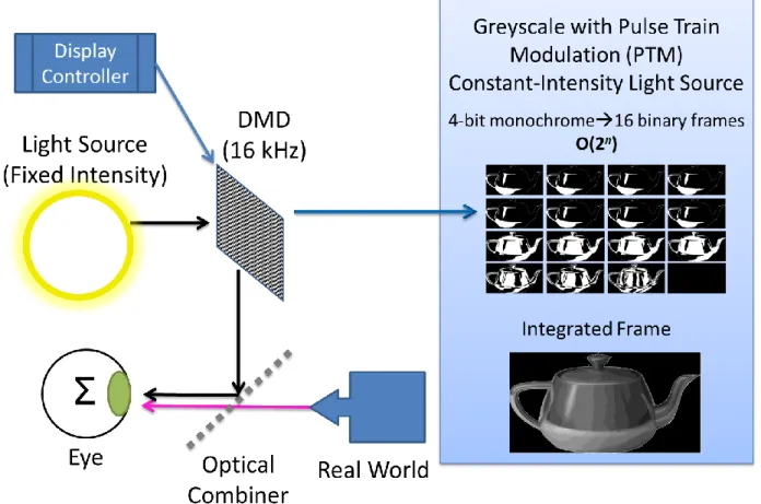
Figure 8: Traditional DMD-based OST AR display: Notional block diagram. ... 39
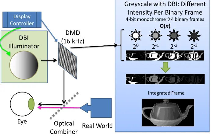
Figure 9: DBI-illuminated DMD-based OST AR display: Notional block diagram. ... 40
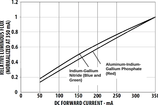
Figure 10: Luminous flux (normalized) vs. forward current for ASMT-MT00 RGB LED. ... 48
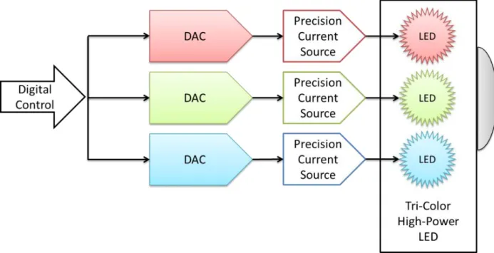
Figure 11: Illuminator block diagram. ... 49
Figure 12: Avago™ ASMT-MT00 RGB LED ... 49
Figure 13: Current source simplified schematic. ... 51
Figure 14: DBI illuminator PCB/implementation. ... 52
Figure 15: Illuminator analog and digital timing (not to scale). ... 57
Figure 16: Illuminator full-scale pulse (control signal and analog response). ... 66
Figure 17: Illuminator full-scale transition: zoomed-in view of rising edges. ... 67
Figure 18: Position-sensitive light sensor prototype: principle of operation. ... 74
Figure 19: Cut-away of a prototype baffle for position-sensitive light sensor. ... 75
Figure 20: Position-sensitive light sensor circuit board. ... 75
Figure 21: HDR OST AR display demonstration. ... 79
Figure 23: Volumetric near-eye display depth decomposition. ... 83
Figure 24: Volumetric near-eye display: view through display. ... 84
Figure 25: Tracker axes with respect to user ... 104
Figure 26: Tracker axes relative to sensors. ... 105
Figure 27: Duo-lateral photodiode structure. ... 107
Figure 28: Tracking instrument block diagram. ... 108
Figure 29: Tracking instrument physical overview. ... 109
Figure 30: HMD mock-up. ... 110
Figure 31: Pose acquisition and calculation: notional algorithm ... 116
Figure 32: Tracker timing diagram. ... 124
Figure 33: Latency measurement experimental setup. ... 134
Figure 34: Quadrature velocity encoding example. ... 135
Figure 35: Latency analysis (no added latency). ... 141
LIST OF ABBREVIATIONS
2D Two-Dimensional
3D Three-Dimensional
6D Six-Dimensional
6-DOF Six-Degree-of-Freedom
A Amperes (SI unit of electrical current) ADC Analog-to-Digital Converter
API Application Programming Interface
AR Augmented Reality
BJT Bipolar Junction Transistor
bpp Bits per pixel
BSLM Binary Frame Spatial Light Modulator cd Candella (SI unit for luminous intensity) CLK Clock (digital signalling)
CLR Clear (digital signalling) COTS Commercial Off-The-Shelf CPU Central Processing Unit
CRT Cathode Ray Tube (picture tube) CS Chip Select (digital signaling) DAC Digital-to-Analog Converter
dB Decibel (field/amplitude scale unless otherwise specified) DBI Dynamic Binary Frame Illumination
dBmV Decibels, referenced to 1 mV
DC Direct Current
DMA Direct Memory Access
DOF Degree(s of Freedom FIFO First-in, First-out
FOV Field-of-View
FPGA Field-Programmable Gate Array GPU Graphics Processing Unit
GSPS Giga-Samples per Second (one billion samples per second)
HDR High Dynamic Range
HMD Head-Mounted Display
IR Infrared
IRQ Interrupt Request
LCD Liquid Crystal Display LCoS Liquid Crystal on Silicon
LED Light Emitting Diode
LEPD Lateral-Effect Photodiode LSB Least-Significant Bit
lx Lux (SI derived unit of illuminance)
MOSFET Metal Oxide Semiconductor Field Effect Transistor MOSI Master Out, Slave In (digital signaling)
MSB Most-Significant Bit
MSPS Mega-Samples per Second (1 million samples per second)
MTPL Motion-to-Pose Latency
OLED Organic Light Emitting Diode
OST Optical See-Through
PCB Printed Circuit Board
PDM Pulse Density Modulation
PR-PDM Pseudo-Random Pulse Density Modulation
PWM Pulse Width Modulation
RAM Random-Access Memory
RGB Red, Green, and Blue
RMS Root Mean Square
SAR Sequential Approximation Register
SI International System of Units (Système International)
SLM Spatial Light Modulator
SNR Signal-to-Noise Ratio
SoC System-on-Chip
USB Universal Serial Bus
V Volts (SI derived unit of electrical potential)
VDC Volts, Direct Current
VR Virtual Reality
LIST OF SYMBOLS
∝ Proportional to (binary operator)
ErrA Dynamic tracking error with respect to axis A
ErrRVA Real-virtual displacement with respect to axis A
FS Pose sample rate
LDISP Display latency (see section 2.1)
LTRACK Tracking latency (MTPL-TS)
MTPL Motion-to-pose latency (see section 2.1) N(VA,t) Pose uncertainty
Pi Pose output i (for integer i)
t Time
TS Pose sample period
u, v Sensor coordinates
VA Pose velocity with respect to axis A
X, Y, Z Cartesian coordinate axes
CHAPTER 1: INTRODUCTION
Users of optical see-through (OST) augmented reality (AR) head-mounted displays (HMDs) see virtual objects optically-combined with and referenced to their views of the real world. Each of us has a well-developed set of expectations for the appearance and behavior of real-world objects. When an element of a scene, e.g., a virtual object, fails to meet either or both of those expectations, the real-virtual disparity is unavoidably obvious – potentially to the point of the user’s distraction or distress. Within limits, users can adapt to a uniformly different environment, such as that experienced in virtual reality (VR), where one’s view is entirely under the control of the VR system. In contrast, in OST AR, a direct view of the real world is constantly present and virtual objects will unavoidably be perceived in relation to our expectations for real-world objects and our present experience of our real-world surroundings. Significantly more-stringent visual and temporal performance is required in OST AR systems in order to minimize real-virtual disparities, i.e., for virtual objects to satisfy the expectations we have for real objects. This dissertation focuses on and introduces techniques that make significant steps towards mitigating two specific real-virtual disparities, each discussed in turn, below: disparities in illumination (the luminosity1 or brightness of virtual objects) and in disparities dynamic position (the positions of virtual objects relative to the real world when the user is moving).
A real-virtual disparity in illumination can arise due to mismatches between the luminosity (brightness) of virtual objects and their real-world surroundings. The luminosity in a typical real-world scene may vary over five to six orders-of-magnitude, e.g., from dark shadows to bright sunlight. To provide real-virtual consistency in luminosity: the OST AR system must have knowledge about the
1 Unless otherwise specified, the word “luminosity” is used according to its common meaning, i.e., a relative
luminosity of the regions of the scene in which virtual objects are positioned; and the display’s range of luminosities – it’s dynamic range – must be commensurate to that of the scene. A virtual object’s
luminosity may need to be adjusted based on its location in the scene such that its luminosity is consistent with the scene luminosity at the object’s location. This process is called scene-adaptive illumination (Lincoln, Blate, et al. 2017). Whatever approach is taken to mitigate disparities in illumination must not introduce new real-virtual disparities, such as those caused by display latency. For example, display latency is well-known to cause real-virtual registration errors (Holloway 1997), so, ideally, our approach must not increase display latency.
In the first major part of this dissertation, we propose and demonstrate a new method of
illumination for displays based on binary frame spatial light modulators (BSLMs). BSLM-based displays output 1-bit monochrome binary frames at a high binary frame rate (on the order of 4-32 kHz); these high binary frame rates have been leveraged to build low-latency OST AR displays (Lincoln, Blate, et al. 2016). Due to persistence of vision, humans perceive the time-domain integration of a set of binary frames as a continuous-tone image – an integrated frame. For a given binary frame rate, the integrated frame rate is the binary frame rate divided by the number of binary frames per integrated frame; the reciprocal of the integrated frame rate is the integrated frame time (or period).
To output n-bit greyscale images, conventional BSLM displays, which use fixed-intensity light sources, require O(2𝑛) binary frames per integrated frame – i.e., the number of binary frames per integrated frame exponential in bits per pixel. Our method, which we call Dynamic Binary Frame Illumination (DBI), uses a variable-intensity light source and allows the luminosity and color of illumination of each binary frame to be chosen arbitrarily from the illuminator’s dynamic range. Using DBI, the number of binary frames per integrated frame is O(𝑛) – i.e., linear in bits-per-pixel. Said more simply, DBI uses the BSLM more efficiently vis-à-vis the number of binary frames required for each integrated frame2. We wish to extend the display’s luminous dynamic range – i.e., increase n. DBI’s
efficiency allows us to extend the display’s dynamic range while not increasing, but in fact reducing the display’s integrated frame time, and thus reducing display latency3
.
To implement scene-adaptive illumination, the display controller requires information about the luminosity of areas of the real-world scene occupied by virtual objects. Given this positional luminosity information, the display controller can adjust virtual objects’ luminosities to match the real world. To this end, we present the principle of position-sensitive light sensing and demonstrate a prototype
implementation of a high dynamic range position-sensitive light sensor. Note that this dissertation does not address how the display performs or implements scene-adaptive illumination. Rather, we identify the need for and demonstrate a prototype implementation of a position-sensitive light sensor. The output of this sensor is used by a display, such as that reported by Lincoln (2017), to perform such adaptation
In summary, real-virtual disparities in illumination are mitigated by providing the display controller with a high dynamic range output device (enabled by DBI) and input from a position-sensitive light sensor. Given an output device whose luminous dynamic range is commensurate to the real-world scene and positional scene luminosity information, the display controller adjusts virtual objects’ luminosities to match the real world, i.e., scene-adaptive illumination.
The dynamic position of a virtual object is the virtual object’s location during user head movement. A disparity in dynamic position is a displacement, as seen by the user, between the virtual object’s intended real-world location and where the virtual object actually appears on the display; we call this displacement a dynamic real-virtual displacement. Users often perceive dynamic real-virtual
displacements as discontinuous and unintended movement of virtual objects with respect to their intended real world positions. More generally, dynamic real-virtual displacement creates the appearance of
movement of virtual objects whose locations are intended to be fixed. For a given change in user pose
3
over time, which we call pose velocity4, the magnitude of real-virtual displacement is proportional to the latency between: a) a movement occurring (stimulus) and b) the changes to the display’s output reflecting the user’s new pose (response). This latency is known as the system’s motion-to-photon latency5
. Head tracking latency is one component of motion-to-photon latency. Because virtual objects in OST AR are always seen with respect to the real world, head tracking requirements – and latency requirements in general – in OST AR are more stringent than those in VR, where the entire scene is virtual (Bishop, et al. 1994). Mitigating real-virtual displacements in OST AR requires head tracking with higher sample rates, lower latency, and greater precision than previously demonstrated (the beginning of section 4.3 justifies this statement quantitatively).
In the second major part of this dissertation, we present the design, implementation, and
validation of an optical head tracking instrument with the lowest latency (28 μs) and highest sample rate (50 kHz) of any previously-reported non-mechanical tracker(s). This instrument is intended for use in developing and studying low-latency OST AR displays and for psychophysical research, such as determining perceptual thresholds for motion-to-photon latency. To verify and quantify our tracking instrument’s dynamic temporal and spatial performance, we developed and demonstrate a measurement apparatus and technique for directly and precisely measuring tracking latency, real-virtual displacement, and tracking repeatability. The technique and apparatus use inexpensive, readily-available components and generalizes for use with other trackers or other applications, such as measuring the response time of a motion sensor. We use our technique and apparatus to measure our tracking instrument’s motion-to-pose latency (28 μs) and assess its repeatability (under one arcminute6, which is below human static visual acuity) and dynamic tracking error (under 2 arcminutes at over 500°/s, which is below human dynamic visual acuity (Regan and Miller 2017)).
4 Pose velocity is the union of translational velocity and rotational velocity.
5 The term “motion-to-photon latency”, used in this dissertation, is defined in section 2.1. 6
1.1
Thesis Statement
Disparities in illumination and dynamic position between the real-world and virtual content in Optical See-Through Augmented Reality (OST AR) can be mitigated:
1) Illumination
a) Dynamic Binary Frame Illumination (DBI) extends the luminous dynamic range and reduces the display latency of binary frame spatial light modulator-based OST AR displays.
b) With DBI and position-sensitive light sensing, OST AR displays can mitigate real-virtual disparities in illumination by adjusting the luminosity of virtual objects to match their real-world locations.
2) Dynamic Position
a) It is possible to build an instrument for tracking head pose in six-degrees-of-freedom whose dynamic tracking error is under 2 arcminutes at rotational velocities of over 500°/s – such that discrepancies in dynamic position are below human dynamic visual acuity.
1.2
Supporting Contributions, Evidence, and Results
The claims of our thesis statement are supported by the research, implementations, experimental evidence, and performance analyses presented in this dissertation, as summarized below:
1.2.1
Illumination
Claim (1a): “Dynamic Binary Frame Illumination (DBI) extends the luminous dynamic range and reduces the display latency of binary frame spatial light modulator-based OST AR displays.” The veracity of this claim is demonstrated by the following:
Dynamic Binary Frame Illumination (DBI) Method: We developed the Dynamic Binary
Frame Illumination (DBI) method for binary frame spatial light modulator-based (BSLM-based) OST AR displays. With DBI, which uses a variable-intensity light source, the brightness and color of illumination can be selected arbitrarily for each binary frame from within the
illuminator’s overall dynamic range. DBI reduces the number of binary frames per integrated frame and therefore reduces the integrated frame time from O(2𝑛) to O(𝑛), where n is the number of bits per color channel. As such, the BSLM’s high frame rate is used more efficiently. This efficiency, compared to traditional illumination, allows us to increase n, i.e., to extend the display’s luminous dynamic range and to reduce the integrated frame time. An example of the principle of operation of DBI is shown in Figure 9.
DBI Requirements: We present a set of a priori functional requirements for a generalized DBI
DBI Implementation: We present the design and implementation of a DBI illuminator. The key
building block of the illuminator is a 16-bit-precision, high-speed, programmable current source. Three such current sources drive the three segments of an RGB LED – resulting in a 16-bit-per-color, variable-intensity, high-speed, digitally-programmable RGB light source. The current sources incorporate a novel technique for pre-biasing each LED segment, improving switching speed and allowing precise tuning of dark levels.
DBI Implementation Evaluation – Dynamic Range: The DBI illuminator’s measured
combined dynamic range (over all three color channels) at the exit optics is approximately
115 dB; this falls within our estimate for typical scene dynamic range (100-120 dB). Section 3.4.1 discusses this evaluation in detail.
DBI Implementation Evaluation – Temporal Characteristics: The key temporal
Application of DBI Implementation – Near-Eye Volumetric Display: The method of DBI
itself, and particularly the ability to illuminate each binary frame at a different color and luminosity, is central to the principle of operation of the display reported in An Extended Depth-of-Field Volumetric Near-Eye Augmented Reality Display (Rathinavel, et al. 2018), published in ISMAR (International Symposium on Mixed and Augmented Reality) 2018. This particular application of DBI was not anticipated when DBI was conceived; we are grateful for the initiative and creativity of our collaborators who conceived of and designed their rendering and display pipeline with DBI in mind.
Claim (1b): “With DBI and position-sensitive light sensing, OST AR displays can mitigate real-virtual disparities in illumination by adjusting the luminosity of virtual objects to match their real-world locations.” The veracity of this claim is demonstrated by the following:
Position-Sensitive Light Sensing: We identify the benefits of high dynamic range,
position-sensitive light sensing in OST AR. Specifically, to perform scene-adaptive illumination7, the display controller needs data about the luminosity of various regions of the real-world scene. The dynamic range of the light sensor must be commensurate with that of the display’s output and of typical real-world scenes (100-120 dB).
Prototype Position-Sensitive Light Sensor: We present the design and implementation of a
prototype position-sensitive light sensor with 140 dB of dynamic range. The sensor uses a linear array of four photodiode-based digital ambient light sensors. A baffle partitions the scene horizontally into four 9° vertical segments. The segments are non-overlapping out to a range of about 2 m. This prototype sensor was reported in (Lincoln, Blate, et al. 2017).
7 This dissertation does not address how the display performs or implements scene-adaptive illumination. Rather, we
Application and Demonstration of DBI and Position-Sensitive Light Sensing: Our DBI
illuminator and position-sensitive light sensor were key components in the implementation of the display reported in Scene-Adaptive High Dynamic Range Display for Low Latency Augmented Reality (Lincoln, Blate, et al. 2017), published in the proceedings of the 21st ACM SIGGRAPH Symposium on Interactive 3D Graphics and Games (I3DGG 2017). This peer-reviewed paper documents and supports both parts of Claim 1.
Publication (in preparation): We are preparing a paper regarding our illuminator and
position-sensitive light sensor – substantively a summary of Chapter 3.
1.2.2
Dynamic Position (Tracking Instrument)
Claim (2a): “It is possible to build an instrument for tracking head pose in six-degrees-of-freedom whose dynamic tracking error is under 2 arcminutes at rotational velocities of over 500°/s – such that
discrepancies in dynamic position are below human dynamic visual acuity.” The veracity of this claim is demonstrated by the following:
Tracker Performance Requirements: The perceptual thresholds for dynamic real-virtual
displacement in AR are not definitively characterized in the literature8. Therefore, to establish nominal requirements for our trackers, we made an informed engineering estimate of these thresholds based on what is known about human visual acuity and typical head rotational and translational velocities. The resulting nominal perceptual requirement is that real-virtual
displacement of less than 1 arcminute9 be maintained at rotational velocities of up to 300°/s10. To meet this requirement, the tracker must have a pose sample rate of at least 36 kHz and a
8
This is discussed in detail in section 2.5.
9 By definition, a person with 20/20 vision has visual acuity of 1 arcminute (Riggs 1965). 1 arcminute is 1/60th of
one degree (~0.01667°).
10 Note that this is a weaker requirement than the objective stated in our thesis statement of 2 arcminutes at 500°/s.
to-pose latency (MTPL) of under 55.5 μs. Our implementation out-performs these bounds (see below).
Tracking Instrument: We present the design, implementation, and characterization of a 6-DOF
Claim (2b): “It is possible to directly and precisely measure tracking latency, real-virtual displacement, and tracking repeatability with an apparatus comprising inexpensive, readily-available hardware and software components.” The veracity of this claim is demonstrated by the following:
Analytical Expressions for Dynamic Tracking Error and Real-Virtual Displacement: We
present a mathematical formulation for dynamic tracking error and dynamic real-virtual displacement in terms of pose velocity (VA), pose sample period (TS), tracking latency (LTRACK),
display latency (LDISP), and pose uncertainty (N(VA,t)). In section 4.4.1, we show that the lower
bound on dynamic tracking error (the difference between the pose sample on the tracker’s output and true pose) relative to axis A, ErrA is given by11:
𝐸𝑟𝑟𝐴≥ 𝑉𝐴∙ (𝑇𝑆+ 𝐿𝑇𝑅𝐴𝐶𝐾) + 𝑁(𝑉𝐴, 𝑡)
In like manner, the real-virtual displacement (discrepancy in dynamic position) relative to axis A, ErrRVA, is lower-bounded as follows12:
𝐸𝑟𝑟𝑅𝑉𝐴∝ 𝑉𝐴∙ (𝑇𝑆+ 𝐿𝑇𝑅𝐴𝐶𝐾+ 𝐿𝐷𝐼𝑆𝑃) + 𝑁(𝑉𝐴, 𝑡)
These formulae are useful for predicting dynamic errors in known tracking and/or OST AR systems; they also are the analytic foundation for our latency measurement technique, wherein we directly measure ErrRVA and VA and solve for the latency term. Sections 4.4.1, et seq., contain
further details.
11 Note that the (𝑇
𝑆+ 𝐿𝑇𝑅𝐴𝐶𝐾) term is exactly MTPL.
12 Note that the (𝑇
𝑆+ 𝐿𝑇𝑅𝐴𝐶𝐾+ 𝐿𝐷𝐼𝑆𝑃) term is exactly motion-to-photon latency. We use the proportional-to
Latency Measurement Technique: We present a new technique for measuring tracking latency,
motion-to-pose latency (MTPL), motion-to-photon latency, and tracking repeatability. Using the technique, we are able to directly and simultaneously measure real-virtual displacement and pose velocity under dynamic conditions from which, using the analytic formulations above, we calculate MTPL and motion-to-photon latency. The measurement technique uses three commonly-available laser pointers attached to the tracked target and uses a 30 Hz 1080p consumer-grade video camera. Real-virtual displacement and pose velocity are calculated by offline processing of the resultant video using open-source video-processing software and Matlab™.
Motion-to-Photon Latency Measurements – Experiments: We present the results of
experiments using our measurement technique to measure the motion-to-photon latency of our tracking instrument. In one set of experiments, latency is calculated from N=1,036 measurements where the pose velocity was, in each case, over 300°/s; the calculated motion-to-photon latency for these experiments is 30.817 μs. In another set of experiments, we artificially added tracking latencies ranging from 20 to 200 μs13. At least 𝑁 > 200 measurements were made for each artificially-added latency value. Our analytical model predicts a linear relationship between tracking latency and motion-to-photon latency. Applying linear regression to our data, we found that our data fits the first-degree polynomial 𝑦 = 1.0056𝑥 + 29.772 (x=artificially-added tracking latency, y=observed motion-to-photon latency) with an 𝑅2 of 0.998 (an extremely good fit). Setting x=0, i.e., no artificially-added added tracking latency, the calculated motion-to-photon latency is 29.772 μs. The mean measured motion-to-motion-to-photon latency, then, is
(30.8+29.8)/2=30.3 μs, which we round to 30 μs. Our experiments and results are discussed in full in section 4.5. The calculation of MTPL from these data is discussed below.
13
Tracking Instrument Temporal Performance – Experimental Results: Measured
motion-to-photon latency was approximately 30 μs and net display latency (LDISP in the earlier equations) is
approximately 2.5 μs. After rounding, we conclude that the tracking instrument’s MTPL is about 28 μs. The tracking instrument’s pose sample rate is 50 kHz (TS=20 μs). For reference, 20 μs is
the lower bound of the MTPL of an “ideal” discrete-time tracker (LTRACK=0) with this pose sample
period. The composition of the additional ~8 μs of latency is discussed in detail in section 4.3.3.6 and illustrated in Figure 32 (page 124).
Tracking Instruments Repeatability – Experimental Results: Based on the dispersion of true
pose locations in the data from the first experiment, we assessed that the tracking instrument is repeatable to under 2 arcminutes at rotational velocities up to 500°/s and less than or equal to one arcminute up to about 300°/s. See also Figure 35 (page 141) and our discussion thereof. In static measurements, we found that RMS positional uncertainty is less than 10 μm in X and Y and about 100 μm in Z.
Publication: Our paper, Implementation and Evaluation of a 50 kHz, 28 μs Motion-to-Pose
1.3
Organization
The remainder of this dissertation is organized as follows.
Chapter 2 is a discussion of motion-to-photon latency in the broad context of AR and VR and in the specific context of OST AR.
Chapter 3 addresses the mitigation of real-virtual discrepancies in illumination. Specifically, we present relevant related work, the DBI method and our implementation of a DBI illuminator, and
empirical results and validation of our implementation. We also present position-sensitive light sensing in general terms and our prototype implementation of a position-sensitive light sensor.
Chapter 4 addresses the mitigation of real-virtual discrepancies in dynamic position.
Specifically, we present relevant related work, the design and implementation of our tracking instrument, the mathematical foundation and principle of operation of our measurement technique, and experimental results characterizing the tracking instrument’s MTPL and repeatability.
CHAPTER 2: ON MOTION TO PHOTON LATENCY
This chapter defines motion-to-photon latency and related terminology that is used throughout this dissertation. Further, it discusses prior work on latency in AR and VR, and discusses how motion-to-photon latency is perceived in the specific context of optical see-through (OST) augmented reality (AR) and relevant underlying human perceptual mechanisms. This discussion is salient because the reduction of motion-to-photon latency is a common thread in this dissertation and an underlying motivation for it:
Mitigating real-virtual disparities in illumination requires that the mitigation itself must not increase – and, if possible, should decrease – the display latency component of motion-to-photon latency.
Mitigating of real-virtual disparities in dynamic position is, in significant part, the problem of reducing the tracking latency component of motion-to-photon latency.
Motion-to-photon latency affects user experience in both augmented reality (AR) and virtual reality (VR), including factors such as: user comfort (e.g., simulator sickness), how convincingly-real the AR or VR experience is to the user, and how well (e.g., vis-à-vis facility or efficiency) the user can perform tasks in the virtual environment (VR) or interact with virtual objects (AR). For reasons discussed below, the effects of motion-to-photon latency are particularly pronounced in OST AR and thus
Pose
Compute
(Moving)
User
Sensors
Emitters
Tracked
Target
HMD
Figure 1: Notional tracker (outside-looking-in paradigm).
A user (bottom left) wears a head-mounted display (HMD). Several emitters are located on the HMD. The emitters stimulate sensors that are fixed (stationary) in the surrounding environment (top). The
Tracker
Computer
(2) Sensing
MTPL
(6) ΔVisual
Output
(Photon)
(4) Pose
(1) Motion
L
DISP
Motion-to-Photon Latency ≡ MTPL + L
DISP
(3) Pose
Calculation
(5) Display Update
Calculation
HMD
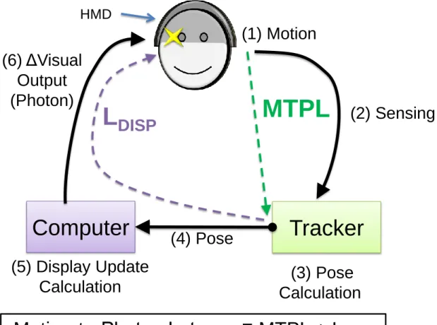
Figure 2: Motion-to-photon latency: schematic definition.
The user is wearing an AR head-mounted display (HMD) (center-top). When the user moves (1), this motion is sensed by the tracker’s sensors (2). The user’s new pose is calculated by the tracker (3) and a new pose appears on the tracker’s output (4). Schematically, motion-to-pose latency (MTPL) is the time interval from (1) to (4). A computer reads the new pose and calculates display updates (5). These updates are sent to the display whereupon the display’s visual output changes (6). Schematically, LDISP (display
2.1
Motion-to-Photon Latency: Definitions
The positions of virtual objects on an AR display are determined by the user’s head position and orientation – the user’s head pose. When virtual objects are meant to have definite positions with respect to the real world, these objects’ positions on the display must change as the user moves.
The user’s pose is measured by a tracker. A notional tracker is shown in Figure 1. The user (lower left) is shown wearing a head-mounted display (HMD). Sensors are located in the surrounding environment (top). The sensors are stimulated by emitters located on the HMD. We refer to the
combination of the HMD and the emitters as the tracked target. From time to time, a compute function (right) reads the sensors, performs calculations, and pose samples appear on the tracker’s output.
In simple terms, motion-to-photon latency is the time between a change in the user’s ground-truth pose (true pose) and a change in the AR display’s output corresponding to the user’s (new) pose. We can partition motion-to-photon latency into two distinct, disjoint components: the time taken for the tracker’s output to change in response to the change in true pose and the time taken for the display’s output to begin changing in response to the new tracker output.
Consider the figurative AR system in Figure 2. A user wearing an AR head-mounted display (HMD) is shown at the top of the figure, a tracker is shown at the lower right, and the computer
controlling the HMD is shown on the lower left. Six events, beginning with motion (1) and ending with a corresponding change in the display’s visual output (6), form a feedback loop beginning and ending with the user. The time to traverse this loop is the system’s motion-to-photon latency. We divide this time interval into two distinct, disjoint parts: motion-to-pose latency (MTPL) and “display latency” (LDISP ).
The timer for LDISP starts when the timer for MTPL ends, i.e., when a new pose sample appears on
the tracker’s output. Subsequently, this pose (4) is read by the computer. The computer calculates what should appear on the display based on the new pose (5). The computer then commands the display to change its visual output, e.g., a newly-rendered frame may be transmitted to a monitor. The timer for LDISP
stops when the display’s visual output begins changing in response to the new pose (6). LDISP can be
thought of as “pose-to-photon” latency or, more simply, as the sum of all non-tracking latency components (e.g., the time taken for the computer to read the new pose from of the tracker’s output, rendering time, the time taken to transmit the new image to the output device, and the output device’s response time). In this dissertation, the term “display latency” is interchangeable with LDISP, as defined
above, unless otherwise noted.
Motion-to-photon latency, then, is the sum of MTPL and LDISP.
Because of our precise definition of MTPL, and particularly our explicit inclusion of sensor-intrinsic latency, our definition of “motion-to-photon latency” may differ from this term’s exact meaning as used elsewhere in the literature. Other terms used in the literature, such as “end-to-end latency” and “system latency”, may or may not be equivalent to our definition of motion-to-photon latency. For example, Holloway defines the term “system delay” as, “…the sum of all the delays from the time the measurement of head position/orientation is made until the time that the image generated using that information is finally visible to the user… [emphasis added]” (R. L. Holloway 1997). It is not clear whether Holloway’s system delay includes sensor-intrinsic latency, such as the exposure time of a CMOS camera sensor or sensor-to-tracker data transfer time.
2.2
Latency in Augmented and Virtual Reality: Background
The effects of motion-to-photon latency and means of reducing latency in AR (and VR) systems have been the subject of considerable research. Olano, et al. (1995) vividly describe the effects of (high) motion-to-photon latency in VR HMDs as causing a “high viscosity world” – where the viewed world is constantly lagging behind one’s movements. Olano, et al. further note that the effect is even more pronounced in see-through AR because virtual objects lag behind the real world; the virtual objects appear to move with respect to the real world, making the effect that much more apparent to the user compared to VR. Studying users’ interactions with virtual objects in OST AR, Ellis, et al. (1997) found that rendering latency (which we categorize as a component of display latency), among other factors, was significantly detrimental to users’ experience and task performance (e.g., efficiency or accuracy in
performing a task). More recently, Nabiyouni, et al. (2017) found significant negative correlation between users’ performance in AR-based training tasks and motion-to-photon latency. Meehan, et al. (2003) show that latency has a negative effect upon presence; presence can be understood as a subjective assessment of how realistic and plausible the user finds the virtual experience.
Holloway (1995, 1997) performed a detailed analysis of the sources of registration errors in OST AR systems proposed for use in surgical planning; Holloway defines registration errors as misalignments between real and virtual objects. The total observed registration error can be understood as the net effect of a number of error sources; for our purposes, these error sources can be divided into two categories:
Static Errors: static errors are caused by factors including: static tracking errors, optical
distortion14, world-to-tracker calibration, and display non-linearity
Dynamic Errors: dynamic errors are primarily caused by what Holloway calls system delay,
the definition of which closely-resembles our definition of motion-to-photon latency. This is to say that latency is the proximate cause of dynamic registration errors (what we call disparities in dynamic position or real-virtual displacements).
According to Holloway’s analysis, system delay is by far the largest single contributor to registration errors. Holloway found that, in his OST AR system, system delay was responsible for real-virtual displacements15 of 20-60 mm at translational velocities of 500 mm/s or rotational velocities of 50°/s. Jerald (2009) performed user studies to measure the thresholds at which motion-to-photon latency becomes perceptible to users of a CRT projector-based system that simulated OST AR. Jerald found that some trained users were sensitive to latencies as small as 3 ms. Abrash (2013) suggests that designers of VR systems should target motion-to-photon latencies on the order of 1 ms. Zheng, et al. (2014) estimate a “perceptual floor” for motion-to-photon latency in VR systems in the range of 2-11 ms. Our assessment is that the consensus in the literature, writ large, is that, for motion-to-photon latency, “lower is better” in both AR and VR.
14 E.g., due to the lenses used in camera-based trackers. 15
Perceptual Thresholds
The just-noticeable difference thresholds for real-virtual displacement and motion-to-photon latency in OST AR are not well-characterized in the literature and the perceptual threshold for motion-to-photon latency is likely on the order of ten times lower in AR than in VR (see below).
2.3
Mitigating Display Latency Sources
The negative effects of motion-to-photon latency have led to substantial research into reducing or eliminating sources of latency. In general, each such work can be understood as addressing either MTPL or display latency. We discuss prior work relating to MTPL in section 4.2 and discuss display latency here. Recall that display latency (LDISP) is the time from a new pose sample appearing on the tracker’s
output to the corresponding change in the display’s visual output.
Consider an AR system where MTPL=0 and that any component of the system (such as a GPU or low-latency display controller) can obtain the user’s true pose at any time, instantly, with no data
transmission delay. In this imaginary system, display latency is the sole contributor to motion-to-photon latency. If the display is frame-based, i.e., each output image is calculated in its entirety and then transmitted to the output device on a frame boundary, the display’s latency will be, at minimum16, one frame period, i.e., the reciprocal of the frame rate.
We could imagine improving such a display’s performance by, perhaps, not waiting for the entire full frame to be ready, but instead transmitting it and/or beginning to scan it out as the computation proceeds. We have just (somewhat crudely) described one embodiment of frameless displays. Bishop, et al. (1994), with considerably more eloquence, identify the problem of frame-based displays (specifically the rendering component) and suggest frameless rendering as an alternative. Friston, et al. (2016) present a more modern approach to frameless rendering for a VR application. In principle, frameless rendering enables the display to continually update the pose it is using to calculate its output. This, to some extent,
16 We can imagine the “minimum” as where the image is transmitted to and appears on the display’s output
reduces motion-to-photon latency. This general technique is understood to be implemented in the Oculus™ Rift17, a VR HMD. We observe, however, that even if each pixel on the display’s output is perfect with respect to the user’s true pose, in a raster-scanned display, if the user is in motion, each pixel will fall ever-more out of alignment with the real world until it is updated. So the display latency of a raster-scanned display is still bounded by the frame rate.
Greer, et al. (2016) propose a method of driving organic light emitting diode (OLED) panels at effective frame rates in excess of 1 kHz. If one could framelessly-render to row-groups of such a panel in parallel, then the display latency could, in principle, be under 1 ms. Regan and Miller (2017) demonstrate a projective display based on a digital micromirror device (DMD) output device and outputting low-persistence binary (monochrome) frames at 2.88 kHz18; the issue of persistence, specifically, is
highlighted – that is, less real-virtual disparity is perceived if one reduces the time that a pixel remains in the “wrong” position (due to head movement).
Lincoln (2017) and Lincoln, Blate, et al. (2016) report on a DMD-based OST AR HMD with mean motion-to-photon latency of 80 μs. The underlying technique, described in detail in Lincoln (2017), is something of a hybrid of frame-based and frameless rendering: Video frames larger than the display’s resolution are rendered on a GPU and transmitted to the low-latency display controller (the system component driving the DMD) at 60 Hz. Mechanical tracking provides the display controller with poses about every 15 μs. What Lincoln calls a “post-rendering warp” – in this case a 2D translation – is
performed for every binary frame (at about 16 kHz), such that each frame is positioned based on the most current pose sample. Note that the underlying tracking sensor, an optical rotary encoder, has essentially zero latency. The 15 μs period (delay) is due to serial data transfer time; this is an implementation artifact
17
http://www.oculus.com
18 The integrated frame rate (see section 3.1) of Regan and Miller’s display is 120 Hz. Based on their description of
and is not intrinsic to Lincoln’s display proper19
. The display latency (LDISP) of Lincoln’s display minus
the time taken for the serial transfer of tracking data is on the order of 65 μs20.
2.4
Perceiving a Stationary World When One Moves
The optical combiner of an OST AR HMD is located in front of the user’s eye. Each of the display’s pixels occupies some fixed location referenced to the user’s head21
– independent of the user’s pose. For an object to be perceived as stationary relative to the real world, its location relative to the user’s head changes if and only if the user moves and the change in location is consistent with the user’s movement, as discussed below (Wallach 1987). For example, as one turns one’s head to the left, from the retina’s perspective, stationary objects appear to be translating towards the right22
. If the velocity of translation an object, from the retina’s perspective, is equal and opposite to the velocity of head rotation, the object is perceived as stationary; this is called immobility. If the velocity of translation is not equal and opposite to the velocity of head rotation – even by a small amount – the object is perceived as moving (non-stationary) [idem].
To maintain immobility for a semantically-stationary virtual object, the object’s position on the display must change whenever the user’s pose changes. Specifically, the virtual object must appear to translate with a velocity equal and opposite to that of the user’s head’s pose velocity. This is the perceptual mechanism by which real-virtual discrepancies in the dynamic locations of virtual objects – real-virtual translations during head rotation – break the perception of immobility.
19
Specifically, if the rotary encoder had been directly-coupled to the display controller hardware (FPGA), this 15 μs delay would disappear.
20 Many mechanical trackers, such as the rotary shaft encoders used in (Lincoln, Blate, et al. 2016) and (Lincoln,
Blate, et al. 2017), have essentially zero tracking latency; in these two examples, the mean tracking latency was about 15 μs because the encoders were read by an off-board decoder (an FPGA) and the values were transmitted to the display controller via a relatively low-speed (~2 Mbps) serial link. The latency intrinsic to the encoders themselves and decoding is on the order of 100 ns.
21 We assume that the HMD fits the user snugly, i.e., head-HMD orientation and alignment are invariant. A loose-or
poorly-fitting HMD may cause other real-virtual disparities; such disparities are beyond the scope of this dissertation.
22 The image on the retina is inverted, so, physically, “appear to be translating to the right” means that the image on
2.5
Perception of Latency in Optical See-Through Augmented Reality
In VR, motion-to-photon latency in excess of one video frame time is typically perceived as “swimming” – a perceptible lag between one’s movement and the display’s response. Importantly, in VR, everything in one’s FOV lags uniformly. In VR, research suggests that maintaining motion-to-photon latency on the order of single-digit milliseconds is sufficient to mitigate swimming or its higher-frequency relative, “judder” (Jerald 2009, Abrash 2013, Meehan, et al. 2003, Bishop, et al. 1994).
In OST AR, however, the virtual object is always visually-referenced to the surrounding real world. What appears as lag in VR – a delay between a head motion and the change in position of the virtual scene – appears in OST AR as a discontinuous movement of the virtual object with respect to the real world. Additionally, in the time between display updates, the virtual object appears to move in the direction of head movement – the exact opposite how a (real) stationary object would move relative to the retina. The conditions for immobility are violated and the user perceives that the virtual object is moving. For example, during head rotation (yaw, i.e., turning the head left and right) the virtual object appears to vibrate laterally. In our own experience, even with motion-to-photon latencies of about 1 ms and at relatively low rotational velocities (under 50°/s), this effect is clearly visible and profoundly unrealistic.
An increase in motion-to-photon latency and/or pose velocity23 will result in a larger real-virtual displacement. For head rotation in yaw and pitch, the magnitude of real-virtual angular displacements can be calculated directly: For example, if motion-to-photon latency is 16.7 ms (one frame period at 60 Hz), angular real-virtual displacement will be one arcminute per degree per second of head rotation.
We have demonstrated that sub-100 μs motion-to-photon latency eliminates perceptible real-virtual displacements during head rotations in excess of 300°/s in the ~16 kHz-binary-frame-rate display disclosed in (Lincoln, Blate, et al. 2016). Real-virtual discrepancies (i.e., between binary frames) still exist in the display reported in [idem]; apparently, these discrepancies are small enough, short enough, or both, so as to be imperceptible.
23
CHAPTER 3: MITIGATING DISPARITIES IN ILLUMINATION
To mitigate real-virtual discrepancies in the luminance of virtual objects, each object’s luminance should be made to be consistent with its real-world surroundings. For example, an object lying under a table in deep shade should appear darker than the same object brightly illuminated by a nearby table lamp. The range of luminance in a typical scene commonly spans five to six orders of magnitude
(100-120 dB24). Providing real-virtual consistency in object luminance, then, requires a display with commensurate luminous dynamic range25. Additionally, increased color enables enhanced real-virtual consistency in object color.
The present work introduces a new method for the illumination of binary frame spatial light modulator-based (BSLM) displays. An example of such a display is the low-latency optical see-through (OST) augmented reality (AR) display reported by Lincoln, Blate, et al. (2017). Central to our method is a high dynamic range, high-speed, variable intensity light source. In this method, the display controller26 can illuminate each binary frame with any color and intensity of light within the illuminator’s dynamic range. Our method, dynamic binary frame illumination (DBI), decouples spatial and intensity modulation, leading to exponentially more-efficient use of BSLMs’ high binary frame rates. DBI allows us to increase the display’s luminous dynamic range and color depth (bits-per-color) and reduce display latency.
24 Unless otherwise indicated, we use the field scale for dB (Decibels), i.e., 20 log
10 (fmax/fref), where fref is the
“reference” level, i.e., the minimum field strength, the noise floor, or a specific reference level (for example, dBmV is referenced to 1 mV).
25 Dynamic range is the ratio of a signal’s maximum strength to its minimum (non-zero) strength. For example, if a
lamp has a dimmer knob that allows its output to be varied between 1 and 250 lumens, then its dynamic range is 250:1 (about 48 dB referenced to one lumen).
26 The “display controller” can be understood as the set of electronics that controls the BSLM inclusive of the
In this chapter, we present the design, implementation, and evaluation of a DBI illuminator which uses high-speed, digitally-programmable current sources to drive high-intensity RGB (red, green, and blue) light emitting diodes (LEDs). This illuminator enables the display controller to illuminate any binary frame at any luminosity value within the illuminator’s 115 dB dynamic range.
We further present a prototype position-sensitive light sensor used to implement scene-adaptive lighting the low-latency OST AR display reported by Lincoln, Blate, et al. (2017). This sensor has over 140 dB of dynamic range and provides the display controller with real-time luminance measurements for four 9° slices of the scene (subtending the display’s approximately 34° field-of-view).
3.1
Introduction
Binary frame spatial light modulators, such as digital micromirror devices (DMDs) (Hornbeck 1991) and binary-frame liquid crystal on silicon (LCoS) devices (Forth Dimension 2018), produce 1-bit (monochrome) images – binary frames – at binary frame rates of 4-32 kHz. Human persistence of vision essentially performs time-domain integration of many binary frames, resulting in the perception of a continuous-tone image. The resulting continuous-tone image is an integrated frame. The integrated frame rate is equal to the binary frame rate divided by the number of binary frames per integrated frame.
Traditional BSLM displays typically27 use constant-intensity light sources; if the light source has intensity L, then each pixel of each binary frame has intensity zero or L. Suppose we want a pixel’s apparent intensity to be proportional to (v/2n)∙L, where v is an n-bit integer. In traditional displays, this is achieved by outputting 2n binary frames where the respective pixel is on for v frames. Digital synthesis of analog signals in this manner is known as pulse train modulation28 (PTM). Under PTM, the number of binary frames per integrated is equal to the number of possible intensity values, i.e., 2n: one binary frame per intensity value.
27
Some BSLM displays use bivalent light sources. See section 3.2.2.
28 Common embodiments of PTM include pulse width modulation (PWM), pulse density modulation (PDM), and
Our insight is that we can reduce the number of binary frames per integrated frame by varying the intensity at which each binary frame is illuminated. In particular, we require only n binary frames – one binary frame per bit of intensity depth. Beginning at the most-significant bit, the binary frames are illuminated at intensities { L, L/21, L/22, … L/2n-2, L/2n-1 }29, where L is the light source’s full-scale output intensity. A pixel is turned on in a given frame if its respective bit is one.
Our method, dynamic binary frame illumination (DBI), allows us to reduce and, in fact, optimize the number of binary frames per integrated frame: Specifically, using DBI, an n bit-per-pixel (bpp) integrated frame requires at most n binary frames30, each illuminated at a binary-weighted luminosity. DBI thus makes exponentially more-efficient use of the BSLM’s high frame rate. This has the immediate effect (versus PTM) of increasing the integrated frame rate by a factor of 2n/n. For example, to produce 8-bit grayscale integrated frames, PTM requires 28=256 binary whereas DBI requires 8 frames – an improvement of 256/8=64x. For 16-bit greyscale, PTM requires 216=65,536 binary frames whereas DBI requires only 16 frames – an improvement of 4096x.
Our illuminator uses a high-power LED with independent red, green, and blue (RGB) emitters integrated into a single package. Each emitter is driven by a high-speed, 16-bit-precision current source. Measured at the display’s exit optics (see Figure 7), our illuminator’s dynamic range is about 115 dB (~19 bits31). Our DBI implementation has been used in two AR displays. We originally designed and implemented a DBI illuminator to enable the low-latency, HDR, scene-adaptive display reported in (Lincoln, Blate, et al. 2017). In addition to the display of (Lincoln, Blate, et al. 2017), our DBI illuminator enabled the implementation of the novel volumetric near-eye display of (Rathinavel, et al. 2018). These two displays leverage aspects of DBI in different ways, providing examples of our method’s potential.
29
Note that for the same value of L, the absolute maximum intensity under PTM, L∙(2n-1)/2n ≈ L, is greater than the absolute maximum intensity under DBI, which is approximately 2∙L/n. This is discussed further in section 3.3.2.
30
DBI is optimal in the sense that, in the general case, n binary frames are required to reproduce the information contained in the n bpp input image.
31
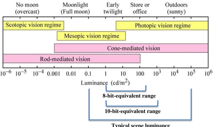
Figure 3: Dynamic range of human vision.
We consider typical scene luminance to be about 10-1 to 105 cd/m2 – approximately moonlight to daylight (cd is the abbreviation for the SI unit candela).
Figure adapted from (Stockman and Sharpe 2006).
~40mm
~120 μm
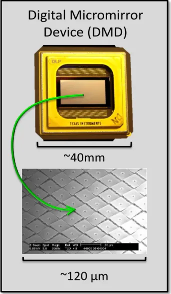
Digital Micromirror
Device (DMD)
Figure 4: Digital Micromirror Device (DMD): Example of device and micrograph of mirror array. Top: A DMD chip. Bottom: Micrograph of the surface of a DMD showing the microscopic, orientable mirrors.
Figure 5: Optical signal path of a color wheel-based DMD projector.
The projection lamp (i.e., light source) outputs white light which is filtered by the rotating color wheel. The wheel typically makes one revolution per output video frame. The “DLP® Chip” (DMD) is controlled by the display controller.
(Image © Texas Instruments)
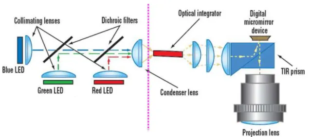
Figure 6: Optical signal path of LED-illuminated DMD projector.
3.2
Related Work and Background
3.2.1
High Dynamic Range Displays
HDR is generally understood to denote devices whose luminance and/or color depth exceeds that of standard 24-bit RGB (red, green, and blue). One industry definition of HDR is the UHD-10
specification (UHD Alliance Premium, Myszkowski, Mantiuk and Krawczyk 2008, Vandervell 2016), which specifies that a conformant display’s luminance must have a dynamic range of either 86 dB referenced to 5·10-2 cd/m2 for LED-based displays or 120 dB referenced to 5·10-4 cd/m2 for OLED-based displays32. The same specification requires that the display support 10 bits-per-color and must be able to display 90% of the P3 color space (gamut) (Masaoka and Nishida 2015).
Methods for increasing the dynamic range of displays have been pursued widely. Larson, Rushmeier and Piatko (1997) reported tone reproduction operator that uses aspects of human visual perception to create the appearance of an HDR scene with a standard dynamic range output device or medium. Myszkowski, Mantiuk and Krawczyk (2008) present a survey of HDR video, including image capture, representation, and reproduction (display). Whitehead, et al. (2007) disclose a method for producing HDR display devices using two spatial light modulators (SLMs) in series; the first SLM produces the full-resolution image at a reference luminosity and the second SLM, whose resolution is lower than that of the first SLM, adjusts the luminosity of regions of the image. In a similar manner, LCD displays with over 100 dB of dynamic range in luminance have been demonstrated. These LCD displays use an array of variable-intensity white backlights (as opposed to a monolithic backlight); the resolution of the backlight array is significantly less than that of the LCD itself, so each “pixel” in the backlight array sets the luminance for a region of the display (Torres 2005 and Brightside Technologies 2006). Methods for increasing color depth/gamut in DMD-based displays have also been proposed; Gibbon, et al. (2006) disclose a technique for increasing the dynamic range of DMD-based projection systems wherein two DMDs are used in series. The first DMD pre-modulates a constant-intensity light source,
32
producing variable intensities globally, regionally, or on a per-pixel basis; the second DMD spatially-modulates the (now variable-intensity) light in like manner to a traditional DMD-based display (see section 3.2.4).
3.2.2
Reducing Integrated Frame Times
Chang, Kumar, and Sankaranarayanan (2016) demonstrate up to 16-bit color depth DMD-based video projectors using an illumination method they call Hybrid Light Modulation (HLM). HLM combines PTM and variable-intensity illumination such that HDR video can be displayed without a reduction in integrated frame rate and with minimal impact to maximum intensity. HLM, as proposed and
implemented in [idem], cannot achieve the temporal performance of our method; among other factors, their variable-intensity, pulse-width modulated (PWM) light source has about 8 to 9 bits of precision; in comparison, our DBI implementation, described in section 3.3, has 16-bit precision.
Both HLM and DBI leverage variable-intensity light sources for the same basic purpose: to reduce the number of binary frames per integrated frame. DBI and HLM were independently-conceived for different purposes (OST AR versus video projectors, respectively) and optimize for different factors (low-latency versus maximum intensity, respectively).
low-order k bits), then the total number of binary frames per integrated frame drops to O(2n-k + 2k) – which is still exponential in n. In fairness, if we consider the best case, where k=n/2, only O(2∙2n/2
) binary frames are required per integrated frame; this is a significant savings.
3.2.3
The Human Element
The human visual system operates effectively over a large range of luminance – from
10-6 to 108 cd/m2—a total range of 280 dB (Stockman and Sharpe 2006, IDS Imaging 2009, and Lagunas, et al. 2017). Figure 3 depicts a subset of this range with contextual examples for several lighting levels. There does not appear to be general agreement on the dynamic range of “typical” scene lighting, but estimates of 100-120 dB are common [idem]. If we declare our reference luminance level to be moonlight (10-1 cd/m2), then, assuming a dynamic range of 120 dB, the maximum illumination level is sunlight (105 cd/m2). Due to the rate of adaptation of rod cells, particularly during desaturation, the full range of visual sensitivity is not available simultaneously (Pattanaik, et al. 2000). For example, if a scene’s
luminosity extends from 10-4 to 106 cd/m2, rod saturation will render the dimmer content invisible. Even if we could build a display with this dynamic range (200 dB), only a scene-dependent subset of this range would be perceptually-useful; that is, under any given lighting conditions, at most about 120 dB of the display’s dynamic range would be visible to the user and the remainder of the display’s dynamic range would be unused.
3.2.4
Binary Frame Displays and Digital Micromirror Device-Based Projectors
A binary frame is a one-bit monochrome image – each pixel is either fully-on or fully-off. In this dissertation, we assume that the binary frames are generated by reflective spatial light modulators