Available online throug
ISSN 2229 – 5046
NEW ITERATIVE NUMERICAL ALGORITHMS
FOR MINIMIZATION OF NONLINEAR FUNCTIONS
K. Karthikeyan*
School of Advanced Sciences, Mathematics Division VIT University, Vellore-632014, India.
(Received on: 03-11-12; Revised & Accepted on: 21-12-12)
ABSTRACT
I
n this paper, we propose few new algorithms, for minimization of nonlinear functions. Then comparative study among the new algorithms and Newton’s algorithm is established by means of various examples.Key words: Nonlinear functions; Newton’s method; Halley’s method; Modified Halley’s method; Order of convergence.
1. INTRODUCTION
In recent times, many problems in business situations and engineering designs have been modeled as an optimization problem for taking optimal decisions. Optimization problems with or without constraints arise in various fields such as science, engineering, economics, management sciences, etc., where numerical information is processed In fact, numerical optimization techniques have made deep in to almost all branches of engineering and mathematics.
Several methods [2, 12, 16] are available for solving unconstrained minimization problems. These methods can be classified in to two categories as non gradient and gradient methods. The non gradient methods require only the objective function values but not the derivatives of the function in finding minimum. The gradient methods require, in addition to the function values, the first and in some cases the second derivatives of the objective function. Since more information about the function being minimized is used through the use of derivatives, gradient methods are generally more efficient than non gradient methods. All the unconstrained minimization methods are iterative in nature and hence they start from an initial trial solution and proceed towards the minimum point in a sequential manner.
To solve unconstrained nonlinear minimization problems arising in the diversified field of engineering and technology, we have several methods to get solutions. For instance, multi-step nonlinear conjugate gradient methods [6], ABS-MPVT algorithm [15] are used for solving unconstrained optimization problems. A proximal bundle method with inexact data [17] is used for minimizing unconstrained non smooth convex function. A new algorithm [8] is used for solving unconstrained optimization problem with the form of sum of squares minimization.
Many iterative methods have been developed for solving nonlinear equations in recent years by using the Taylor series, decomposition techniques and quadrature formulae [1, 3-5, 7, 9, 13, 15, 18]. Noor and Noor [9] have suggested a sixth order predictor-corrector iterative type Halley method for solving nonlinear equations. Kou et.al. [10, 11] have also suggested a class of fifth order iterative methods. In these methods, one has to evaluate the second derivative of the function which is a draw back of these methods. Recently, Muhammad Aslam Noor et. al. [14] introduced fifth order modified predictor corrector Halley method by replacing the second derivatives of the function by its finite difference scheme to overcome the above mentioned drawback. In this paper, we introduce six new algorithms for minimization of non linear functions and comparative study is established among the new algorithms with Newton’s algorithm by means of examples.
2. NEW ALGORITHMS
In this section, we introduce six numerical algorithms for minimizing nonlinear real valued and thrice differentiable real functions.
Consider the nonlinear optimization problem: Minimize
{
f
(
x
),
x
∈
R
,
f
:
R
→
R
}
wheref
is a nonlinear thrice differentiable function.Consider the function
G
(
x
)
=
x
−(
g
(
x
)
g
′
(
x
)
)
whereg
(
x
)
=
f
′
(
x
)
. Here f(x) is the function to be minimized.)
(
x
G
′
is defined around the critical point x* of f(x) ifg
′
(
x
∗)
=
f
′′
(
x
∗)
≠
0
and is given by
Corresponding author: K. Karthikeyan*
)
(
)
(
)
(
)
(
x
g
x
g
x
g
x
G
′
=
′′
′
.If we assume that
g
′′
(
x
∗)
≠
0
, we haveG
′
(
x
∗)
= 0 iffg
(
x
∗)
=
0
.Consider the equation
g
(
x
)
=
0
(2.1)whose one or more roots are to be found.
y
=
g
(
x
)
represents the graph of the functiong
(
x
)
and assume that an initial estimatex
0 is known for the desired root of the equationg
(
x
)
=
0
.Here we consider iterative techniques to find the simple root of a non linear equation g(x) = 0 where
g
:
D
⊂
R
→
R
for an open interval D is a scalar function.Let α be a simple real zero of a real function and let x0 be an initial approximation to α. By using Taylor’s series, we
have
0
...
!
2
)
(
)
(
)
(
)
(
)
(
00 0
0
0
+
=
−
′′
+
−
′
+
g
x
x
x
g
x
x
x
x
g
(2.2)From the above equation (2.2) we have the following new methods.
New method – I
For a given x0, we get xn+1 by the following iterative schemes
)
(
)
(
)
(
2
)
(
)
(
2
2 1
n n
n
n n n
n
x
g
x
g
x
g
x
g
x
g
x
x
′′
−
′
′
−
=
+ (2.3)
Since
g
(
x
)
=
f
′
(
x
)
the equation (2.3) becomesNew Algorithm – I
)
(
)
(
)
(
2
)
(
)
(
2
2 1
n n
n
n n
n n
x
f
x
f
x
f
x
f
x
f
x
x
′′′
′
−
′′
′′
′
−
=
+ (2.4)
The order of convergence of the new algorithm – I is three which is based on Halley’s method [7, 13].
New method – II
We introduce New method – II which is based on Noor and Noor [9] two step method.
For a given x0, we get xn+1 by the following iterative schemes
)
(
)
(
n n n
n
x
g
x
g
x
y
′
−
=
)
(
)
(
)
(
2
)
(
)
(
2
2 1
n n
n
n n n
n
y
g
y
g
y
g
y
g
y
g
y
x
′′
−
′
′
−
=
+ (2.5)
Since
g
(
x
)
=
f
′
(
x
)
the equation (2.5) becomesNew Algorithm –II
)
(
)
(
n n n
n
x
f
x
f
x
y
′′
′
−
=
)
(
)
(
)
(
2
)
(
)
(
2
2 1
n n
n
n n
n n
y
f
y
f
y
f
y
f
y
f
y
x
′′′
′
−
′′
′′
′
−
=
+ (2.6)
In the equation (2.5), to make it free from second derivative of the function g we consider
n n n
x
y
x
g
y
g
y
g
−
′
−
′
=
Combining (2.5) and (2.7) we have the following new method which is two step modified Halley’s method for the function g. The order of convergence is fifth order which is clear from the following theorem 3.1.
New method – III
For a given x0, we get xn+1 by the following iterative schemes
)
(
)
(
n n n nx
g
x
g
x
y
′
−
=
)
(
)
(
)
(
)
(
)
(
)
(
)
(
2
)
(
)
(
)
(
2
2 2 1 n n n n n n n n n n n ny
g
y
g
x
g
y
g
x
g
y
g
x
g
y
g
y
g
x
g
y
x
′
′
+
′
−
′
′
−
=
+ (2.8)
Since
g
(
x
)
=
f
′
(
x
)
the equation (2.8) becomesNew Algorithm –III
)
(
)
(
n n n nx
f
x
f
x
y
′′
′
−
=
)
(
)
(
)
(
)
(
)
(
)
(
)
(
2
)
(
)
(
)
(
2
2 2 1 n n n n n n n n n n n ny
f
y
f
x
f
y
f
x
f
y
f
x
f
y
f
y
f
x
f
y
x
′
′′
′′
+
′
′′
−
′′
′
′′
′
′
−
=
+ (2.9)
We introduce the following new method-IV which is based on Noor et. al. [3] a two step Halley method of fifth order of convergent.
New method – IV
For a given x0, we get xn+1 by the following iterative schemes
)
(
)
(
)
(
2
)
(
)
(
2
2 n n n n n n nx
g
x
g
x
g
x
g
x
g
x
y
′′
−
′
′
−
=
)
(
)
)
(
)
(
(
)
(
2
)
(
))
(
)
(
(
2
2 1 n n n n n n n n nx
g
y
g
x
g
x
g
x
g
y
g
x
g
x
x
′′
+
−
′
′
+
−
=
+ (2.10)
Since
g
(
x
)
=
f
′
(
x
)
the equation (2.10) becomesNew Algorithm –IV
)
(
)
(
)
(
2
)
(
)
(
2
2 n n n n n n nx
f
x
f
x
f
x
f
x
f
x
y
′′′
′
−
′′
′′
′
−
=
)
(
)
)
(
)
(
(
)
(
2
)
(
))
(
)
(
(
2
2 1 n n n n n n n n nx
f
y
f
x
f
x
f
x
f
y
f
x
f
x
x
′′′
′
+
′
−
′′
′′
′
+
′
−
=
+ (2.11)
We introduce the following new method-V and VI which are based on the fifth order convergence methods of Kou et. al. [10, 11]
New method – V
For a given x0, we get xn+1 by the following iterative schemes
)
(
)
(
)
(
2
)
(
2
)
(
)
(
)
(
)
(
3 2 n n n n n n n n n nx
g
x
g
x
g
x
g
x
g
x
g
x
g
x
g
x
y
′′
′
−
′
′′
−
′
−
=
)
(
)
(
)
(
)
(
1 n n n n n n nx
y
x
g
x
g
y
g
y
x
−
′′
+
′
−
=
+ (2.12)
New Algorithm –V
)
(
)
(
)
(
2
)
(
2
)
(
)
(
)
(
)
(
3
2
n n
n n
n n
n n n
n
x
f
x
f
x
f
x
f
x
f
x
f
x
f
x
f
x
y
′′′
′′
′
−
′′
′′′
′
−
′′
′
−
=
)
(
)
(
)
(
)
(
1
n n n n
n n
n
x
y
x
f
x
f
y
f
y
x
−
′′′
+
′′
′
−
=
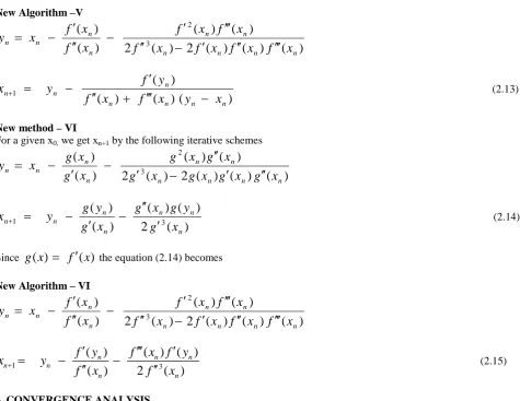
+ (2.13)
New method – VI
For a given x0, we get xn+1 by the following iterative schemes
)
(
)
(
)
(
2
)
(
2
)
(
)
(
)
(
)
(
3
2
n n n n
n n
n n n
n
x
g
x
g
x
g
x
g
x
g
x
g
x
g
x
g
x
y
′′
′
−
′
′′
−
′
−
=
)
(
2
)
(
)
(
)
(
)
(
3 1
n n n
n n n
n
x
g
y
g
x
g
x
g
y
g
y
x
′
′′
−
′
−
=
+ (2.14)
Since
g
(
x
)
=
f
′
(
x
)
the equation (2.14) becomesNew Algorithm – VI
)
(
)
(
)
(
2
)
(
2
)
(
)
(
)
(
)
(
3
2
n n
n n
n n
n n n
n
x
f
x
f
x
f
x
f
x
f
x
f
x
f
x
f
x
y
′′′
′′
′
−
′′
′′′
′
−
′′
′
−
=
1 3
(
)
(
)
(
)
(
)
2
(
)
n n n
n n
n n
f
y
f
x
f
y
x
y
f
x
f
x
+
′
′′′
′
=
−
−
′′
′′
(2.15)3. CONVERGENCE ANALYSIS
Here we consider the convergence criteria of the New method III and hence we have the convergence analysis of algorithm-III.
Theorem 3.1: Let
α
∈
I
be a simple zero of sufficiently differentiable functiong
:
I
⊆
R
→
R
for an open interval I. If x0 is sufficiently close to α, then algorithm 2.8 has fifth order of convergence.Proof: The proof of this theorem follows as in convergence theorem [14] and hence the order of convergence of the algorithm 2.9.
4. NUMERICAL ILLUSTRATIONS
Example 4.1: Consider the function
f
(
x
)
=
x
3−
2
x
−
5
. The minimized value of the function is 0.816497. The following table depicts the number of iterations needed to converge to the minimized value for all the new algorithms with three initial values x0 = 1, x0 = 2 and x0 = 3.Table – I: shows a comparison between the New iterative Algorithms and Newton’s Algorithms
Sl. No Methods For initial value x0 =1.000000
For initial value x0 =2.000000
For initial value x0 =3.000000
1 Newton’s Algorithm 3 5 5
2 New Algorithm-I 2 3 3
3 New Algorithm-II 2 2 2
4 New Algorithm-III 2 2 2
5 New Algorithm-IV 2 2 3
6 New Algorithm-V 2 2 2
7 New Algorithm-VI 2 2 3
Table – II: shows a comparison between the New iterative Algorithms and Newton’s Algorithms
Sl. No Methods For initial value x0 =1.000000
For initial value x0 =2.000000
For initial value x0 =3.000000
1 Newton’s Algorithm 7 8 10
2 New Algorithm-I 4 4 5
3 New Algorithm-II 3 3 4
4 New Algorithm-III 3 3 3
5 New Algorithm-IV 3 4 4
6 New Algorithm-V - - -
7 New Algorithm-VI - - -
Example 4.3: Consider the function
f
(
x
)
=
x
5+
x
4+
4
x
2−
15
. The minimized value of the function is 0.0000. The following table depicts the number of iterations needed to converge to the minimized value for all the new algorithms with three initial values x0 = 1, x0 = 2 and x0 = 3.Table – III: shows a comparison between the New iterative Algorithms and Newton’s Algorithms
Sl. No Methods For initial value x0 =1.000000
For initial value x0 =2.000000
For initial value x0 =3.000000
1 Newton’s Algorithm 5 6 8
2 New Algorithm-I 3 5 5
3 New Algorithm-II 2 3 3
4 New Algorithm-III - - -
5 New Algorithm-IV 3 4 5
6 New Algorithm-V - 3 -
7 New Algorithm-VI 4 5 6
Example 4.4: Consider the function
f
(
x
)
=
x
4−
x
−
10
. The minimized value of the function is 0.629961. The following table depicts the number of iterations needed to converge to the minimized value for all the new algorithms with three initial values x0 = 1, x0 = 2 and x0 = 3.Table – IV: shows a comparison between the New iterative Algorithms and Newton’s Algorithms
Sl. No Methods For initial value x0 =1.000000
For initial value x0 =2.000000
For initial value x0 =3.000000
1 Newton’s Algorithm 4 6 7
2 New Algorithm-I 3 4 5
3 New Algorithm-II 2 3 3
4 New Algorithm-III 2 3 3
5 New Algorithm-IV 2 3 3
6 New Algorithm-V 2 3 3
7 New Algorithm-VI 2 3 3
Example 4.5: Consider the function
f
(
x
)
=
e
x−
3
x
2. The minimized value of the function is 0.20448. The following table depicts the number of iterations needed to converge to the minimized value for all the new algorithms with three initial values x0 = −1, x0 = 0, and x0 = 1.Table – V: shows a comparison between the New iterative Algorithms and Newton’s Algorithms
Sl. No Methods For initial value x0 =−1.000000
For initial value x0 =0.000000
For initial value x0 =1.000000
1 Newton’s Algorithm 3 3 4
2 New Algorithm-I 3 2 3
3 New Algorithm-II 2 1 2
4 New Algorithm-III 2 1 2
5 New Algorithm-IV 2 2 2
6 New Algorithm-V 2 2 2
5. CONCLUSION
In this paper, we have introduced six numerical algorithms namely, New Algorithm –I, New Algorithm – II, New Algorithm – III, New Algorithm – IV, New Algorithm – V, New Algorithm – VI for minimization of non linear functions. From the above illustrations it is clear that the rate of convergence of these new algorithms is faster than Newton’s Algorithm. In real life problems, the variables can not be chosen arbitrarily rather they have to satisfy certain specified conditions called constraints. Such problems are known as constrained optimization problems. In near future, we have a plan to extend the proposed new algorithms to constrained optimization problems.
REFERENCES
[1]. S. Amat, S. Busquier and J.M. Gutierrez, Geometric construction of iterative functions to solve nonlinear equations, J. Comput. Appl. Math., 157(2003), 197–205.
[2]. Andrei, N, A scaled nonlinear conjugate gradient algorithm for unconstrained Optimization, Optimization, 57(4)(2008), 549 – 570.
[3]. M. Aslam Noor and K. Inayat Noor, Fifth-order iterative methods for solving nonlinear equations’, Appl. Math. Comput. (2006) doi:10.1016/j.amc.2006.10.007.
[4]. J.A. Ezquerro and M.A. Hernandez, A uniparametric Halley-type iteration with free second derivative’, Int. J. pure Appl. Math., 6 (1) (2003), 103–114.
[5]. J.A. Ezquerro and M.A. Hernandez, On Halley-type iterations with free second derivative, J. Comput. Appl. Math., 170(2004), 455–459.
[6]. J.A.Ford, Y. Narushima and H.Yabe, Multi-step nonlinear conjugate gradient methods for constrained minimization’, Computational Optimization and application, 40(2), 191 -216.
[7]. E.Halley, A new exact and easy method for finding the roots of equations generally and without any previous reduction’, Phil. Roy. Soc. London 18(1964) 136–147.
[8].Y.Hu, H. Su, and J. Chu, Conference proceedings IEEE international conference on systems, man and cybernetics, 7(2004), 6108 – 6112,
[9]. K. Inayat Noor, M. Aslam Noor, Predictor–corrector Halley method for nonlinear Equations, Appl. Math. Comput.,
in press, doi:10.1016/j.amc.11.023.
[10]. Jisheng Kou and Yitian Li, Improvements of Chebyshev–Halley methods with fifth order convergence, Appl. Math. Comput. (2006) doi:10.1016/j.amc.2006.09.097.
[11]. Jisheng Kou, Yitian Li and Xiuhua Wang, A family of fifth-order iterations composed of Newton and third-order methods, Appl. Math. Comput.(2006)doi:10. 1016/ j.amc. 2006.07.150.
[12]. Mohan C Joshi and Kannan M Moudgalya, 2004, Optimization theory and Practice, Narosa Publication House, New Delhi.
[13]. A. Melman, Geometry and convergence of Halley’s method’, SIAM Rev., 39 (4), (1997), 728–735.
[14]. Muhammad Aslam Noor, Waseem Asghar Khan and Akhtar Hussain, A new modified Halley method without second derivatives for nonlinear equation’, Appl. Math. Comput 189, (2007), 1268-1273.
[15].Pang, L.P., Spedicato, E., Xia, Z.Q. and Wang, W, A method for solving the system of linear equations and linear inequalities’, Mathematical and Computer Modelling, .46(5-6), (2007), 823 – 836.
[16]. G.V. Reklaitis, A. Ravindran and K.M. Ragsdell, 1983, ‘Engineering optimization methods and applications ’, John Wiley and sons, New York,
[17]. J. Shen, Z.Q Xia and L.P. Pang, A proximal bundle method with inexact data for convex non differentiable minimization, Nonlinear Analysis, Theory, Methods and Applications, 66(9)(2007), 2016 -2027.
[18]. J.F. Traub, 1964, Iterative Methods for Solution of Equations, Prentice-Hall, Englewood, Cliffs, NJ.