Vol 10, No 3 (2019)

Available online throug

On p-k Gamma Distribution

M. R. MAHMOUD AND R. M. MANDOUH*

Institute of Statistical Studies and Research, Cairo University, Egypt.

(Received On: 07-01-19; Revised & Accepted On: 11-03-19)

ABSTRACT

U

Keywords: The p-k Gamma function; the k Gamma function; the p-k Gamma distribution; the k Gamma distribution; maximum likelihood estimates; asymptotic variance-covariance matrix.

1. INTRODUCTION

In applied statistical work, popular distributions are modified and/or generalized using different directions. These directions are interested in deriving new distributions of univariate continuous distributions by introducing one or more additional shape parameter(s) to the baseline distribution. The Gamma (the Pearson type III) distribution is certainly among the most popular distributions. So we introduce a new general form of the gamma distribution through p-k gamma function defined by Gehlot (2017). Gehlot(2017) defined p-k gamma function as follows:

Г

𝑝 𝑘(𝑚) =� 𝑥𝑚−1𝑒−𝑥

𝑘

𝑝 �

∞

0 𝑑𝑥, 𝑝,𝑘> 0,𝑎𝑛𝑑𝑅𝑒(𝑚) > 0.

(1)

This function contains the k-gamma function(with parameters m and k) as a particular case for p=k (Diaz and Pariguan, 2007) and the gamma function(with parameter m) when p=k=1. In the next section we review some definitions and notation used to obtain our results.

2. BASIC DEFINITIONS AND NOTATION

The Pochhammer symbol: The Pochhammer symbol or the rising factorial function (𝑚)_𝑛 takes the form

(𝑚)𝑛=𝑚(𝑚+ 1)(𝑚+ 2) … (𝑚+𝑛 −1);𝑓𝑜𝑟𝑛 ≥1, (𝑚)0= 1,𝑚 ≠0. (2)

The Gamma Function: Let 𝑚 ∈ ℂ; the Euler gamma function Г(𝑚) is defined by

Г(𝑚) = lim_𝑛→∞𝑛₍!_𝑚𝑛𝑚−1₎

𝑛 .

(3)

and the integral representation of gamma function is

Г(𝑚) =� 𝑥∞ 𝑚−1_𝑒−𝑥_{𝑑𝑥, 𝑅𝑒(𝑚) > 0}

0 .

(4)

An important and useful property of the gamma function is given by

Г(𝑚+ 1) =𝑚Г(𝑚), (5)

and it is related to the Pochhammer symbol through

The Beta Function: The beta function 𝐵(𝑚₁,𝑚₂) is given by

𝐵(𝑚1,𝑚2) =� 𝑥𝑚1−1(1− 𝑥)𝑚2−1 1

0 𝑑𝑥, 𝑅𝑒(𝑚1) > 0,𝑅𝑒(𝑚2) > 0.

(7)

The beta function can be expressed in terms of gamma function as follows

𝐵(𝑚1,𝑚2) =Г_Г(₍𝑚_𝑚1)Г(𝑚2) 1+𝑚2).

(8)

For more details about these special functions and others such as hypergeometric function see Rainville (1960).

The Zeta Function: The Riemann’s zeta function is defined by the series

𝜁(𝑠) =�_𝑛1_𝑠, 𝑅𝑒(𝑠) > 1. ∞

𝑛=1

(9)

For more details about Riemann’s zeta function and other special functions see Temme (1996).

The Hurwitz zeta function is given by

𝜁(𝑚,𝑠) =� 1

(𝑛+𝑚)𝑠, 𝑚> 0.

∞

𝑛=0

(10)

when m=1 it gives the Riemann’s zeta function defined in (9) (see Andrews et al. (1999).

D𝚤́az and Pariguan (2007) introduced k-Pochhammer symbol (𝑚)_𝑛,𝑘, k-Gamma function Г_𝑘(𝑚), k-Beta function

𝐵𝑘(𝑚). They proved several identities for (𝑚)𝑛,𝑘, Г𝑘(𝑚) and 𝐵𝑘(𝑚). These identities were considered as a general

form of identities satisfied by the classical Pochhammer symbol, gamma function and beta function. They also provided the integral representation for the Г_𝑘(𝑚) and 𝐵_𝑘(𝑚).

The k-Pochhammer symbol: Let 𝑚 ∈ ℂ, 𝑘 ∈ ℝ and 𝑛 ∈ ℕ+, the k-Pochhammer symbol is given by (𝑚)𝑛,𝑘=𝑚(𝑚+𝑘)(𝑚+ 2𝑘) … … … (𝑚+ (𝑛 −1)𝑘).

The k-Gamma Function: For k > 0, the k-gamma function Г_𝑘 is

Г𝑘(𝑚) = lim_𝑛→∞𝑛!𝑘

𝑛_(𝑛𝑘)𝑚_{𝑘 −1}

(𝑚)𝑛,𝑘 , 𝑚 ∈ ℂ|𝑘ℤ

−_{. (11)}

with an integral form of k-Gamma function given by

Г_𝑘(𝑚) =� 𝑥∞ 𝑚−1_𝑒−𝑥𝑘/𝑘_{𝑑𝑥, 𝑓𝑜𝑟𝑚 ∈ ℂ, 𝑅𝑒(𝑚) > 0}

0 .

(12)

Some Properties of k-gamma function:

Г_𝑘(𝑚+𝑘) =𝑚Г_𝑘(𝑚).

(𝑚)𝑛,𝑘 =Г𝑘(_Г𝑚+𝑛𝑘) 𝑘(𝑚) .

Г_𝑘(𝑘) = 1.

Г_𝑘(𝑚) =𝑎𝑚𝑘∫ 𝑥∞ 𝑚−1𝑒−𝑥𝑘𝑘𝑎𝑑𝑥

0 ,𝑓𝑜𝑟𝑎 ∈ ℝ.

For more properties of k-gamma function see D𝚤́az and Pariguan (2007).

The k-Beta Function: The k-beta function 𝐵_𝑘(𝑚₁,𝑚₂) is given by

𝐵𝑘(𝑚1,𝑚2) =Г_Г𝑘(𝑚1)Г𝑘(𝑚2)

𝑘(𝑚1+𝑚2) , 𝑅𝑒(𝑚1) > 0, 𝑅𝑒(𝑚2) > 0.

The k-beta function satisfies the following identities:

𝐵𝑘(𝑚1,𝑚2) =� 𝑥𝑚1−1(1 +𝑥𝑘)−𝑚

1+𝑚2

𝑘

∞

0 𝑑𝑥.

𝐵𝑘(𝑚1,𝑚2) =_𝑘1� 𝑥𝑚1/𝑘−1(1− 𝑥𝑘) 𝑚2

𝑘 −1 1

0 𝑑𝑥.

𝐵𝑘(𝑚1,𝑚2) =1_𝑘𝐵(𝑚1/𝑘,𝑚2/𝑘). (14)

𝐵𝑘(𝑚1,𝑚2) =(𝑚_𝑚1+𝑚2) 1𝑚2 �

𝑛𝑘(𝑛𝑘+𝑚1+𝑚2)

(𝑛𝑘+𝑚1)(𝑛𝑘+𝑚2) .

∞

𝑛=0

The k-Zeta Function: The k-zeta function is defined by

𝜁𝑘(𝑚,𝑠) =�_(𝑚+1_𝑖𝑘)𝑠, 𝑓𝑜𝑟𝑘,𝑚> 0 𝑎𝑛𝑑𝑠> 0.

∞

𝑛=0

(15)

The k-zeta function satisfies the following identities:

𝜁𝑘(𝑚, 2) =𝜕𝑚2(𝑙𝑜𝑔Г(𝑚)).

𝜕𝑚2(𝜕𝑠𝜁𝑘)|𝑠=0=−𝜕𝑚2(𝑙𝑜𝑔Г(𝑚)). 𝜕𝑚𝑟(𝜕𝑠𝜁𝑘(𝑚,𝑠)) =−𝑚(𝑠)𝑟� 𝑖

𝑟

(𝑚+𝑖𝑘)𝑟+𝑠.

∞

𝑖=0

Also, D𝚤́az and Pariguan (2007) discussed Hypergeometric function in view of the k-Pochhammer symbol. For more details see their article.

Gelton (2017) introduced the two parameter Pochhammer symbol, two parameter gamma function and two parameter beta function and named them, as p-k Pochhammer symbol, _𝑝(𝑚)_𝑛,𝑘, p-k gamma function, _𝑝Г_𝑘 and p-k beta

function, _𝑝𝐵_𝑘(𝑚,𝑛) respectively.

The p-k Pochhammer symbol: Let 𝑚 ∈ ℂ;𝑘,𝑝 ∈ ℝ+𝑎𝑛𝑑𝑅𝑒(𝑚) > 0,𝑛 ∈ ℕ, the The p-k Pochhammer symbol (i.e. Two Parameter Pochhammer Symobol), _𝑝(𝑚)_𝑛,𝑘 takes the form

(𝑚)𝑛,𝑘,

𝑝 = (𝑚𝑝_𝑘 )(𝑚𝑝_𝑘 +𝑝)(𝑚𝑝_𝑘 + 2𝑝) … … … (𝑚𝑝_𝑘 + (𝑛 −1)𝑝).

and the relation between p-k Pochhammer symbol, k-Pochhammer symbol and classical Pochhammer symbol is (𝑚)𝑛,𝑘,

𝑝 =�𝑝_𝑘� 𝑛

(𝑚)𝑛,𝑘 = (𝑝)𝑛(𝑚_𝑘)𝑛.

The p-k Gamma Function: Let 𝑚 ∈ ℂ/𝑘ℤ−; 𝑘,𝑝 ∈ ℝ+−0 and Re(m) > 0, n ∈ ℕ, the p-k Gamma Function (i.e. Two Parameter Gamma Function), _𝑝Г_𝑘(𝑚) is given by

Г𝑘 𝑝 (𝑚) =

1

𝑘𝑛→lim∞

𝑛!𝑝𝑛+1_(𝑛𝑝)𝑚_{𝑘 −1}

(𝑚)𝑛,𝑘 𝑝 (𝑚) ,

(16)

with the following integral representation of p-k Gamma function

Г_𝑘

𝑝 (𝑚) =� 𝑥𝑚−1𝑒−𝑥

𝑘_/𝑝

∞

0 𝑑𝑥.

(17)

The relation between p-k gamma function, k- gamma function and classical gamma function is given by

Г_𝑘

𝑝 (𝑚) =� 𝑝 𝑘�

𝑚 𝑘_Г

𝑘(𝑚) =𝑝 𝑚

𝑘 𝑘 Г�

𝑚 𝑘�.

(18)

and the relation between p-k Pochhammer symbol and p-k gamma function take the form

(𝑚)𝑛,𝑘 =

Г_𝑘

𝑝 (𝑚+𝑛𝑘)

Г_𝑘

𝑝 (𝑚)

and the _𝑝𝐵_𝑘(𝑚₁,𝑚₂) function satisfies the following identities

𝐵𝑘

𝑝 (𝑚1,𝑚2) =1_𝑘� 𝑥 𝑚1

𝑘 −1(1− 𝑥)𝑚𝑘 −12 1

0 𝑑𝑥.

𝐵𝑘

𝑝 (𝑚1,𝑚2) =1_𝑘� 𝑥 𝑚1

𝑘 −1(1− 𝑥)𝑚𝑘 −12

(𝑥+ 1)𝑚1+𝑚𝑘 2 1

0 𝑑𝑥.

𝐵𝑘

𝑝 (𝑚1,𝑚2) =1_𝑘� 𝑥 𝑚1

𝑘 −1(1 +𝑥𝑘)−𝑚1+𝑚𝑘 2

∞

0 𝑑𝑥.

𝐵𝑘

𝑝 (𝑚1,𝑚2) =1_{𝑘 𝐵}(𝑚_𝑘1,𝑚_𝑘2). ₍₂₀₎

The p-k Psi Function: The logarithmic derivative of the p-k Gamma function is known as p-k Psi function, _𝑝𝜓_𝑘(𝑚)

𝜓𝑘

𝑝 (𝑚) =_𝑑𝑚𝑑 ln�𝑝Г𝑘(𝑚)�=

1

Г_𝑘

𝑝 (𝑚) 𝑑

𝑑𝑚�𝑝Г𝑘(𝑚)�. (21)

and

ln�_𝑝Г_𝑘(𝑚)�=� 𝜓𝑝 𝑘(𝑚) 𝑚

1 𝑑𝑥.

(22)

Some properties of _𝑝𝜓_𝑘(𝑚) are given by

𝜓𝑘

𝑝 (𝑚) =𝑙𝑛𝑝_𝑘 +𝜓 �𝑚_𝑘�. (23)

𝜓𝑘

𝑝 (𝑚) =𝑙𝑛𝑝_{𝑘 − 𝛾 −𝑚}𝑘 +𝑚 � _𝑖(𝑚1_+𝑖𝑘)

∞

𝑖=1 .

(24)

𝜓𝑘

𝑝 (𝑚) =𝑙𝑛𝑝_{𝑘 − 𝛾}+ (𝑚 − 𝑘)� _{(𝑖+ 1)(}1_{𝑚+𝑖𝑘)}

∞

𝑖=0 .

(25)

where 𝛾 is Euler’s constant and ψ(m) is classical Psi function. The r th derivative of p-k Psi function, _𝑝𝜓_𝑘(𝑚) obtained in terms of k-Zeta function, 𝜁_𝑘(𝑚,𝑟) as follows

𝑑𝑟

𝑑𝑚𝑟�ln [𝑝𝛾𝑘(𝑚)]�= 𝑑

𝑟−1

𝑑𝑚𝑟−1 𝑝𝜓𝑘(𝑚) = (−1)𝑟𝑘(𝑟 −1)!𝜁𝑘(𝑚,𝑟), for r≥2 (26)

where k-Zeta function is defined by

𝜁𝑘(𝑚,𝑟) =∑∞𝑖=0_{(𝑚+𝑖𝑘}1 ₎𝑟. (27)

For more details about p-k Pochhammer symbol, p-k Gamma function, p-k Beta function, p-k Psi function and p-k Hypergeometric function see Gehlot (2017).

Using p-k gamma function studied by Gehton(2017), we introduce p-k gamma distribution with four parameters in the following section.

3. p-k Gamma Distribution

We say that the random variable X follows a p-k gamma distribution with four parameters m, λ, k and p if it has a density function of the form

𝑓(𝑥) = _Г𝜆−𝑚

𝑘 𝑝 (𝑚)𝑥

𝑚−1_𝑒−(𝑥/𝜆)𝑘_/𝑝

, 𝑚,𝑝,𝑘 𝑎𝑛𝑑𝜆> 0, (28)

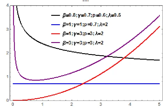
From (2 ) if λ = 1, we g et p-k-gamma distribution with three parameters. If p=k and λ = 1, we have k-gamma distribution with two parameters (Rahman et al. (2017). If p=k=1, we have gamma distribution with two parameter. So the results obtained in this paper are general form for three distributions. Plots of the pdf of the p-k gamma distribution for different parameter values are given in figure (1).

The density (2) of the p-k gamma distribution is decreasing, for 0 < m < 1 and unimodal, for m > 1, with mode at the point

𝑥= ((𝑚 −_𝑘1)𝑝𝜆𝑘)1/𝑘 (29)

Figure-1: Probability density function of p-k Gamma distribution for different values of the parameters

The CDF of p-k gamma distribution takes the form

𝐹(𝑥) = _Г𝜆−𝑚

𝑘 𝑝 (𝑚)∫ 𝑥

𝑚−1_𝑒−(𝑥/𝜆)𝑘/𝑝 𝑥

0 𝑑𝑥

=_Г(𝑚1_/𝑘)𝛾(𝑚/𝑘, (𝑥/𝑘)𝑘_/𝑝). (30)

where 𝛾(𝑚/𝑘, (𝑥/𝑘)𝑘/𝑝) is incomplete gamma function. One can note that cdf does not have closed form but one can put it in expansion form as follow:

𝐹(𝑥) = _Г1

𝑘 𝑝 (𝑚)∑

(−1)𝑖𝑝𝑖𝑥𝑚+𝑖𝑘

𝑖!𝜆𝑚+𝑖𝑘_{(𝑚+𝑖𝑘)}

∞

𝑖=0 . (31)

The Hazard Rate Function of p-k gamma distribution: The hazard rate function of p-k gamma distribution is given by

ℎ(𝑥) =

𝜆−𝑚

Г_𝑘

𝑝 (𝑚)

𝑥𝑚−1_𝑒−(𝑥/𝜆)𝑘/𝑝

1− 𝜆−𝑚

Г_𝑘

𝑝 (𝑚)

∫ 𝑥𝑥 𝑚−1_𝑒−(𝑥/𝜆)𝑘/𝑝 0 𝑑𝑥

, 𝑚,𝑝,𝑘 𝑎𝑛𝑑 𝜆> 0. (32)

Figure (2) illustrates possible shapes of (32) for selected parameter values. The shape appears increasing for (m > 1), constant for (p, k = 1), decreasing for (m < 1 and k < 1) and bathtub for (m < 1 and k < 1.)

The r th moment of p-k gamma distribution is given by:

𝐸(𝑋𝑟₎

= 𝜆−𝑚

Г_𝑘

𝑝 (𝑚)

� 𝑥∞ 𝑚+𝑟−1_𝑒−(𝑥/𝜆)𝑘/𝑝

0 𝑑𝑥

= 𝜆𝑟

Г_𝑘

𝑝 (𝑚)

� 𝑦∞ 𝑚+𝑟−1_𝑒−𝑦𝑘/𝑝

0 𝑑𝑥

=𝜆

𝑟 _Г

𝑝 𝑘(𝑚+𝑟)

Г_𝑘

𝑝 (𝑚)

(33)

Using (18), we have

𝐸(𝑋𝑟₎

=𝜆𝑟(𝑝/𝑘)Г𝑘(𝑚+𝑟)

Г_𝑘(𝑚)

(34)

=𝜆

𝑟_𝑝𝑟/𝑘_Г�𝑚+𝑟 𝑘 �

Г(𝑚/𝑘)

(35)

So the mean is equal to 𝜆𝑝

1/𝑘_Г�𝑚+𝑟 𝑘 �

Г(𝑚/𝑘) and the variance is equal to

𝜆2_𝑝2/𝑘

Г2_{((𝑚)/𝑘)}�Г((𝑚+ 2)/𝑘)Г(𝑚/𝑘)−Г2((𝑚+ 1)/𝑘))�.

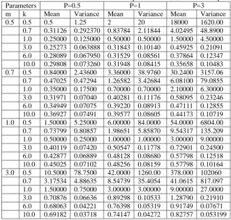
Table 1 shows the mean and the variance of p-k gamma distribution for λ = 1 and different values of parameters m, p, and k.

Table-1: Mean and variance for different values of the three parameters m, k, and m of the p-k Gamma model

Parameters P=0.5 P=1 P=3

m k Mean Variance Mean Variance Mean Variance

0.5 0.5 0.5 1.25 2 20 18000 1620.00

0.7 0.31126 0.292370 0.83784 2.11844 4.02495 48.8900 1.0 0.25000 0.125000 0.50000 0.50000 1.50000 4.50000 3.0 0.25273 0.063888 0.31843 0.10140 0.45925 0.21091 6.0 0.28089 0.067950 0.31529 0.08561 0.37864 0.12347 10.0 0.29808 0.073260 0.31948 0.08415 0.35658 0.10483 0.7 0.5 0.84000 2.43600 3.36000 38.9760 30.2400 3157.06 0.7 0.47025 0.47294 1.26582 3.42684 6.08100 79.0855 1.0 0.35000 0.17500 0.70000 0.70000 2.10000 6.30000 3.0 0.31971 0.07040 0.40281 0.11176 0.58095 0.23246 6.0 0.34949 0.07075 0.39220 0.08913 0.47111 0.12855 10.0 0.36927 0.07491 0.39577 0.08605 0.44173 0.10719 1.0 0.5 1.50000 5.25000 6.00000 84.0000 54.0000 6804.00 0.7 0.73799 0.80857 1.98651 5.85870 9.54317 135.209 1.0 0.50000 0.25000 1.00000 1.00000 3.00000 9.00000 3.0 0.40119 0.07420 0.50547 0.11778 0.72901 0.24500 6.0 0.42877 0.06889 0.48128 0.08680 0.57798 0.12518 10.0 0.45025 0.07102 0.48256 0.08159 0.57798 0.10164 3.0 0.5 10.5000 78.7500 42.0000 1260.00 378.000 102060

0.7 3.17534 4.88635 8.54739 35.4054 41.0615 817.097 1.0 1.50000 0.75000 3.00000 3.00000 9.00000 27.0000 3.0 0.70876 0.06636 0.89298 0.10533 1.28790 0.21910 6.0 0.68063 0.04221 0.76398 0.05319 0.91749 0.07671 10.0 0.69182 0.03718 0.74147 0.04272 0.82757 0.053199

One can notice that for fixed values of m and k, and p ≥ 1 the mean and the variance are decreasing functions of k. For fixed m (m < 1) and p (p < 1), the mean and the variance first decrease (k ≤ 1) then increases as k increases (k < 1). The mean and the variance are increasing functions of p when m and k are fixed. Also, the mean and the variance are increasing functions of m when k and p are fixed.

Table-2: Skewness and Kurtosis for different values of the three parameters m, k, and m of the p-k Gamma model

Parameters p=0.5 p=1 p=3

m k Skewness Kurtosis Skewness Kurtosis Skewness Kurtosis 0.5 0.5 6.61876 84.7200 6.61876 84.7200 6.61876 84.7200

0.7 4.18245 29.5209 4.18245 29.5209 4.18245 29.5209 1.0 2.82843 12.0000 2.82843 12.0000 2.82843 12.0000 3.0 1.16211 0.83789 1.16211 0.83789 1.16211 0.83789 6.0 0.82333 -0.32380 0.82333 -0.32380 0.82333 -0.32380 10.0 0.71749 -0.63487 0.71749 -0.63487 0.71749 -0.63487 0.7 0.5 5.36870 54.7027 5.36870 54.7027 5.36870 54.7027

0.7 3.49837 20.5420 3.49837 20.5420 3.49837 20.5420 1.0 2.39046 8.57143 2.39046 8.57143 2.39046 8.57143 3.0 0.88141 0.20896 0.88141 0.20896 0.88141 0.20896 6.0 0.52782 -0.71982 0.52782 -0.71982 0.52782 -0.71982 10.0 0.40994 -0.97092 0.40994 -0.97092 0.40994 -0.97092 1.0 0.5 4.30201 34.4082 4.30201 34.4082 4.30201 34.4082

0.7 2.89489 13.9844 2.89489 13.9844 2.89489 13.9844 1.0 2.00000 6.00000 2.00000 6.00000 2.00000 6.00000 3.0 0.63278 -0.15848 0.63278 -0.15848 0.63278 -0.15848 6.0 0.25310 -0.86963 0.25310 -0.86963 0.25310 -0.86963 10.0 0.114609 -1.05757 0.114609 -1.05757 0.114609 -1.05757 3.0 0.5 2.23121 8.76571 2.23121 8.76571 2.23121 8.76571

0.7 1.62537 4.34224 1.62537 4.34224 1.62537 4.34224 1.0 1.15470 2.00000 1.15470 2.00000 1.15470 2.00000 3.0 0.16810 -0.27054 0.16810 -0.27054 0.16810 -0.27054 6.0 0.29480 -0.33438 0.29480 -0.33438 0.29480 -0.33438 10.0 0.54854 -0.18327 0.54854 -0.18327 0.54854 -0.18327

The Moment Generating Function of p-k gamma distribution

Here, we will obtain the moment generating function of the new distribution as follows:

𝐸(𝑒𝑡𝑥₎

= _Г𝜆−𝑚

𝑘

𝑝 (𝑚)� 𝑥

𝑚−1_𝑒−((𝑥/𝜆)

𝑘

𝑝 −𝑡𝑥) ∞

0 𝑑𝑥

=�𝜆𝑖𝑡𝑖_𝑖!𝑝Г_Г𝑘(𝑚+𝑖) 𝑘 𝑝 (𝑚) ∞

𝑖=0

(36)

=�𝜆𝑖𝑡𝑖(𝑝/_𝑖!𝑘_Г)𝑖Г𝑘(𝑚+𝑖) 𝑘(𝑚) ∞

𝑖=0

(37)

=�𝜆𝑖𝑡𝑖(𝑝)_𝑖𝑖/_!𝑘_ГГ₍((_𝑚𝑚_/𝑘+₎ 𝑖)/𝑘) ∞

𝑖=0

(38)

Differentiating (36-38) r th times with respect to t and putting t equal to zero, we will obtain the r th moment of p-k gamma distribution.

Shannon’s Entropy

To measure variation of uncertainty, Shannon in 1948 defined the entropy of a random variable X to be

𝜂𝑋 =𝐸[−𝑙𝑛𝑓(𝑥)]. Entropy has various applications in many fields such as science, engineering, and economics.

Using (2), we get the following form of Shannon’s entropy of p-k gamma:

𝜂𝑋 _{=𝐸[−ln (} 𝜆−𝑚 Г𝑘 𝑝 (𝑚)𝑥

𝑚−1_𝑒−(𝑥/𝜆)𝑘/𝑝_)]

=𝐸[𝑚𝑙𝑛(𝜆) + ln� Г𝑝 𝑘(𝑚)� −(𝑚 −1) ln(𝑥) + (𝑥/𝜆)𝑘/𝑝]

=𝑚𝑙𝑛(𝜆) + ln (𝑝Г𝑘(𝑚))−(𝑚 −1)𝐸[ln(𝑥)] +𝐸[(𝑥/𝜆)𝑘/𝑝]

To compute 𝐸[ln(𝑥)], we first compute 𝐸(𝑥𝑤) and differentiate it with respect to w then put 𝑤= 0 . i.e. we have

𝜂𝑋 =𝑚𝑙𝑛(𝜆) + 𝑝Г𝑘(𝑚)−(𝑚 −1)𝑝𝜓𝑘(𝑚) +𝐸[(𝑥/𝜆)𝑘/𝑝]

=𝑚𝑙𝑛(𝜆) + 𝑝Г𝑘(𝑚)−(𝑚 −1)𝑝𝜓𝑘(𝑚) +_𝑘𝑝𝑚� Г𝑝 𝑘(𝑚)�.

(40)

For λ = 1 and p=k, we have Shannon’s entropy of k-gamma distribution with parameters m and k and for p=k=1, we

have Shannon’s entropy of gamma distribution with parameters m and λ.

Functions of p-k Gamma Random Variables

If X and Y are independent, have p-k gamma distributions with pdfs given by (28) then (𝑥/𝜆)𝑘+ (𝑦/𝜆)𝑘/𝑝 has a gamma distribution (𝑛+𝑚

𝑘 ,𝑝).

If X and Y are independent, have p-k gamma distributions with pdfs given by (28) then (𝑥/𝜆)𝑘

(𝑥/𝜆)𝑘_+(𝑦/𝜆)𝑘 has a p-k beta

distribution with pdf 𝑓(𝑧) = 1

𝑘 |𝑝𝐵𝑘(𝑚,𝑛)𝑧 𝑚

𝑘−1(1− 𝑧)𝑛𝑘−1or has 1

𝑘 Beta distribution( m/ k,n/ k).

3.1 Maximum Likelihood Estimation

Let x1, x2, ..., xn be a random sample of size n follows p-k gamma distribution. To estimate the four unknown parameters (p, k, m, λ) of the new distribution we obtain the likelihood function with the form:

𝐿=∏ 𝜆_Г−𝑚

𝑘 𝑝 (𝑚)

𝑛

𝑖=1 ∏𝑛𝑖=1(𝑥𝑖𝑚−1)∏ 𝑒𝑛𝑖=1 −(𝑥𝑖/𝜆)𝑘/𝑝, (41)

Taking the logarithm- of likelihood function, we get

𝑙𝑛𝐿=−𝑚𝑙𝑛[𝜆]− 𝑛𝑙𝑛� Г𝑝 𝑘(𝑚)�+ (𝑚 −1)∑𝑛𝑖=1ln [𝑥𝑖]− ∑ (𝑥𝑖/𝜆)

𝑘

𝑝 . 𝑛

𝑖=1 (42)

The first derivatives of the log-likelihood function are given as follows

𝜕𝑙𝑛𝐿

𝜕𝑚 =−𝑛 𝜓𝑝 𝑘(𝑚) +�ln[𝑥𝑖] 𝑛

𝑖=1

,

𝜕𝑙𝑛𝐿

𝜕𝑝 =−𝑛𝑚_𝑘𝑝+�(𝑥𝑖/𝜆) 𝑘 𝑝2 𝑛 𝑖=1 , (43) 𝜕𝑙𝑛𝐿

𝜕𝑘 =𝑛(1

𝑘+ 𝑚

𝑘2(ln[𝑝] +𝜓 � 𝑚

𝑘�))− � �𝑥𝑖 𝜆 � 𝑘 𝑝 𝑛 𝑖=1

ln[𝑥𝑖], 𝜕𝑙𝑛𝐿

𝜕𝜆 ₌₋𝑛 𝜆+�

𝑘 𝜆 �𝑥𝑖 𝜆 � 𝑘 𝑝 𝑛 𝑖=1 .

where ψ(.) the logarithmic derivative of gamma function is known as Psi function (digamma function).

Equating (43) to zero and solving them numerically, one can obtain the estimates of the unknown parameters. Now, the second order derivative of log-likelihood function are obtained as follows

𝜕2_𝑙𝑛𝐿

𝜕𝑛2 =−𝑛 𝜓′𝑝 𝑘(𝑚) =− 𝑛 𝑘2 𝜓′ �

𝑚

𝑘�=−𝑛𝑘𝜁𝑘(𝑚, 2), 𝜕2_𝑙𝑛𝐿

𝜕𝑛𝑘 =𝑛𝑘

2_{(𝑚𝑙𝑛[𝑝] +𝑚𝜓(}𝑚 𝑘)), 𝜕2_𝑙𝑛𝐿

𝜕𝑚𝑝 =− 𝑛𝑚

𝑝𝑘, 𝜕2_𝑙𝑛𝐿

𝜕𝑝2 = 𝑛𝑚

𝑘2_{𝑝 −}2� � 𝑥𝑖

𝜆� 𝑘

/𝑝3_, 𝑛

𝑖=1 𝜕2_𝑙𝑛𝐿

𝜕𝑝𝑘 =_𝑘𝑛𝑚2_𝑝+� 𝑥𝑖𝑘/𝑝2ln [𝑥𝑖], 𝑛

𝑖=1 𝜕2_𝑙𝑛𝐿

𝜕2_𝑙𝑛𝐿

𝜕𝑘2 =−𝑛(−2_𝑘𝑚₃ln[𝑝] +_𝑘1₂+ 2_𝑘𝑚₃𝜓 �𝑚_𝑘� −𝑚 2 𝑘4𝜓′ �

𝑚 𝑘� −

1

𝑝 � � 𝑥𝑖

𝜆� 𝑘

ln [𝑥𝑖]), 𝑛

𝑖=1

(44)

𝜕2_𝑙𝑛𝐿

𝜕𝑘𝑚 =𝑛(

ln[𝑝]

𝑘2 +

1

𝑘2𝜓 � 𝑥 𝑘�), 𝜕2_𝑙𝑛𝐿

𝜕𝑘𝑝 =_𝑝𝑘𝑛𝑚2− � � 𝑥𝑖

𝜆� 𝑘

/𝑝2_{ln [𝑥} 𝑖]), 𝑛

𝑖=1 𝜕2_𝑙𝑛𝐿

𝜕𝑝𝜆 =−𝑛_𝜆+𝑘_𝜆� �𝑥_𝜆𝑖� 𝑘

/𝑝2_, 𝑛

𝑖=1 𝜕2_𝑙𝑛𝐿

𝜕𝑘𝜆 =𝑘_𝜆+� �𝑥_𝜆𝑖� 𝑘

/𝑝𝑙𝑛[𝑥𝑖] + 𝑛

𝑖=1

� �𝑥_𝜆𝑖�𝑘/𝑝,

𝑛

𝑖=1 𝜕2_𝑙𝑛𝐿

𝜕𝜆2 ₌ 𝑛 𝜆2+

𝑘(𝑘+ 1)

𝜆2 � �𝑥𝑖 𝜆 � 𝑘 𝑝 . 𝑛 𝑖=1

where 𝜓′(. ) the first derivative of Psi function and 𝜓(𝑛)(. ) the nth derivative of Psi function which is known as PolyGamma and 𝜁_𝑘(. , . ) k-Zeta function defined by 𝜁_𝑘(𝑚,𝑟) =∑∞_{𝑖=1(𝑥+𝑛𝑘}1 _)𝑟. and the information matrix is given by

𝐽(𝜃) =−

⎣ ⎢ ⎢ ⎢ ⎡

𝐼𝑚,𝑚 𝐼𝑚,𝑝 𝐼𝑚,𝑘 𝐼𝑚,𝜆 𝐼𝑝,𝑚 𝐼𝑝,𝑝 𝐼𝑝,𝑘 𝐼𝑝,𝑘 𝐼𝑘,𝑚 𝐼𝑘,𝑝 𝐼𝑘,𝑘 𝐼𝑘,𝜆

𝐼𝜆,𝑚 𝐼𝜆,𝑝 𝐼𝜆,𝑘 𝐼𝜆,𝜆 ⎦ ⎥ ⎥ ⎥ ⎤

(45)

where 𝐼 is the expected value of the second derivative of the log-likelihood with respect to the parameters. Inverting the information matrix and replacing the unknown parameters by their mles to obtain the asymptoticvariance-covariance matrix of (𝑚�, 𝑝̂, 𝑘�,𝜆�). 100(1−γ) % approximate confidence intervals for the parameters m, p, k and λ are respectively,

�𝑚�±𝑧𝛾

2�𝑣𝑎𝑟(𝑚�)�, �𝑝̂±𝑧𝛾

2�𝑣𝑎𝑟(𝑝̂)�, �𝑘�±𝑧𝛾

2�𝑣𝑎𝑟�𝑘���,𝑎𝑛𝑑

(𝜆̂±𝑧𝛾

2�𝑣𝑎𝑟(𝜆̂)).

3.2 Numerical Study

Now, we generate 1000 random samples of p-k gamma distribution with size 50 to study the behavior of the mle via absolute value of relative bias (ARbias) and scaled root mean square error (SRmse). With different actual values of the four parameters one can note that the ARbias and the SRmse for λ decreases when λ < 1 than for λ > 1. For k (with m, p, and λ < 1), the ARbias decreases when k > 1 than k < 1 while the SRmse increases for k > 1 than k < 1 and vise verse when m, p, and λ > 1. For m (if k, p, and λ < 1) the ARbias and SRmse increases for m > 1 than m < 1 but if k, p, and λ

> 1 the ARbias increases but the SRmse decreases for m > 1. For p m, k, and λ < 1 the ARbias and the SRmse increase

for p > 1 than p < 1 but if k, p, and λ < 1 the ARbias and the SRmse decrease for p > 1.

Table-3: MLEs, RAbias and SRmse of the four unknown parameters of the p-k gamma distribution for various values of the parameters at sample size = 50

Actual value m k p λ

m, k, p, λ Mean

RAbias

0.5 0.5 0.5 1.5 1.164560 0.437730 0.428467 0.774653 0.5 0.5 0.5 0.5 0.929414 0.414589 0.507859 0.271593 3.5 1.5 1.5 1.5 0.695548 0.598289 0.637259 0.521955 1.5 0.5 0.5 0.5 1.172330 0.829790 0.643199 0.016539 0.5 1.5 0.5 0.5 0.081051 0.153065 0.180960 0.122607 0.5 0.5 1.5 0.5 1.388080 0.343319 0.730883 0.003266 3.0 3.0 0.5 0.5 0.236092 0.861186 0.142704 0.702721 3.0 3.0 3.0 0.5 0.321226 0.806608 0.926590 0.019895 3.0 3.0 3.0 3.0 0.716855 0.737184 0.533468 0.623053

SRmse

0.5 0.5 0.5 1.5 1.636170 0.533277 0.570789 0.778332 0.5 0.5 0.5 0.5 1.363130 0.501656 0.615331 0.377077 3.5 1.5 1.5 1.5 0.935574 1.019900 0.664488 0.653378 1.5 0.5 0.5 0.5 1.566090 0.832005 0.679550 0.400326 0.5 1.5 0.5 0.5 0.578083 2.522110 1.146430 1.234466 0.5 0.5 1.5 0.5 1.625490 0.445592 0.764855 0.938695 3.0 3.0 0.5 0.5 0.788617 0.863460 0.393248 0.773012 3.0 3.0 3.0 0.5 0.788199 0.810226 0.987246 0.746850 3.0 3.0 3.0 3.0 0.718401 0.740945 0.578034 0.636148

4. SUMMARY

In this paper we introduced a new distribution via two parameter gamma function called p-k gamma function. Some properties of the new distribution are derived and estimation of unknown parameters is discussed.

REFERENCES

1. G. E. Andrews, R. Askey and R. Roy (1999). Special Functions, Cambridge University Press.

2. R. Diaz and E. Pariguan (2017). On Hypergeometric Functions and Pohchammer k-Symbol, Divulgaciones Mathematicas, 15(2): 179-192.

3. K. S. Gehlot, (2017). Two Parameter Gamma Function and It’s Properties, https: //arxiv.org/pdf/1701.01052, 11-Nov-2018.

4. S. Mubeen, N. Sadiq and F. Shaheen, Properties of k-gamma, k-beta and k-psi functions. Bothalia Journal, 4(2014): 371-379. 13

5. G. Rahman, S. Mubeen, A. Rehman and M. Naz, (2014). On k-Gamma and k-Beta Distributions and Moment Generating Functions, Journal of Probability and Statistics, Volume 2014, Article ID 982013, 6 pages. 6. E. D. Rainvile (1960). Special Functions. the Macmillan, New York, USA.

7. N. M. Temme (1996). Special Functions: An Introduction to the Classical Functions of Mathematical Physics, John Wiley and Sons, Inc.

Source of support: Nil, Conflict of interest: None Declared.