AUSTRALIAN JOURNAL OF BASIC AND
APPLIED SCIENCES
ISSN:1991-8178 EISSN: 2309-8414 Journal home page: www.ajbasweb.com
Open Access Journal
Published BY AENSI Publication
© 2016 AENSI Publisher All rights reserved
This work is licensed under the Creative Commons Attribution International License (CC BY).
http://creativecommons.org/licenses/by/4.0/
To Cite This Article: S. Karthikeyan, M.C. Pravin, B. Sathyabama and M. Mareeswari., DWT Based LCP Features for the Classification of Steel Surface Defects in SEM Images with KNN Classifier. Aust. J. Basic & Appl. Sci., 10(5): 13-19, 2016
DWT Based LCP Features for the Classification of Steel Surface Defects in
SEM Images with KNN Classifier
1
S. Karthikeyan, 2M.C. Pravin, 3B. Sathyabama and 4M. Mareeswari
1
Assistant Professor, Thiagarajar College of Engineering, Mechanical Engineering, Madurai, India.
2Research Scholar, Thiagarajar College of Engineering, Mechanical Engineering, Madurai, India
3Associate Professor, Thiagarajar College of Engineering, Electronics and Communication Engineering, Madurai, India. 4Project fellow, Thiagarajar College of Engineering, Mechanical Engineering, Madurai, India
Address For Correspondence:
M.C. Pravin, Research Scholar, Thiagarajar College of Engineering, Mechanical Engineering, Madurai, India Tel: 9789715050 E-mail: [email protected])
A R T I C L E I N F O A B S T R A C T
Article history:
Received 12 January 2016 Accepted 22 February 2016 Available online 1 March 2016
Keywords:
Scanning Electron Microscope Surface quality Discrete Wavelet Transform Local Configuration Pattern (LCP) KNN Classifier
This paper presents a Texture based approach for detecting and characterizing defects on steel surfaces, through which the quality inspection of steel products is performed. Our objective is to detect the defects in the surface of steel products. Major defects like corrosion, crack, scratch and fracture are considered for testing and training process. The Discrete Wavelet Transform (DWT) based Local Configuration Pattern (LCP) features are given as input to the KNN classifier. In order to explore multichannel discriminative information of both the microscopic configuration and local structures, DWT based LCP which is a combination of Local Binary Pattern (LBP) and Microscopic Configuration modeling (MiC) method is proposed. LCP and Defect Severity Index values are calculated for the sub-images obtained after applying DWT. The overall accuracy of DWT based LCP method is 96.7%. The results show that the proposed method produces better classification accuracy when compared to the classical methods.
INTRODUCTION
formed on the material surface. Surface texture can be defined as typical surface of a material, including geometric irregularities in or the composite of certain deviations. It includes roughness, waviness, lay (grain), etc. This paper aims at developing texture based recognition of steel surface defects using SEM images. Texture based methods will give a clear representation to analyse this surface defects (Yimo Guo, 2011). The paper is organized as follows. Section 1 explains the proposed methodology; Section 2 discusses the experimental results and Section 3 conclusion and future research.
1. Methodology:
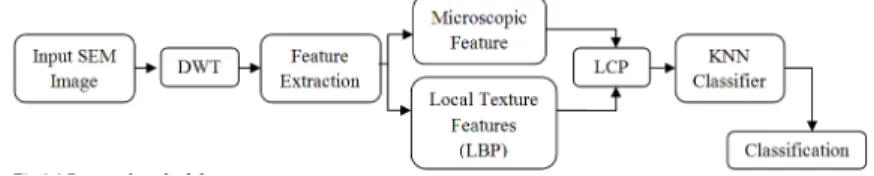
Figure 1.1 shows the proposed defect classification methodology. Initially DWT is applied to the input image to analyze the defects at multi scale level and the resultant sub-images are calculated for Local Configuration Pattern value. LCP combines the local structural information and Microscopic configuration information. The LCP feature vector is given as input for KNN classifier to categorize the defect. It is used to measure the Defect Severity Index (DSI). The aim of calculating this parameter is to provide a direct measurement of the quality of the product specifically reliability, fault tolerance and stability.
Fig. 1.1: Proposed methodology.
A. GLCM features:
In statistical texture analysis, texture features are computed from the statistical distribution of observed combinations of intensities at specified positions relative to each other in the image. The Gray Level Co-occurrence Matrix (GLCM) technique is a method of extracting second order statistical texture features. Some of these measures related to the specific texture characteristics of the image such as homogeneity, contrast, energy and the presence of organized structure within the image.
B. Tamura features:
The Tamura features, including coarseness, contrast, directionality, line likeness, regularity, and roughness, are designed in accordance with psychological studies on the human perception of texture. Coarseness, contrast and directionality are essential factors in texture and have high potential to distinguish different textures. All of them were measured by human subjects.
C. Laws mask:
Laws identified the following properties as playing an major role in describing texture uniformity, density, coarseness, directionality, roughness, regularity, linearity, direction, frequency, and phase. Laws texture energy measures determine texture properties by assessing Edges, Spots, Average Gray Level, Ripples and Waves in texture. The measures are derived from three simple vectors. E3 = (-1, 0, 1) calculating first difference (edges), L3 = (1, 2, 3) which represents averaging, and S3 = (-1, 2, -1) corresponding to the second difference (spots).
D. Local Configuration Pattern (LCP):
LCP feature decomposes the information architecture of images into two levels, as (1) local structural information; (2) microscopic configuration information that involves image configuration and pixel-wise interaction relationships. For local structural information, LBP is used in feature extraction framework, whereas a microscopic configuration model is developed to explore microscopic configuration information.
(i) Local Binary Pattern (LBP):
LBP is defined as an ordered set of binary comparisons of pixel intensities between the center pixel and its eight surrounding pixels (Yimo Guo, 2011). The decimal form of the resultant 8-bit word (LBP code) can be expressed as follows.
∑
=−
=
70
(
)
2
)
,
(
x
cy
c ns
i
ni
c nLBP
(1)
Where ic corresponds to the gray value of the center pixel (xc, yc), in to the gray values of the 8 surrounding pixels, and function s(x) is defined as:
< ≥ =
0 0
0 1
) (
x if
x if x
S
The LBP8 operator produces 256 (28) different output values, corresponding to the 256 different binary patterns. To remove the effect of rotation, i.e., to assign a unique identifier to each rotation invariant LBP, a circular bit-wise right shift operator is performed on the pattern to obtain minimal number of transitions.
7 , 1 , 0 )) , ( min( 8
8 = ROR LBP i i= KK LBPri
(3)
(ii) Modeling of Microscopic Configuration (MiC):
To model the image configuration with respect to each pattern, optimal weights associating with intensities of neighboring pixels are estimated, to linearly reconstruct the central pixel intensity [6]. This can be expressed by:
∑
− = − = − ∗ 1 0 10... )
(
P
i i i
c
P
g
a
g
a
a
E
(4)
gc, gi are intensity values
(
i = 0;... p −1)
ai are weighting parameters
− = 1 , . . 1 , 0 , L L L L L N C C C C (5)
The intensities of their neighboring pixels Vi;0…., Vi;p-1 (i=0,….NL-1) can thus be organized as
− − − − − − = 1 ; 1 ... 1 ; 1 0 ; 1 . 1 ; ... 1 ; 0 ; 1 ; ... 1 ; 0 ; 1 1 1 0 0 0 P VN VN VN P V V V P V V V V L L L L (6)
In order to minimize the reconstruction error in eqn (6), the unknown parameters ai (i=0,…, P-1) are constructed as a column vector:
− = 1 . . 1 0 ap a a AL (7)
In this way, the problem to be solved becomes a least-squares problem CL=ALVL. When the system is over-determined, optimal parameter vector AL is determined by:
(
)
LT L L T L
L V V V C
A = −1 (8)
In texture analysis, rotation invariant analysis is a widely studied problem, aims at providing texture features that are invariant to rotation angle of the input image. To produce rotation invariant features, 1D Fourier transform is applied to the estimated parameter vector AL. The transformed vector can be expressed by:
P Ki j P i L
L K
A
i eh
2 /1 0 ) ( ) ( − ∏ − = ∗ =
∑
(9) Where hx (k) is the Kth element of hx and AL (i) is the ith element of AL. Although image rotation would leadto cyclic translations of AL, Fourier transform is invariant to this kind of translations so that hx could achieve rotation invariant property. The magnitude part of vector hL is taken as the MiC feature, which is defined by:
−
=
h
(0);h
(1);... ...h
(P 1)h
k L L L (10)Considering that hL encodes the image configuration and pixel-wise interaction relationship of each specific pattern, it together along with pattern occurrences of local binary patterns would construct a complementary feature for both the discrimination of microscopic configuration and local structures .The final feature is
[
] [
]
[
]
[
; ; ; ;... ;]
; 1 1 1 1 00
o
h
o
h
o
h
q qLCP = − −
(11)
Where hL is calculated by Equation (10) with respect to the ith pattern of interest, Oi is the occurrence of the ith local pattern of interest (i.e., the LBP), and q is the total number of patterns of interest. Moreover, multi-scale analysis can be achieved by constructing LCPs for different decomposed level of input image by wavelet transforms.
E. KNN classifier:
K-Nearest Neighbor (KNN) is one of the most popular algorithms for pattern recognition. The classification rules are generated by the training samples themselves without any additional data. The KNN classification algorithm forecast the test sample’s category according to the K training samples which are the nearest neighbors to the test sample, and judge it to that category which has the largest category probability [9]. The process of KNN algorithm to classify example X is:
• Suppose there are j training categories C1,C2,…,Cj and the sum of the training samples is N after feature reduction, they become m-dimensional feature vector.
• Make sample X to be the same feature vector of the form (X1, X2…, Xm), as all training samples.
• Calculate the similarities between all the training samples and X. Taking the ith sample di (di1,di2,…,dim) as an example, the similarity SIM(X, di) is as follows,
2
1 2
1 1
. )
, (
=
∑
∑
∑
= =
=
m
j ij m
j j m
j ij j
i
d
X
d
X
d X SIM
(12)
• Choose k samples which are larger from N similarities of SIM(X, di), (i=1, 2…, N), and treat them as a KNN collection of X. Then, at last calculate the probability of X belong to each category respectively with the following formula.
∑
=
d
j i i
j
SIM
X
d
y
d
C
C
X
P
(
,
)
(
,
).
(
,
)
(13)
∉ ∈ =
j i
j i
j i
C d
C d C d y
0 , 1 ) , (
(14)
Where y (di,Cj) is a category attribute function.
Judge sample X to be the category which has the largest P (X, Cj).
RESULTS AND DISCUSSIONS
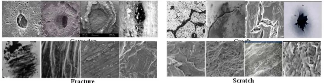
Experiments have been conducted to calculate the performance of the proposed method using the 156 SEM images of steel collected from various web resources. It includes various steel defects like scratch (29), corrosion (40), fracture (23), hole (25) and crack (39). (.) shows the number of images in each type. In that 5 images from each type with a single rotation i.e. a total of 50 images are considered for training and 350 images (which include 156 original images and its distorted versions) are used for testing. Some of the samples (Corrosion, Crack, Fracture and Scratch) from the formed dataset are shown in Fig.2.1
A. Data Set:
Fig. 2.1: Sample SEM images of Steel defects.
B. Wavelet Decomposition:
The texture energy is stored in different frequencies for different types of defects. An example is shown in Fig 2.2 Thus, instead of extracting the features on the original image, it is extracted in different frequency components (LL, LH, HL, HH) of the image. The maximum value of features in LL, LH, HL and HH is considered as the representative feature value.
C. LCP & defect severity index:
Severity Index (DSI). This parameter determines the quality of the product, based on which one can take decision for releasing the product i.e. it indicates the product quality. The DSI is defined as
defect of no total
vel severityle defect
DSI
_ _ _
*
∑
=
(15)
Fig. 2.2: Wavelet Decomposition of Defects.
D. Classification Results:
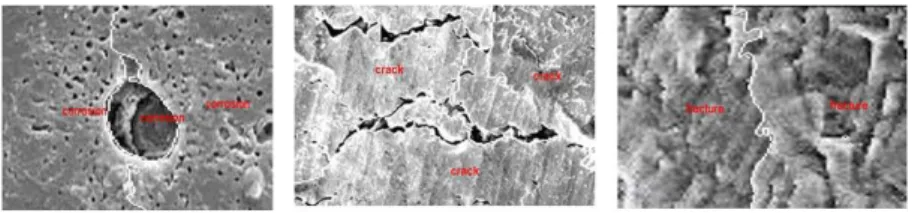
Fig 2.3: Classification of various defects from left to right corrosion, crack and fracture.
To calculate the Defect Severity Index (DSI) the LCP magnitude is grouped into minor, medium, major and critical. Weights are assigned to each severity level. This varies for different types of defects. To achieve this minimum and maximum values of LCPs each training set are spitted into four bins and each bin is assigned with a weight after defect detection the DSI value is calculated using eqn (13). Table 2.1 shows the DSI and LCP values taken for the sub-images of input SEM corrosion image.
The LCP values for LL, LH, HL and HH sub-images are tabulated. It is inferred that HH sub-image for all the images have been obtained highest LCP value and also the severity index value. The HH sub-image has the high frequency components which obviously detect the defective part. In trial and error method, DSI value is high for fully corroded images. Therefore corrosion defect falls under the critical severity level. The priority level for this severity is to resolve immediately and Table 2.2 shows the DSI for crack images. HL sub-images for all the images have been obtained highest LCP value and also the severity index value.
Therefore crack defect falls under the major severity level. Table 2.3 shows the DSI for scratch images. In this table, HL sub-images for all the images have been obtained highest LCP value and also the severity index value. Table 2.4 shows the DSI for fracture images. It is inferred that LH sub-images for all the images have been obtained highest LCP value and also the severity index value. Therefore fracture defect falls under the medium severity level. The LCP values for LL, LH, HL and HH sub-images are given to the KNN classifier. The various defects were classified using KNN classifier as shown in Figure 2.3. The performance of the KNN classifier for different methods like GLCM, Tamura, Laws mask, and DWT-LCP are discussed below.
Table 2.1: LCP and DSI Computation of corrosion image.
IMAGE HH DSI HL DSI LH DSI LL DSI
0.987 8.41e+0 0.139 0.029 2.08 0.005 0.008 430.7
32.211 647.16 1.301 0.1606 15.856 16.14 1.071 0.329
43.904 177.31 23.74 4.855 0.245 0.035 0.389 0.002
0.65 1.5e003 0.053 2.834 0.007 4.3e-06 0.292 0.52
E.Performance Analysis:
Table 2.2: LCP and DSI Computation of crack image.
IMAGE HH DSI HL DSI LH DSI LL DSI
17.89 0.0081 0.350 1.5e5 3.711 0.0252 0.099 3.244
75.88 0.0047 7.653 422.98 2.333 0.0095 0.016 85.509
53.03 0.0022 0.068 0.628 0.018 0.0054 0.003 5.3e-3
293.4 0.0187 28.99 1.184e3 28.16 0.0033 0.089 6.018
Table 2.3: LCP and DSI Computation of scratch image.
IMAGE HH DSI HL DSI LH DSI LL DSI
952.76 1.5e-6 250.24 1.8e29 35.84 5.9e-3 0.0643 2.8e3
44.282 5.4e-3 0.9653 265.15 2.2528 0.0075 0.0059 0.0187
42.928 4.7e-4 0.0787 1.07e3 7.2006 0.0014 0.0056 0.0066
252.53 0.0022 21.841 1.57e4 26.089 0.0609 0.127 997.77
Table 2.4: LCP and DSI Computation of fracture image
IMAGE HH DSI HL DSI LH DSI LL DSI
0.875 0.056 0.203 0.2476 0.2021 2.966 0.0191 2.3e-003
18.196 0.0022 0.7481 0.2741 1.6963 1.9985 0.052 0.057
19.227 0.0071 0.0314 11.473 0.7386 20.152 0.002 18.516
84.14 1.8e-3 21.8 6.3e-31 41.908 0.0187 0.0117 2.4e-3
retrieved images no.of Total
retrieved images relevant No.of =
Precision (16)
retrieved images
relevant no.of
Total
retrieved images
relevant non No.of = rate
Error (17)
retrieved images no.of Total
retrieved images relevant No.of = Efficiency
Retrieval (18)
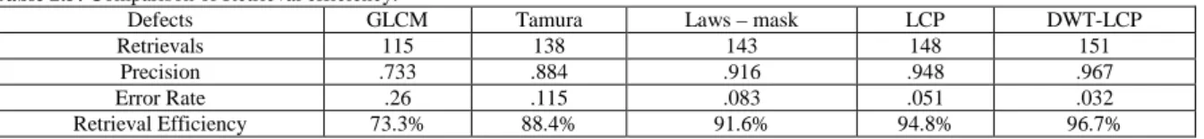
Table 2.5: Comparison of Retrieval efficiency.
Defects GLCM Tamura Laws – mask LCP DWT-LCP
Retrievals 115 138 143 148 151
Precision .733 .884 .916 .948 .967
Error Rate .26 .115 .083 .051 .032
Retrieval Efficiency 73.3% 88.4% 91.6% 94.8% 96.7%
images into level, ridge, wave, edge and line it can well discriminate cracks, corrosion and so on. This provides an accuracy of 91.6% & 94.8% for LCP which is comparatively high than Tamura and GLCM.
The SEM images provide a magnification view of surface defects which can be clearly separated by wavelet decomposition. Further LCP provides both the structural and micro level configuration information which improves the retrieval efficiency to 96.7%. The proposed method gives better results for all types of defect category which is shown in Table 2.5.
3. Conclusion:
In this paper, a DWT enabled LCP texture features have been developed for the classification of steel. The magnification of defects in SEM images provides an opportunity to analyse the steel surfaces at micro level. This can be directly computed using MiC and LBP. Further DWT has made the possibility of analysing the defects in various sub bands. The results obtained, indicate that the proposed method have better classification accuracy when compared with other methods by obtaining an overall accuracy of 96.7%. Thus classification of defects is possible with image analysis and may be used for correlating service/failure conditions based on morphology of the products.
ACKNOWLEDGMENT
Authors thank University Grants Commission (UGC) New Delhi and Departments of Mechanical Engineering, and Electronics and Communication Engineering, Thiagarajar College of Engineering, Madurai for support and assistance to carry out this work.
REFERENCES
Sathyabama, B., 2012. “Laws based quality inspection of steel products using scanning electron microscory images” International journal of computer applications, 25-29.
Jeffery Price, R., W. Kathy Hylton, W. Kenneth Tobin, Jr., R. Philip Bingham, D. John Hunn and R. John Haines, 2008. “Detection of cavitation pits on steel surfaces using SEM imagery,” 865: 574-5743.
Mike Muehlemann, 2000. “Standardizing Defect Detection for surface Inspection of Large Web Steel,” International Journal of Pattern Recognition and Artificial Intelligence, 735-755.
Son, I.H., J.D. Lee, S. Choi, D.L. Lee, Y.T. Im, 2008. “Deformation behavior of the surface defects of low carbon steel in wire rod rolling”, Journal of materials processing technology,” 201: 91–96.
Shigeru Takayaa and Kenzo Miyab, 2005. “Application of magnetic phenomena to analysis of stress corrosion cracking in welded part of stainless steel,”. Journal of Materials Processing Technology, 161: 66–74.
Kuldeep Agarwal, Rajiv Shivpuri, Yijun Zhu, Tzyy-Shuh Chang, Howard Huang, 2011. “Process knowledge based multi-class support vector classification approach for surface defects in hot rolling,”. Expert Systems with Applications, 38: 7251–7262.
Youngjoo Lee and Jeongjin Lee, 2014. “Accurate Automatic Defect Detection Method Using Quadtree Decomposition on SEM Images” IEEE Transactions on Semiconductor Manufacturing, 27-2.
Yimo Guo, Guoying Zhao, Matti pietik, 2011. “Texture classification using a linear configuration model based descriptor” Machine Vision Group, University of Oulu, Finland, BMVC.
Suguna, N. and Dr. K. Thanushkodi, 2010.” An improved KNN classification using genetic algorithm”, JCSI International Journal of Computer Science Issues, 7(4): 2.
Tamura and Mori, H., Yamawaki, 1978. Textural Features Corresponding to Visual Perception. IEEE Transaction on Systems, Man, and Cybernetcs, Vol. SMC-8, 6: 460–472.
Haralick, M., 1978. Statistical and structural approaches to texture. Proceedings of the IEEE, 67(5): 786– 804.