An Iterative Method for Solving the Matrix Equation X-A^{*}XA-B^{*}X^{-1}B=I

Mathematical and Software Engineering, Vol 6, No 1 (2020), 1–6. Varεpsilon Ltd, http://varepsilon.com/index.php/mse/

An Iterative Method for Solving the Matrix

Equation

_X

−

A

∗

XA

−

B

∗

X

−

1

B

=

I

Aynur Ali

_{and Vejdi Hasanov}

1

[email protected] Preslavsky University of Shumen, Faculty of Mathematics and Informatics, Shumen, Bulgaria

2_{[email protected] Konstantin Preslavsky University of Shumen, Faculty of Mathematics and}

Informatics, Shumen, Bulgaria

Abstract

In this paper we study iterative computing a positive definite solution of the matrix equation X−A∗XA−B∗X−1B = I. We propose an iterative method for finding a positive definite solution of the considered equation. The theoretical results are illustrated by numerical examples.

Subject ClassificationMSC: 15A24, 65F10, 65H10

Keywords: Matrix equation, Positive definite solution, Iterative methods

1

Introduction

We investigate the nonlinear matrix equation

X−A∗XA−B∗X−1B =I , (1) whereA, Baren×ncomplex matrices,I(orIn) is then×nidentity matrix, andA∗denotes

the conjugate transpose of A.

Eq. (1) has been introduced by Ali in [1], where an iterative method for computation a positive definite solution is proposed. A necessary and sufficient condition for the existence of a positive definite solution of Eq. (1) has been derived and a basic fixed point iteration has been proposed in [2]. In [3] by using the fixed point theorem for mixed monotone operator in a normal cone Gao has proved that the equation X −A∗_Xp_A−B∗_X−q_{B = I with}

0< p, q <1 always has the unique positive definite solution. In [4] the similar equation X−A∗XA+B∗X−1

B=I (2)

has been investigated. We interpret (1) and (2) as linearly perturbed equations of the well-known and studied equationsX−B∗X−1

B=I[5, 6] andX+B∗X−1

B=I[6, 7, 8, 9, 10], respectively.

In addition, there are some contributions in the literature to the solvability and numerical solutions of the matrix equationX+A∗X−1

A−B∗X−1

Motivated by [1, 2, 3, 4], we study Eq. (1) for finding a positive definite solution as propose an iterative method.

Throughout this paper, we denote byCn×n _{the set ofn×ncomplex matrices, by H}n

the set of n×n Hermitian matrices, by ρ(A) the spectral radius, by kAk the spectral norm kAk =pρ(A∗_{A). A > 0 (A ≥ 0) means that A is a Hermitian positive definite}

(semidefinite) matrix. If A−B > 0 (or A−B ≥ 0) we write A > B (or A ≥ B). For N ≥M >0 we use [M, N] to denote the set of matrices{X :M ≤X ≤N}.

2

Preliminaries

In this section we give some preliminary results.

In [1], the necessary conditions for existence of a positive definite solution and its lower bound have been obtained.

Theorem 1 [1, Theorem 2.1.] LetX be a positive definite solution of Eq. (1). Then

(a) ρ(A)<1, (b) ρ(X−1_B)

<1,

(c) X≥M, whereM is the unique positive definite solution of the equationX−A∗XA=I. In [2], it has been proven that ρ(A)<1 is a necessary and sufficient condition for the existence of a positive definite solution of Eq. (1). Moreover, it has been obtained an upper bound of all the solutions.

Theorem 2 [2, Theorem 2.] Eq. (1) has a positive definite solution X, if and only if ρ(A)<1. Moreover, the all positive definite solutions are in [M, N], where M and N are the unique solutions of the equations X −A∗_{XA = I and X −A}∗_{XA = I+B}∗_M−1_B, respectively.

Ali in [1] has investigated the iterative method

    

X0=I, Y0=βI, β >1

Xk+1=I+A∗XkA+B∗Y_k−1B, k= 0,1, . . .

Yk+1 =I+A∗YkA+B∗Xk−1B

(3)

for computing a positive definite solution of Eq. (1) based on the mixed monotone operator G(X, Y) = I+A∗_XA+B∗_Y−1

B. The sequences{Xk} and {Yk} defined by (3) have the following properties

X0≤X1≤ · · · ≤Xk ≤Yk≤ · · · ≤Y1≤Y0. (4) Moreover, it was proven that{Xk}and{Yk}withβ≥ ₁1+_−kkB_Ak_k22 converge to a unique positive

definite solution of Eq. (1) under conditionkAk2_+kBk2_<1.

In [2], it has been noted that the iterative method (3) can be used with X0 = M and Y0=N, where the matricesM andNare from Theorem 2. Moreover, it has been concluded that, if limk→∞kYk−Xkk= 0, then Eq. (1) has a unique positive definite solution.

Hasanov in [2] has considered the basic fixed point iteration (BFPI):

3

An iterative method

Here, we consider a modification of the iterative method (3), which is a partially inverse free variant.

LetM andN be the unique solutions of the equationsX−A∗XA=IandX−A∗XA= I+B∗M−1_{B, respectively. We consider}

        

X0=M, Y0=N, (orX0=I, Y0=βI), V0=Y0−1, Vk+1 =Vk(2I−YkVk),

Xk+1=I+A∗XkA+B∗Vk+1B, k= 0,1, . . . Yk+1 =I+A∗YkA+B∗X−

1

k B.

(6)

Lemma 1 [9, Lemma 3.2] Let C and P be Hermitian matrices of the same order and let P >0. Then CP C+P−1_≥2C.

Theorem 3 The sequences Vk,Xk andYk generated by iterative method (6) have the

fol-lowing properties

(i) X0≤X1≤. . .≤Xk≤Yk≤. . .≤Y1=Y0, k= 0,1, . . ., (ii) V0≤V1≤. . .≤Vk+1≤Y_k−1, k= 0,1, . . .,

(iii) limk→∞Xk = ¯X ≤Y¯ = limk→∞Yk, limk→∞Vk = ¯Y−1.

Proof. We prove the theorem by induction.

We haveX0=M ≤N =Y0 by Theorem 2. We compute V1=N−

1

(2I−N N−1) =N−1=V0,

X1=I+A∗M A+B∗V1B≥I+A∗M A=M =X0, Y1=I+A∗N A+B∗M−1B =N =Y0.

We have by Lemma 1 that

V1= 2V0−V0Y0V0≤Y0−1=N

−1

and

Y1−X1=A∗(N−M)A+B∗(M− 1

−V1)B≥B∗(M− 1

−N−1)B ≥0. Therefore,V0≤V1≤Y−

1

0 ,X0≤X1≤Y1≤Y0.

Assume thatVk−1≤Vk ≤Yk−−11 andXk−1≤Xk ≤Yk ≤Yk−1. Thus, we have Yk+1−Yk =A∗(Yk−Yk−1)A+B∗(X_k−1−X_k−₋11)B≤0, Vk+1−Vk =Vk(V_k−1−Yk)Vk ≥Vk(V_k−1−Yk−1)Vk≥0,

and

Xk+1−Xk=A∗(Xk−Xk−1)A+B∗(Vk+1−Vk)B≥0.

By Lemma 1, we have

Vk+1 = 2Vk−VkYkVk ≤Y_k−1.

Thus,

Yk+1−Xk+1=A∗(Yk−Xk)A+B∗(Xk−1−Vk+1)B

≥B∗(Y−1

k −Vk+1)B≥0. Hence, Xk ≤ Xk+1 ≤ Yk+1 ≤ Yk and Vk ≤ Vk+1 ≤ Y−

1

k for k = 1,2, . . .. Thus,

the limits limk→∞Xk, limk→∞Yk, and limk→∞Vk exist, and limk→∞Xk ≤ limk→∞Yk,

4

Numerical experiments

In this section we carry out numerical experiments for computing the positive definite solu-tion of Eq. (1) by iterative methods (3), (5), and (6) withX0=I,Y0=βI, andZ0= X0

+Y0

2 , where β = 1+kBk

2

1−kAk2 (or X0 =M,Y0 =N, where M and N are the unique solutions of the equationsX−A∗_XA=IandX−A∗_XA=I+B∗_M−1_{B, respectively).}

For the stopping criterion we take kYk−Xkk ≤ 10−10 for methods (3) and (6), and kZk −Zk−1k ≤ 10−10 for method (5), where k is the number of iterations. We use the notationres(X) =kX−A∗_XA−B∗_X−1_{B−Ik and compute}

• res(Xek) for methods (3) and (6), whereXek =Yk+₂Xk,

• res(Zk) for method (5).

Example 1 We consider Eq. (1) with

A= 1 56

   

1 5 3 2

−1 −6 3 4

−4 3 7 5

1 8 2 1

  

, B=

1 70    

7 9 6 8

7 5 8 3

9 8 6 7

11 5 9 3

   .

In Table 1 we report the results of experiment for Example 1 by using iterative methods (3), (5) and (6).

Table 1: Numerical results for Example 1.

Method k kYk−Xkk orkZk−Zk−1k res(Xek) orres(Zk)

byX0=IandY0=βI

(3) 11 8.8594e−11 4.5543e−13

(5) 10 4.0638e−12 4.3280e−11

(6) 12 1.4069e−11 3.0624e−14

byX0=M andY0=N

(3) 11 5.8609e−11 3.6315e−13

(5) 10 3.7103e−11 3.4837e−12

(6) 11 6.6076e−11 3.0991e−13

Example 2 We consider Eq. (1) with

A= 1 200      

41 15 23 35 66 25 12 27 45 21 23 27 28 16 24 15 45 16 52 65 66 21 24 65 35

     , B=

1 30      

23 21 23 25 32 21 45 60 42 33 23 24 34 18 17 13 42 18 44 30 32 33 26 30 26

     .

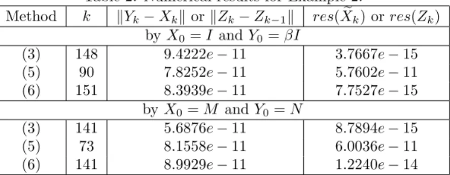
In Table 2 we report the results of experiment for Example 2 by using iterative methods (3), (5) and (6).

Acknowledgements

Table 2: Numerical results for Example 2.

Method k kYk−Xkkor kZk−Zk−1k res(Xek) orres(Zk)

byX0=IandY0=βI

(3) 148 9.4222e−11 3.7667e−15

(5) 90 7.8252e−11 5.7602e−11

(6) 151 8.3939e−11 7.7527e−15

byX0=M andY0=N

(3) 141 5.6876e−11 8.7894e−15

(5) 73 8.1558e−11 6.0036e−11

(6) 141 8.9929e−11 1.2240e−14

References

[1] A. Ali, For the matrix equation X −A∗_XA−B∗_X−1_{B = I, In: MATTEX 2018,} Conference proceeding, Vol. 1, 161-166, (2018). (in Bulgarian)

[2] V. Hasanov, Necessary and sufficient condition for the existence of a positive definite solution of a matrix equation, Annual of Konstantin Preslavsky University of Shumen, vol. XX C, pp. 13-19, (2019).

[3] D. Gao, Iterative methods for solving the nonlinear matrix equation X −A∗Xp_A−

B∗X−q_{B =I (0< p, q <1), Advances in Linear Algebra and Matrix Theory, 7, 72-78,}

(2017).

[4] V. Hasanov, Positive definite solutions of a linearly perturbed matrix equation, submitted [5] A. Ferrante, B. Levy, Hermitian solutions of the equation X = Q+N X−1

N∗, Linear Algebra Appl., 247, 359-373, (1996).

[6] C.-H. Guo, P. Lancaster, Iterative Solution of Two Matrix Equations, Math. Comput., 68, 1589-1603, (1999).

[7] W. N. Anderson, T. D. Morley, and G. E. Trapp, Positive Solution toX =A−BX−1_B∗_,

Linear Algebra Appl., 134, 53-62, (1990).

[8] J.C. Engwerda, A.C.M. Ran And A.L.Rijkeboer, Necessary and Sufficient Conditions for the Existence of a Positive Definite Solution of the Matrix EquationX+A∗X−1

A=Q, Linear Algebra Appl., 186, 255-275, (1993).

[9] XZ. Zhan Computing the extreme positive definite solutions of a matrix equation, SIAM J. Sci. Comput., 17, 632-645, (1996).

[10] B. Meini, Efficient computation of the extreme solutions of X+A∗X−1

A = Q and X−A∗X−1

A=Q, Math. Comput., 71, 1189-1204, (2001).

[11] M. Berzig, X. Duan, B. Samet, Positive definite solution of the matrix equationX =Q−

A∗_X−1_A+B∗_X−1_{B via Bhaskar-Lakshmikantham fixed point theorem, Mathematical} Sciences, 6, 27, (2012).

[13] A.A. Ali, V.I. Hasanov, On some sufficient conditions for the existence of a positive definite solution of the matrix equation X+A∗X−1

A−B∗X−1

B =I, In: Pasheva V, Popivanov N, Venkov G, editors, 41st International Conference Applications of Mathe-matics in Engineering and Economics AMEE 2015. AIP Conf. Proc. 1690, 060001 (2015), doi:10.1063/1.4936739.

[14] V. Hasanov, On the matrix equationX+A∗X−1

A−B∗X−1

B=I, Linear Multilinear A., 66, 1783-1798, (2018).

[15] A.C.R. Ran, M.C.B. Reurings, The symmetric linear matrix equation, Electron. J. Linear Al., 9, 93-107, (2002).

[16] P. Lancaster, M. Tismenetsky, The Theory of Matrices, 2nd ed. Academic Press, San Diego (CA), (1985).

[17] K. Deimling, Nonlinear functional analysis, Springer-Verlag, Berlin, (1985).