USING MULTI-FACET RASCH MODEL (MFRM) IN RATER-MEDIATED ASSESSMENT

UDC 811.111‟276.5:51 (535)

USING MULTI-FACET RASCH MODEL (MFRM)

IN RATER-MEDIATED ASSESSMENT

Farah Bahrouni

Sultan Qaboos University, Oman

Phone: +96899434899, E-Mail: bahrouni@squ.edu.om

Abstract. This paper is an introduction to the MFRM. It is intentionally meant to be simple with an attempt to avoid the sophisticated mathematical equations on which the calibration of the involved facets is based, wherever possible, so that little mathematical background does not obstruct the understanding. This paper aims at introducing the lay reader, who is involved in language performance assessment with no expertise, yet striving for objective assessment, to the Multi-Facet Rasch Model (MRFM) approach (Linacre, 1989). The reader will learn about the MFRM, its conceptual foundations and development, its powerful features, its implementation in rater-mediated assessment contexts, and the interpretation of its main statistical indices pertaining to the facets under investigation. The data used to illustrate FACETS analysis throughout the paper are part of a larger data set collected in the study (Medvedev & Bahrouni, 2013) funded by Sultan Qaboos University.

Key words: calibration, estimate, facet, fit, invariant measurement, model, objective measurement

1.INTRODUCTION

Interpreting and using results from a rater-mediated assessment requires a theory which brings together potentially disparate variables in a systematic way. In essence, measurement theories consist of a combination of a conceptual framework and statistical tools that offer a system for drawing inferences from awarded scores (Wind, 2014). Messick (1983) defines theories of measurement as “… loosely integrated conceptual frameworks within which are embedded rigorously formulated statistical models of estimation and inference about the properties of measurements and scores (cited in Engelhard, 2013, p. 79). Drawing on Messik (1983) and Lazarsfeld‟s (1966) work, Engelhard (2013) stresses the key importance of measurement theories because, in his words, they define the aspects of quantification that are defined as problematic; determine the statistical models and appropriate methods used to solve these problems; determine the impact of our research in the social, behavioral, and health sciences; frame the substantive conclusions and inferences that we draw, and ultimately, delineate and limit the policies and practices derived from our research work in the social, behavioral, and health sciences (p. 80).

In his reasoning, Engelhard (2013) frames measurement theories within research traditions, which are similar to Kuhn‟s (1970) concept of paradigms, Lakatos‟ (1978) scientific research programs, and Cronbach‟s (1957, 1975) disciplines (Wind, 2014).

Submitted February 20

Research traditions help identify measurement problems, define ways to solve these problems, and investigate the impact of the problems and solutions on social science research. Among these research traditions, the scaling tradition is of salient direct relevance to the subject matter of this paper. It is rooted in Thorndike‟s work in the early 1900s, which focuses on creating variable maps to represent a visual display, or „ruler‟ on which to operationally define a variable. Measurement models within the scaling tradition are used to locate persons, items, and other aspects of measurement systems on a common scale that represents a latent variable (Wind, 2014, pp. 13-14).

The Item Response Theory (IRT) models applied to rater-mediated assessments to calibrate examinees and raters on a single scale representing an underlying construct are, in fact, situated within this scaling research tradition. In their essence, IRT models describe the relationship between a person‟s location on the latent variable and the probability for a given response (Wind, 2014).

The Rasch Measurement Theory was developed within the IRT framework, hence the IRT characteristics embedded in Rasch models, which make their application to rater-mediated assessments attractive as they allow for the simultaneous placement of raters, candidates, and other aspects of rater-mediated assessment contexts. Because Rasch models allow for the calibration of items, raters, and students on a single scale, it is possible to obtain measures of tasks that are independent of candidates, estimation of candidates that are independent of raters, and calibrations of raters that are independent of candidates. This is a fundamental property of invariant measurement, which is, in its turn, an essential requirement for objective measurement. In this respect, and upon describing the limitations of the current approaches to measurement, Wright (1968), one of the prominent authorities of the Rasch theory, succinctly spelled out an ideal view of invariant measurement in social sciences:

First, the calibration of measurement instruments must be independent of those objects that happen to be used for the calibration. Second, the measurement of objects must be independent of the instrument that happens to be used for the measuring. In practice, these conditions “can only be approximated, but their approximation is what makes measurement objective” (cited in Engelhard, 2013, p. 27).

Wright‟s view of „objective measurement‟ is framed within Georg Rash‟s (1960) set of requirements for measurement that he termed „specific objectivity‟, which is the corner stone of invariant measurement (Engelhard, 2013, p. 27). Expanding on the conditions for invariant measurement, Engelhard (2013) determines five requirements related to person measurement, item calibration, and dimensionality of measurement. In his words,

 The measurement of persons must be independent of the particular items that happen to be used for the measuring: Item-invariant measurement of persons. A more able person must always have a better chance of success on an item than a less able person: Non-crossing person response functions.

 The calibration of the items must be independent of the particular persons used for calibration: Person-invariant calibration of test items.

 Any person must have a better chance of success on an easy item than on a more difficult item: Non-crossing item response functions.

 Persons and items must be located on a single underlying latent variable: variable map (original emphasis) (p. 14).

2.FOUNDATION AND DEVELOPMENT

The MFRM is the latest (thus far) extension of a growing family of Rasch models aimed at providing a fine-grained analysis of multiple factors (henceforth facets) that potentially have an impact on the performance assessment outcomes (Barkaoui, 2013; Bond & Fox, 2007; Eckes, 2011; Farrokhi & Esfandiari, 2011; Linacre, 1994). For a better understanding of MFRM in its current state, a historical step to look at its conceptual foundations and development ought to be taken.

2.1 Rasch dichotomous model

The MRFM has its roots in the dichotomous Rasch model (Eckes, 2011), which is the simplest of the Item Response Theory (IRT) models, often referred to as the One-Parameter IRT Model (Sick, 2008). Originally, Georg Rasch (1960, 1980), Danish mathematician, proposed a probabilistic model based on the assumption that the probability of a correct response to a dichotomously scored test item (True/False, Yes/No, Multiple Choice) is the function of the difference between the ability of the test taker and the difficulty of the tested item. He argued that “the difference between these two measures should govern the probability of any person being successful on any particular item” (cited in Bond & Fox, 2007, p. 277). These, person ability and item difficulty, are viewed as parameters that can be estimated, or calibrated, from the responses of an adequate sample of test items and test takers (Eckes, 2011; Sick, 2009): each person‟s ability in the underlying tested construct (the latent trait) is estimated from the total number of items that person answers correctly, while the item difficulty is estimated from the total number of correct responses to that item. These two variables are calibrated independently of each other and “expressed in units called logits, which are log-odd transformations of the observed score across all test takers and items” (Barkaoui, 2013, p. 2). The obtained estimates are then placed on a common frame referred to as the logit scale for easy comparison. According to McNamara (1996), a logit scale is “an interval scale that can tell us not only that one item is more difficult, but also how much more difficult it is”(p.165). Similarly, an interval scale can inform not only on how able a person is in an assessed latent construct, but also on how much more able than the others.

In its simplest form, the dichotomous model, Rasch expresses the relation between the ability of the participants and the difficulty of the items mathematically as follows:

Pni = (x = 1) = f(θn - βi) (1)

Where Pn = the probability of a correct response on an item, θn = the ability of a particular person (n) and

βi= the difficulty of a particular item (i)

Equation (1) above therefore states that the probability (Pn) of a person (n) receiving

score (x) of 1 on a given item (i) is a function (f) of the difference between a person‟s ability θn and an item difficulty βi (Bond & Fox, 2007).

Before proceeding to the mathematical equation that defines the dichotomous Rasch model, it is incumbent on us to explain how the estimates of the trait level and of item difficulty used in various Rasch model equations are obtained so that the unavoidable equations become decodable. To make things unrealistically simple, and emulating Furr and Bacharach (2007), let us consider the following hypothetical situation: seven (no = 7) students A, B, C, D, E, F, and G, respond to five items on a dichotomously scored linguistic test of grammar and vocabulary. Following are their results, 1 = correct, 0 incorrect:

Table 1 A Hypothetical 5-Item Test of Linguistic Ability

_________________________________________________________________ Student Item 1 2 3 4 5 Total Proportion Trait level/ correct correct ability =  _________________________________________________________________ A 0 1 0 0 0 1/5 .20 -1.39 B 1 0 1 0 0 2/5 .40 -.41 C 1 1 0 1 0 3/5 .60 .41 D 1 1 1 0 1 4/5 .80 1.39 E 1 1 1 0 0 3/5 .60 .41 F 1 0 0 0 0 1/5 .20 -1.39 G 1 0 0 1 0 2/5 .40 -.41 _________________________________________________________________ Total correct 6/7 4/7 3/7 2/7 1/7

Proportion correct=β .86 .57 .43 .29 .14 Difficulty level -1.82 -.28 .28 .9 1.82

_________________________________________________________________

d = LN (

)

Where

D= the trait or the ability of student D

Ps = the proportion of correct answers for student D

So,

d = LN (

)= d = LN (

)= LN (4) = 1.39 (3)

Student B‟s proportion correct is 2/5 = .40. His trait level is:

b = LN (

)= b = LN (

)= LN (.67) = -.41 (4)

This indicates that student D has a quite high ability level in grammar and vocabulary, almost one and a half SD above the mean, while student B is about a half SD below the average, thus student D is about 1 SD more able than student B.

The second leg of the dichotomous Rasch model-two parameters is the item difficulty, usually denoted as the Greek letter β (read beta). Similarly, an item difficulty level is estimated in two steps. We first determine the proportion of correct answers to each item by dividing the number of students who responded correctly to the item by the total number of respondents. Looking back at Table 1, we can see that Item 1, for example, has the highest number of correct responses (6/7); so its proportion correct is 6/7 = .86, while only two students out of seven answered Item 4 correctly. Its proportion correct is, therefore, 2/7 = .29. The second step to obtain the item difficulty estimate, however, is different from that of calibrating the respondent‟s trait level. Because we want to calibrate the item difficulty, not easiness, it is the proportion incorrect that should be divided now, not the proportion correct (the denominator in the fraction of Equation 2 above becomes the numerator); thus a high value outcome will indicate more difficulty of the item, while a low value will signify less difficulty. This is known as negative orientation:

β 1 = LN (

) (5)

Where

β 1 = the difficulty level of item 1

Pi = the proportion of correct responses for item 1

So, β 1 = LN (

)= β1 = LN (

)= LN (.16) = -1.82 (6)

Item 4 proportion correct is 2/7 = .29

β 4 = LN (

)= β4 = LN (

)= LN (2.45) = .90 (7)

This indicates that item 4 is far more difficult; it is almost 3 SD more difficult than item 1, which requires much higher trait level to answer it correctly.

indicating higher than average probabilities, and negative values indicating lower than average probabilities (Bond & Fox, 2007).

Having explained how these two essential parameters for all Rasch models are estimated, I now expand on Equation 1 to explain the function that determines the probability of a given person (n) getting a score of 1 on a given item (i). According to Bond and Fox (2007, p. 278) this function consists of a natural logarithmic transformation of the person θn and item βi

estimates. One way of expressing the dichotomous Rasch model mathematically in terms of this relationship is:

P(x

= 1

|

θ

) =

(8)

Where

P(xni = 1| θn, βi) is the probability that a person n scores 1 (x = 1) on item i, given person

ability (θn) and item difficulty (βi). The vertical bar after 1 in the first half of the equation,

i.e. 1| θn, βi, indicates that this is a „conditional‟ probability, that is, the probability that the

person will respond correctly to the item depends on the level of his/her ability level and of the item difficulty (Furr & Bacharach, 2007, p. 318). This probability is “equal to the constant , or natural log function (2.7183) raised to the difference between a person‟s ability and an item difficulty , and then divided by 1plus the same value” (Bond

& Fox, 2007, p. 279). Two examples from Table 1 above to illustrate this:

Example 1:

What is the probability that Student C answers Item 5 correctly, given θc = .41 logits,

and β5 = 1.82 logits?

P(xni = 1| θ(.41), β(1.82)

We replace the natural logarithm e with its constant value (2.7183) and calculate:

=

=

=

= .20

The probability that Student C answers Item 5 correctly is .20 logits. In other words, he/she has a 20 % (= one fifth) to pass this item. When we look at the logit measures of these two parameters, we are confident that the computed probability for this case makes perfect sense because θc is about one fifth ofβ5 in terms of logit measures.

Example 2:

What is the probability that Student G answers Item 2 correctly, given θG = -.41

logits, and β2 = -.28 logits?

P(xni = 1| θ(-.41), β(-.28)

=

=

=

The probability for Student G getting a correct response to item 2 is .47, that is a 47% chance to score 1, rather than 0, on this item.

2.2. Rasch polytomous models

2.2.1 Andrich’s Rating Scale Model (RSM)

This basic dichotomous model served as a launching pad for various Rasch models to develop, including the Rating Scale Model (RSM; Andrich, 1978), the Partial Credit Model (PCM; Masters, 1982), and the Multi-Facet Rasch Model (MFRM; Linacre, 1989). In the following, I discuss briefly the two Rasch extension models that are of a particular importance to MFRM.

The first of these is Andrich‟s RSM. David Andrich (1978) extended considerably Rasch‟s original conceptualization to model items that have more than two response categories, i.e. items scored polytomously on a rating scale such as Likert Scale and attitude items, where participants respond to an item by choosing only one category over a number of others on a scale. In this respect, item possible responses (for example, 0 =

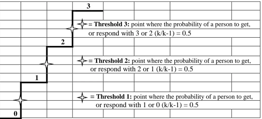
STRONGLY DISAGREE, 1 = DISAGREE, 2 = AGREE, and 3 = STRONGLY AGREE) need to be parametrically separated. In other words, the difficulty of choosing a particular category, say AGREE (let us label it ‘k’) on the scale rather than its lower adjacent category (DISAGREE, k – 1) has an impact on the obtained results, and therefore, it needs to be accounted for by the model. Thus, the RSM adds a third parameter, the threshold parameter, to the original two of the dichotomous model seen above. According to Eckes (2011), this threshold parameter is the location where the adjacent categories, k and k – 1, are equally probable to be observed. An item with four responses, for example 0 = STRONGLY DISAGREE, 1 = DISAGREE, 2 = AGREE, and 3 = STRONGLY AGREE), is modeled as having three thresholds, the first between 0 and 1, the second between 1 and 2, and the third between 2 and 3. „Each item threshold (k) has its own difficulty estimate (F), and this estimate is modeled as the threshold at which a person has a 50/50 chance of choosing one category over another‟ (Bond & Fox, 2007, p. 281). In this respect, it would help to think of scale categories as steps in a staircase:

3

= Threshold 3: point wherethe probability of a person to get, or respond with 3 or 2 (k/k-1) = 0.5

2

= Threshold 2: point wherethe probability of a person to get, or respond with 2 or 1 (k/k-1) = 0.5

1

= Threshold 1: point wherethe probability of a person to get, or respond with 1 or 0 (k/k-1) = 0.5

0

Accordingly, the RSM proposes that the probability of succeeding on a particular item is a function of the person‟s ability, the item difficulty, and the „step difficulty’ (original emphasis) (McNamara, 1996, p. 284), i.e. the difficulty of achieving a score in the k

categories of the scale for each item (Barkaoui, 2013).

The log odds form of the RSM is given by

ln

*

+

= θ

β

- τ

,

where Pnik is the probability that a person n responds with category k to item i; Pnik1 is

the probability that person n responds with category k-1 to item i; k is a response category of a rating scale (= a step in the staircase) that has m + 1 categories, i.e. k = 0, 1, 2, 3, …..m; τkis the difficulty of responding with category k relative to k – 1 (Eckes, 2011, p. 12). For more details about the RSM algebra, see Wright and Mok (2004) and Wright and Masters (1982). A final important word is that the RSM assumes that the step difficulty is the same for all items, which requires the same rating scale be used with all test items, a limitation addressed by the second important extension of the dichotomous model, the Partial Credit Model (PCM).

2.2.2 Masters’ Partial Credit Model (PCM)

Masters (1982) proposed a significant development of the original dichotomous by extending the RSM a step further. He pointed out that some distractors in multiple-choice items could be closer to the correct answer than others, and therefore, they merit some credit as their selection indicates the existence of some knowledge compared to the completely wrong ones, whose selection indicates no knowledge at all (Sick, 2009). Similarly, performance assessment, where different performance levels of the same aspect are displayed, needs to be scored with PCM to discriminate between the levels.

As stated above, the limitation of the Andrich rating scale model (RSM), is that all items “have the same number of steps, and the modelled distance between adjacent steps is consistent across items” (Sick, 2009, p. 7). Masters‟ PCM gains its significance from the fact that it transcends this requirement to allow each item to have its unique rating scale and threshold estimates. Masters (1982) writes: “The model developed in this paper for the analysis of partial credit data is an extension of Andrich‟s Rating Scale model to situations in which response alternatives are free to vary in number and structure from item to item”( p. 150). Wright and Mok (2004) assert that the PCM is similar to the RSM “except that now each item has its own threshold parameters”(p.22). This is achieved by:

ln

*

+

= θn - βi– τik, (10)

thresholds for each item. Such instances are frequent in performance assessment. For example, a student‟s essay or project could be scored as follows:

3 marks: work of a superior quality. 2 marks: work predominantly good quality. 1 mark: satisfactory work.

0 mark: work of poor quality (Wright & Mok, 2004, p. 23).

The above marking criteria show clearly that a score of 3 represents more writing proficiency than that represented by a score of 2, which in turn represents higher proficiency than a score of 1.

3.LINACRE‟S MULTI-FACET RASCH MODEL (MFRM)

The third extension, the focus of this chapter, is the Multi-Facet Rasch Model (MFRM) (Linacre, 1989). It extends Masters‟ PCM to assessment situations, where variables (or

facets) other than person ability and item difficulty systematically impact test outcomes, and therefore, need to be identified and measured (Barkaoui, 2013). Language performance assessment, such as writing and speaking, typically involve not only examinees and items (facets), but also other potentially influential facets such as raters, marking criteria, interviewer, scoring time and space contexts, and possibly many more (Eckes, 2011). MFRM enables test developers to estimate the influence of each facet on the test outcomes by estimating rater severity, and then including that severity estimate in computing the probability of any examinee responding to any task for any scale category threshold for any rater (Barkaoui, 2013; Bond & Fox, 2007). The calibrated facets and their estimates are then placed on the same logit scale for easy comparison. In a writing test, for example, where students respond to a prompt/task by writing essays that are rated by raters/teachers using multiple rating criteria, there are five distinguishable facets of potential influence on the test results: examinee, rater, prompt, marking criteria/rating scales, and the writing feature/aspect each rating scale evaluates. Assuming a constant structure of the rating scale across the elements of the different facets, the multi-facet Rasch measurement model is formally expressed as follows:

ln[

] = θn - βi– Cj - τk, (11)

where,

Pnijk = probability of examinee n receiving a rating of k from rater j on task or aspect (item) i,

Pnijk -1 = probability of examinee n receiving a rating of k - 1 from rater j

on task or aspect (item) i,

θn = proficiency of examinee n, βi = difficulty of aspect (item) i, Cj = severity of rater j,

τk = difficulty of receiving a rating of k relative to k – 1

assessment with a focus on rater-mediated assessment. Before that, a word about the computer program that executes the model expressed in equation (11) is well in place here.

3.1. MFRM analysis: an example

FACETS (Linacre, 2007, 2011) is the computer program that operationalizes MFRM. This program uses the raw scores awarded by raters to test-takers to estimate test-takers‟ abilities, raters‟ severities, task difficulties, and scale category difficulties (Eckes, 2011), and places the obtained estimates onto the logit scale, thus creating a single frame of reference for the interpretation of the results (Bond & Fox, 2007; McNamara, 1996; Myford & Wolfe, 2003; Myford & Wolfe, 2004). It provides information about the reliability of each of these estimates in the form of standard error (SE). It also provides the validity of the measure in the form of fit statistics for each element in each modeled facet” (Bahrouni, 2013; Bahrouni, 2015; Barkaoui, 2013).

In addition, FACETS provides rating scale and bias analyses. Scale analysis evaluates the quality of the rating scale by examining how its categories and category thresholds (scale steps) function, whether they yield meaningful measures, and if their thresholds represent increasing levels of the abilities and the latent traits under investigation (Bahrouni, 2013, 2015; Barkaoui, 2013). Bias analysis, on the other hand, aims at identifying any sub-patterns in the observed scores arising from an interaction of a particular facet, or a particular element within a facet, with another facet, or another element within a different facet, and at estimating the effects of these interactions on the test results (Bahrouni, 2013, 2015; Barkaoui, 2013; Bond & Fox, 2007; Eckes, 2011; Kondo-Brown, 2002; McNamara, 1996; Myford & Wolfe, 2003; Shaefer, 2008).

Results from MFRM analyses allow researchers and testing stakeholders to answer important questions such as these:

1. What effects do the involved facets in the assessment have on test scores? (Barkaoui, 2011, 2013; Kim, 2009; Lumley & O'Sullivan, 2005)

2. What are the interactions, if any, between facets in the assessment context? (Barkaoui, 2013; Kondo-Brown, 2002; Shaefer, 2008; Weigle, 1999)

examinees‟ abilities, raters‟ severity, and the writing features‟ difficulty. It should be noted that except for examinees, all facets are negatively oriented, indicating that high logit measure values mean more severe/difficult, while lower values indicate less severe (= lenient) and less difficult (= easy). The Examinee facet is positively oriented, i.e. high logit measures indicate students that are more able.

FACETS provides various indices for each facet, and for each element within each facet, which inform in general terms on the quality of the test, and the reliability and validity of the results. The most informative of these are the Standard Error (SE), Infit and Outfit Mean Square (IMS and OMS), Strata, Separation Reliability, and Fixed Chi-Square (X2) (Bahrouni, 2013, 2015; Barkaoui, 2011, 2013; Bond & Fox, 2007; G. Jr. Engelhard, 1992, 1994; McNamara, 1996; Myford & Wolfe, 2003; Myford & Wolfe, 2004; Weigle, 1998, 1999).

As stated above, FACETS calibrates the investigated facets in logits units to estimate their effects on the test outcomes, and places obtained estimates on a common logit scale creating a single frame for handy and easy comparison. This single frame displays visually the relationships between facets in the form of a table with a column for each facet, where facet elements are plugged in against the logit scale (the first column on the left) according to their logit measure. In the literature, this particularly useful table is referred to differently as FACETS Variable Map, Wright Map, and Vertical Ruler. (Bahrouni, 2013, 2015; Barkaoui, 2013; Eckes, 2011; McNamara, 1996; Myford & Wolfe, 2003; Weigle, 1998) In the context of this chapter, it is referred to as the Vertical Rulers.

Table 2 Vertical ruler

--- |Measr|+Examinee |-Rater |-Criteria|Scale| ---

+ 1 + + + +(24) +

| | | | | 20 |

| | | | | --- | | | | | | 19 |

| | 2 | | | |

| | | 7 37 | | --- | | | 7 10 11 14 15 | | | 18 |

| | 5 9 | 23 | | |

| | 4 12 | 3 5 9 10 25 31 32 | 4 | --- |

| | 1 13 18 | 8 11 12 14 17 19 21 27 33 38 | 3 | 17 |

* 0 * 6 8 16 17 19 * 4 6 13 20 26 * * * | | | 18 22 30 | 1 2 | --- | | | 3 20 | 2 | | 16 |

| | | 29 34 39 40 | | --- | | | | 1 16 24 35 36 | | 15 |

| | | | | --- | | | | | | 14 |

| | | | | 13 |

| | | | | 11 |

| | | | | 10 |

+ -1 + + + + (0) + --- |Measr|+Examinee |-Rater |-Criteria|Scale| ---

S.1: Model = ?,?B,?B,R25

The Vertical Rulers, hereafter, summarise all the investigated facets, each presented in a separate column with the facet name at the top. Each facet name is preceded by a

facet (examinee) is positively oriented. This means that the more able students have positive measure values, and are therefore placed higher up in the column, while less able ones have negative logit values, and are thus placed lower in the column, bearing in mind, that the average is set to 0.

Take examinees 2 and 3, for example: candidate 2 appears the highest in the column with an ability measure of .52 logits; he/she is the most able among this sample. Examinee 3, on the other hand, appears the lowest in the column because he/she is the least able in this sample with an ability measure of -.29. The second and third facets, however, are negatively oriented. This means that the high-placed elements with positive logit measures are the more severe raters and more difficult criteria, while the low-placed ones with negative values are the more lenient raters and easier criteria. We can see, for instance, that raters 7 and 37 are the most severe in this group of raters, while raters 1, 16, 24, 35, and 36 are the most lenient, and that Grammar (criterion 4) is the most difficult writing feature for students to receive a high score on, while Coherence and Cohesion (criterion 2) is the easiest.

From left to right, the first column is the logit scale against which all elements within each facet are mapped according to their measures (Bahrouni, 2013; Bahrouni, 2015). The second column shows the first facet, examinees, and then comes the second facet, raters, in the third column. The criteria and their scales (third facet) follow in the remaining columns, 4 through 8. Details about each of these facets are provided by

FACETS in subsequent tables generated by the analysis.

The first of these tables shows the Examinee Measurement Report:

Table 3 Examinee measurement report (arranged by Mn)

---

| Obsvd Obsvd Obsvd Fair-M| Model | Infit Outfit |Estim.| | | Score Count Average Avrage|Measure S.E. | MnSq ZStd MnSq ZStd|Discrm| Nu Examinee | | 1 2 3 4 | 5 6 | 7 8 9 10| 11 | 12 | --- | 2850 152 18.8 18.74| .52 .04 | 1.00 .0 .99 .0| 1.07 | 2 E2 | | 2774 152 18.3 18.24| .37 .04 | 1.62 4.4 1.62 4.3| .51 | 7 E7 | | 2768 152 18.2 18.19| .36 .04 | 1.04 .3 1.04 .3| .98 | 14 E14 | | 2760 152 18.2 18.14| .34 .04 | .65 -3.2 .64 -3.3| 1.32 | 15 E15 | | 2747 152 18.1 18.05| .32 .04 | .74 -2.2 .75 -2.2| 1.15 | 10 E10 | | 2745 152 18.1 18.04| .31 .04 | 1.04 .3 1.04 .3| .93 | 11 E11 | | 2709 152 17.8 17.80| .24 .04 | .82 -1.5 .83 -1.4| 1.11 | 9 E9 | | 2674 152 17.6 17.58| .18 .04 | .83 -1.3 .83 -1.3| 1.23 | 5 E5 | | 2651 152 17.4 17.44| .14 .04 | 1.08 .6 1.09 .7| .94 | 4 E4 | | 2636 152 17.3 17.33| .11 .04 | 1.31 2.1 1.24 1.7| .80 | 12 E12 | | 2604 152 17.1 17.18| .06 .04 | 1.05 .4 1.05 .4| 1.01 | 18 E18 | | 2598 152 17.1 17.09| .03 .04 | 1.05 .4 1.06 .4| .95 | 1 E1 | | 2593 152 17.1 17.06| .03 .04 | .84 -1.1 .87 -1.0| 1.07 | 13 E13 | | 2556 152 16.8 16.82| -.04 .04 | .76 -1.9 .76 -1.9| 1.16 | 16 E16 | | 2541 152 16.7 16.73| -.07 .04 | .88 -.8 .86 -1.0| 1.06 | 17 E17 | | 2537 152 16.7 16.70| -.07 .04 | .71 -2.3 .73 -2.1| 1.22 | 8 E8 | | 2519 152 16.6 16.58| -.11 .04 | .66 -2.9 .67 -2.7| 1.27 | 19 E19 | | 2513 152 16.5 16.55| -.11 .04 | 1.71 4.4 1.84 5.1| .35 | 6 E6 | | 2430 152 16.0 16.07| -.23 .04 | .92 -.6 .89 -.8| 1.12 | 20 E20 | | 2392 152 15.7 15.79| -.29 .04 | 1.28 2.0 1.37 2.6| .73 | 3 E3 | --- | Obsvd Obsvd Obsvd Fair-M| Model | Infit Outfit |Estim.| | | Score Count Average Avrage|Measure S.E. | MnSq ZStd MnSq ZStd|Discrm| Nu Examinee | --- | 2629.9 152.0 17.3 17.31| .10 .04 | 1.00 -.1 1.01 -.1| | Mean (Count: 20)| | 120.1 .0 .8 .77| .22 .00 | .29 2.1 .30 2.2| | S.D. (Populn) | | 123.2 .0 .8 .79| .22 .00 | .29 2.2 .31 2.3| | S.D. (Sample) | --- Model, Populn: RMSE .04 Adj (True) S.D. .21 Separation 4.98 Reliability .96

Model, Sample: RMSE .04 Adj (True) S.D. .22 Separation 5.11 Reliability .96 Model, Fixed (all same) chi-square: 537.8 d.f.: 19 significance (probability): .00

Model, Random (normal) chi-square: 18.3 d.f.: 18 significance (probability) : .43

The first four columns comprise simple counts:

Observed score = the total number of points an examinee received from the 38 raters on the four criteria.

Observed count = the number of times an examinee was rated: 38 x 4 = 152.

Observed Average = average from all the raw scores an examinee has received: total number of points received divided by the number of ratings, 2850 points / 152 ratings = 18.75

rounded up to 18.8 (Ex. 2).

Fair Average = the objective score estimated by the model for an examinee. We can easily calculate the total number of points the model estimates examinee 2 to receive by multiplying the fair average by the number of ratings: 18.74 x 152 = 2848.48.

The remaining columns of interest to look at are columns 5, 6 and 7. Column 5 displays the logit measure for each of the calibrated abilities, which range between .52 and -.29 logits, spanning .81 logits. Because this facet is positively oriented, examinees with higher abilities are at the top of the column with positive values, while less able ones are below the average point (0 logit) with negative values. The accuracy of these measures is expressed in column 6 by the Standard Error (SE), which indicates the margin of error for each of these measures. The smaller the SE value (the closer to 0) is, the better. The last column to look at is the Infit Mean Square (IMS), which looks into the extent to which the observed scores fit the model predictions. Briefly, the fit measure informs on the raters‟ consistency in their scoring. The fit limits are set to .6 as the low limit and 1.6 as the high one (Linacre, 1994; Myford & Wolfe, 2003). Values beyond these limits are outliers: any value below .6 indicates overfit (= over predicted = too close to the model prediction, whereas a value over 1.6 is a misfit (= too far from the model prediction). In such cases, a researcher needs to revisit the data to investigate the possible reasons. In case no clear explanation is found, the oft given suggestion in the literature is to discard those elements and re-run the analysis (Bond & Fox, 2007; Engelhard, 1992, 1994; Linacre, 1994; McNamara, 1996; Myford & Wolfe, 2003; Weigle, 1994). The reader may have noticed that there is only one slight misfit case reported in this sample, examinee 7 with an IMS of 1.62.

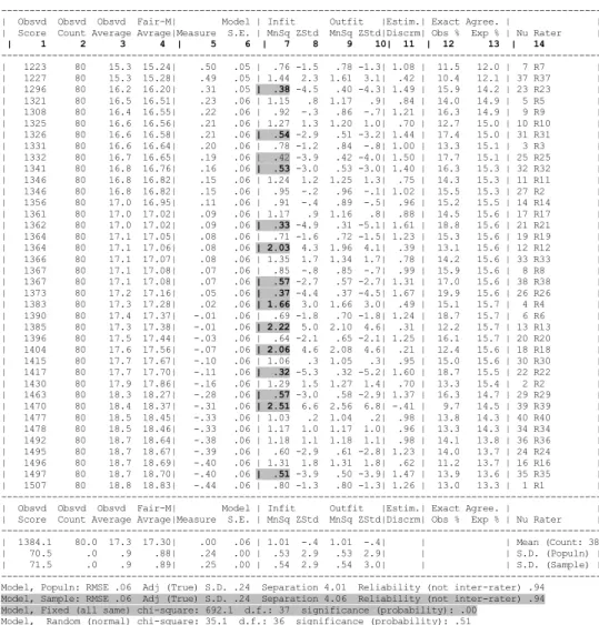
Table 4 Rater measurement report (arranged by Mn)

--- | Obsvd Obsvd Obsvd Fair-M| Model | Infit Outfit |Estim.| Exact Agree. | | | Score Count Average Avrage|Measure S.E. | MnSq ZStd MnSq ZStd|Discrm| Obs % Exp % | Nu Rater |

| 1 2 3 4 | 5 6 | 7 8 9 10| 11 | 12 13 | 14

--- | 1223 80 15.3 15.24| .50 .05 | .76 -1.5 .78 -1.3| 1.08 | 11.5 12.0 | 7 R7 | | 1227 80 15.3 15.28| .49 .05 | 1.44 2.3 1.61 3.1| .42 | 10.4 12.1 | 37 R37 | | 1296 80 16.2 16.20| .31 .05 | .38 -4.5 .40 -4.3| 1.49 | 15.9 14.2 | 23 R23 | | 1321 80 16.5 16.51| .23 .06 | 1.15 .8 1.17 .9| .84 | 14.0 14.9 | 5 R5 | | 1308 80 16.4 16.55| .22 .06 | .92 -.3 .86 -.7| 1.21 | 16.3 14.9 | 9 R9 | | 1325 80 16.6 16.56| .21 .06 | 1.27 1.3 1.20 1.0| .70 | 12.7 15.0 | 10 R10 | | 1326 80 16.6 16.58| .21 .06 | .54 -2.9 .51 -3.2| 1.44 | 17.4 15.0 | 31 R31 | | 1331 80 16.6 16.64| .20 .06 | .78 -1.2 .84 -.8| 1.00 | 13.3 15.1 | 3 R3 | | 1332 80 16.7 16.65| .19 .06 | .42 -3.9 .42 -4.0| 1.50 | 17.7 15.1 | 25 R25 | | 1341 80 16.8 16.76| .16 .06 | .53 -3.0 .53 -3.0| 1.40 | 16.3 15.3 | 32 R32 | | 1346 80 16.8 16.82| .15 .06 | 1.24 1.2 1.25 1.3| .75 | 14.3 15.3 | 11 R11 | | 1346 80 16.8 16.82| .15 .06 | .95 -.2 .96 -.1| 1.02 | 15.5 15.3 | 27 R2 | | 1356 80 17.0 16.95| .11 .06 | .91 -.4 .89 -.5| .96 | 15.2 15.5 | 14 R14 | | 1361 80 17.0 17.02| .09 .06 | 1.17 .9 1.16 .8| .88 | 14.5 15.6 | 17 R17 | | 1362 80 17.0 17.02| .09 .06 | .33 -4.9 .31 -5.1| 1.61 | 18.8 15.6 | 21 R21 | | 1364 80 17.1 17.05| .08 .06 | .71 -1.6 .72 -1.5| 1.23 | 15.3 15.6 | 19 R19 | | 1364 80 17.1 17.06| .08 .06 | 2.03 4.3 1.96 4.1| .39 | 13.1 15.6 | 12 R12 | | 1366 80 17.1 17.07| .08 .06 | 1.35 1.7 1.34 1.7| .78 | 14.2 15.6 | 33 R33 | | 1367 80 17.1 17.08| .07 .06 | .85 -.8 .85 -.7| .99 | 15.9 15.6 | 8 R8 | | 1367 80 17.1 17.08| .07 .06 | .57 -2.7 .57 -2.7| 1.31 | 17.0 15.6 | 38 R38 | | 1373 80 17.2 17.16| .05 .06 | .37 -4.4 .37 -4.5| 1.67 | 19.9 15.6 | 26 R26 | | 1383 80 17.3 17.28| .02 .06 | 1.66 3.0 1.66 3.0| .49 | 15.1 15.7 | 4 R4 | | 1390 80 17.4 17.37| -.01 .06 | .69 -1.8 .70 -1.8| 1.24 | 18.7 15.7 | 6 R6 | | 1385 80 17.3 17.38| -.01 .06 | 2.22 5.0 2.10 4.6| .31 | 12.2 15.7 | 13 R13 | | 1396 80 17.5 17.44| -.03 .06 | .64 -2.1 .65 -2.1| 1.25 | 16.1 15.7 | 20 R20 | | 1404 80 17.6 17.56| -.07 .06 | 2.06 4.6 2.08 4.6| .21 | 12.4 15.6 | 18 R18 | | 1415 80 17.7 17.67| -.10 .06 | 1.06 .3 1.05 .3| .95 | 15.0 15.6 | 30 R30 | | 1417 80 17.7 17.70| -.11 .06 | .32 -5.3 .32 -5.2| 1.60 | 18.7 15.5 | 22 R22 | | 1430 80 17.9 17.86| -.16 .06 | 1.29 1.5 1.27 1.4| .70 | 13.3 15.4 | 2 R2 | | 1463 80 18.3 18.27| -.28 .06 | .57 -3.0 .58 -2.9| 1.37 | 16.3 14.7 | 29 R29 | | 1470 80 18.4 18.37| -.31 .06 | 2.51 6.6 2.56 6.8| -.41 | 9.7 14.5 | 39 R39 | | 1477 80 18.5 18.45| -.33 .06 | 1.03 .2 1.04 .2| .98 | 13.8 14.3 | 40 R40 | | 1478 80 18.5 18.46| -.33 .06 | 1.17 1.0 1.17 1.0| .96 | 13.3 14.3 | 34 R34 | | 1492 80 18.7 18.64| -.38 .06 | 1.18 1.1 1.18 1.1| .98 | 14.1 13.8 | 36 R36 | | 1495 80 18.7 18.67| -.39 .06 | .60 -2.9 .61 -2.8| 1.23 | 14.0 13.7 | 24 R24 | | 1496 80 18.7 18.69| -.40 .06 | 1.31 1.8 1.31 1.8| .62 | 11.2 13.7 | 16 R16 | | 1497 80 18.7 18.70| -.40 .06 | .51 -3.9 .50 -3.9| 1.47 | 13.9 13.6 | 35 R35 | | 1507 80 18.8 18.83| -.44 .06 | .80 -1.3 .80 -1.3| 1.26 | 13.0 13.3 | 1 R1 | --- | Obsvd Obsvd Obsvd Fair-M| Model | Infit Outfit |Estim.| Exact Agree. | | | Score Count Average Avrage|Measure S.E. | MnSq ZStd MnSq ZStd|Discrm| Obs % Exp % | Nu Rater | --- | 1384.1 80.0 17.3 17.30| .00 .06 | 1.01 -.4 1.01 -.4| | | Mean (Count: 38| | 70.5 .0 .9 .88| .24 .00 | .53 2.9 .53 2.9| | | S.D. (Populn) | | 71.5 .0 .9 .89| .25 .00 | .54 2.9 .54 3.0| | | S.D. (Sample) | --- Model, Populn: RMSE .06 Adj (True) S.D. .24 Separation 4.01 Reliability (not inter-rater) .94

Model, Sample: RMSE .06 Adj (True) S.D. .24 Separation 4.06 Reliability (not inter-rater) .94 Model, Fixed (all same) chi-square: 692.1 d.f.: 37 significance (probability): .00

Model, Random (normal) chi-square: 35.1 d.f.: 36 significance (probability): .51

Inter-Rater agreement opportunities: 56240 Exact agreements: 8284 = 14.7% Expected: 8361.5 = 14.9% ---

The depicted differences between the raters‟ severity levels are quite reliable (.94) and significant. Having a group of homogeneous raters, who interpret and apply the rating scale in a similar way, is obviously the utmost goal of all test stakeholders. However, before concluding about its genuineness, a researcher ought not be over optimistic about this homogeneity, and ought to explore other potential influential factors, such as rater central tendency, functioning of the rating scale, the unexpected responses (residuals), and the fit statistics, which are a source of concern in this context, because we can already see that 15 raters have been found inconsistent in their ratings: ten (10) overfit and five (5) misfit cases have been reported.

Coming to the last facet in this demonstration, the four criteria/writing features are ordered according to their difficulty. This facet is also negatively oriented. As explained above, this means that the difficult criteria have positive values, while the easy ones have negative values. According to the separation index, their difficulty level, which spans .29 logits with grammar as the most difficult (.16) and coherence as the easiest (-.13), is split into seven distinguishable, highly reliable (.98) and significant (.00) levels of difficulty. The four criteria have all been reported to fit the model.

Table 5 Criteria measurement report (arranged by Mn)

--- | Obsvd Obsvd Obsvd Fair-M| Model | Infit Outfit |Estim.| | | Score Count Average Avrage|Measure S.E. | MnSq ZStd MnSq ZStd|Discrm| N Criteria | --- | 12683 760 16.7 16.81| .16 .02 | .97 -.5 1.02 .2| 1.00 | 4 GR | | 12996 760 17.1 17.17| .06 .02 | .90 -1.6 .91 -1.6| 1.12 | 3 VOC | | 13388 760 17.6 17.64| -.09 .02 | 1.20 3.1 1.19 3.0| .85 | 1 TA | | 13530 760 17.8 17.80| -.13 .02 | .97 -.5 .97 -.5| 1.04 | 2 CC | --- | 13149.3 760.0 17.3 17.35| .00 .02 | 1.01 .1 1.02 .3| | Mean (Count: 4) | | 332.7 .0 .4 .39| .12 .00 | .11 1.8 .10 1.7| | S.D. (Populn) | | 384.2 .0 .5 .45| .14 .00 | .13 2.1 .12 2.0| | S.D. (Sample) | --- Model, Populn: RMSE .02 Adj (True) S.D. .12 Separation 6.20 Reliability .97

Model, Sample: RMSE .02 Adj (True) S.D. .13 Separation 7.18 Reliability .98 Model, Fixed (all same) chi-square: 160.7 d.f.: 3 significance (probability): .00 Model, Random (normal) chi-square: 2.9 d.f.: 2 significance (probability): .23

---Turning to bias analysis, it investigates whether one particular aspect of the test shows a consistently biased pattern of scores (Barkaoui, 2013). McNamara (1996) explains that bias analysis in MFRM consists essentially of comparing residuals, i.e. the differences between the expected and the observed values. Once the overall rater severity, the examinee‟s ability, and the criteria difficulty have been estimated across the board, MFRM estimates the most likely score for each examinee by a given rater on a particular criterion assuming consistency of that particular rater‟s way of scoring across all criteria (Barkaoui, 2013; McNamara, 1996). These individual scores are totalled across all examinees to yield a total expected score from each rater on each criteria, which is then compared to the observed total score for all examinees (Barkaoui, 2013). Thus, if the observed total score criterion is lower than the expected score, then this criterion appears to have elicited more severity than usual on the part of the raters, and vice versa. This difference is expressed in a logit measure, which tells the investigator how much of a challenge this criterion presented when scored by this particular rater, and the effect of this challenge on the chances of success for examinees in such contexts (Barkaoui, 2013; McNamara, 1996).

scales in the same way (= inter-rater inconsistency), b) raters were not self-consistent (= intra-rater inconsistency), and c) the rating scales were not functioning properly. A researcher faced with such a situation out to seek explanation in these three areas.

4.CONCLUSION

To spell out the important usefulness of MRFM for eliciting objective measures in rater-mediated assessment contexts, this paper has shown the theoretical framework that laid the groundwork for the emergence of the Rasch Measurement Theory. Then it has walked the reader through the conceptual chronological developments that brought about MFRM. For demonstration, a live data sample has been used to show the MFRM operationalization through the computer program, FACETS. The main features and indices of FACETS analysis have been explained in the demonstration. The Data and Run files are included hereafter, as appendices, for readers who want to try it. A free downloadable mini version of FACETS is available at www.winsteps.com/minifac.htm. The interested reader may also benefit from unstinting support provided by the Rasch Forum at http://raschforum.boards.net/.

To learn more about FACETS technical features and how to run the program, see Myford (2008) and Bond and Fox (2007, pp. 277-298)

MFRM has proved to be a valuable tool to investigate the effects of various facets on test outcomes in rater-mediated assessment contexts. However, a researcher has to be well aware of the concerns discussed above when using and interpreting results from MFRM analysis.

APPENDICES

To see the appendices, click on the link below:

https://docs.google.com/document/d/1cX1TLbM76U5MfDlbFasBQVeEf4J_uWKuYTm quthFS5I/edit?usp=sharing

ACKNOWLEDGEMENT

The author wants to express his sincere gratitude to Sultan Qaboos University and its Language Centre for supporting the study that provided the dataset used in this paper to illustrate FACETS analysis.

REFERENCES

Bahrouni, F. (2013). Impact of empirical rating scales on EFL writing assessment. In S. Al-Busaidi & V. Tuzlukova (Eds.), Genaral Foundation Programmes in Higher Education in the Sultanate of Oman: Experiences, Challenges and Considerations for the Future (pp. 256 - 302). Muscat: Mazoon Press and Publishing.

Barkaoui, K. (2011). Effects of marking method and rater experience on ESL essay scores and rater performance. Assessment in Education: Principles, Policy & Practice, 18(3), 279-293.

Barkaoui, K. (2013). Multi-faceted Rasch Analysis for Test Evaluation. Companion to Language Assessment. III:10:77, 1301–1322. doi: 10.1002/9781118411360.wbcla070 Bond, T. G., & Fox, C. M. (2007). Applying the Rasch Model: Fundamental

Measurement in the Human Sciences. (2nd ed.): Laurence Erlbaum.

Eckes, T. (2011). Introduction to Many-Facet Rasch Measurement: Analyzing and Evaluating Rater-Mediated Assessments (Vol. 22): Peter Lang.

Engelhard, G. J. (1992). The Measurement of Writing Ability With a Many-Faceted Rasch Model. Applied Measurement in Education, 5(3), 171-191.

Engelhard, G. J. (1994). Examining Rater Errors in the Assessment of Written Composition With a Many-Faceted Rasch Model. Journal of Educational Measurement, 31(2), 93-112. Engelhard, G. J. (2013). Invariant Measurement: Using Rasch Models in the Social,

Bahavioral, and Health Sciences: Routledge.

Farrokhi, F., & Esfandiari, R. (2011). A Many-facet Rasch Model to Detect Halo Effect in Three Types of Raters. Theory and Practice in Language Studies, 1(11), 1531-1540. Furr, R. M., & Bacharach, V. R. (2007). Item Response Theory and Rasch Models

Psychometrics: An Introduction (1 ed.): SAGE Publications.

Kim, Y. (2009). An investigation into native and non-native teachers' judgments of oral English performance: A mixed methods approach. Language Testing, 26(2), 187-217. Kondo-Brown, K. (2002). A FACETS analysis of rater bias in measuring Japanesse

second languagewriting performance. Language Testing, 19(1), 3-31.

Linacre, J. M. (1994). Many-Facet Rasch Measurement. Chicago: MESA PRESS. Lumley, T., & O'Sullivan, B. (2005). The effect of test-taker gender audience & topic on

task performance in tape-mediated assessment of speaking. Language Testing, 22(4), 415-437.

Masters, G. N. (1982). A Rasch Model for Partial Credit Scoring. Psychometrika, 47(2), 149-174.

McNamara, T. F. (1996). Measuring Second Language Performance. London: Longman. Myford, C. M. (2008). Analyzing Rating Data Using Linacre's Facets Computer Program: A set of Training Materials to Learn to Run the Program and Interpret Output. University of Chicago.

Myford, C. M., & Wolfe, E. W. (2003). Detecting and Measuring Rater Effects Using Many-Facet Rasch Measurement: Part I. Journal of Applied Measurement 4(4), 386-422. Myford, C. M., & Wolfe, E. W. (2004). Detecting and measuring rater effects using

many-facet Rasch measurement: Part II. Journal of Applied measurement, 5(2), 189-227. Shaefer, E. (2008). Rater bias patterns in an EFL writing assessment. Language Testing,

25(4), 465-493.

Sick, J. (2008). Rasch Measurement in Language Education: Part 1. Shiken: JALT Testing & Evaluation SIG Newsletter, 12(1), 1-6.

Sick, J. (2009). Rasch Measurement in Language Education Part 3: The family of Rasch Models. Shiken: JALT Testing &Evaluation SIG Newsletter, 13(1), 4-10.

Weigle, S. C. (1998). Using Facets to model rater-training effects. Language Testing, 15(2), 263-287.

Weigle, S. C. (1999). Investigating Rater/Prompt Interations in Writing Assessment: Quantitative & Qualitative Approaches. Assessing Writing, 6(2), 145-178.

Wind, A. S. (2014). Evaluating Rater-Mediated Assessments with Rasch Measurement and Mokken Scaling. Emory.

Wright, B. D., & Masters, G. N. (1982). Rating Scale Analysis: Rasch Measurement. Chicago: MESA Press.