5521.pdf

(1)

BAYESIAN NONPARAMETRIC

DIFFERENTIAL EQUATION MODELS FOR

FUNCTIONS

Matthew W. Wheeler

A dissertation submitted to the faculty of the University of North Carolina at Chapel Hill in partial fulfillment of the requirements for the degree of Doctor of Philosophy in the Department of Biostatistics.

Chapel Hill 2013

Approved by:

Dr. Amy H. Herring Dr. David B. Dunson Dr. Eric Bair

(2)

c

2013

(3)

Abstract

MATTHEW W. WHEELER: Bayesian Nonparametric Differential Equation Models for Functions

(Under the direction of Dr. Amy H. Herring and Dr. David B. Dunson)

Bayesian nonparametric methods develop priors over a large class of functions that essentially allow any continuous function to be modeled. Though these methods are flexible, they are black box approaches that do not explicitly incorporate additional information on the shape of the curve. In many contexts, though the exact parametric form of the curve is unknown, additional scientific information is available in the form of differential operators. This dissertation develops nonparametric priors over func-tion spaces that are specified by differential operators. Here two novel approaches to nonparametric function estimation are considered. In the first approach the prior is specified by a linear differential equation. The Mechanistic Hierarchical Gaussian pro-cess defines a prior over functions consistent with a differential operator. The method is applied to muscle force tracings in a functional ANOVA context, and is shown to adequately describe the between subject variability often seen in such tracings. In the second case a novel spline based approach is considered. Here prior information is spec-ifies the maximum number of extrema (changepoints) for an arbitrary function located on an open set in _R. The Local Extrema (LX) spline models the first derivative of the curve and puts a prior over the maximum number of changepoints. This method is applied to animal toxicology studies, human health surveys, and seasonal data; and it is shown to remove artifactual bumps common to other nonparametric methods. It is further shown to superior in terms of estimated squared error loss in simulation

(4)

(5)

To my wife Kimberly and all of those sleepless nights you wanted to kill me. To my parents who taught me right from wrong.

Finally to Hank: “And then came the revolution.”

(6)

Acknowledgments

I would first and foremost thank my wife Kimberly. If it were not for your prayers, love, support, and your insistence on staying in North Carolina this dissertation would have never been written. You are the love of my life, and I thank God everyday for you.

I would also like to thank my advisors David and Amy. Your guidance and insights were invaluable. David, quite honestly, if it was not for you being such a hard ass, I would have never improved. My writing might still suck, but it sucks much much less. Thanks for putting up with me for the past three years.

A special thank you goes to John Bailer. If it were not for an hour long conversation between Upham and Gaskill in the Fall of ‘06 I would have never applied to UNC, and this would have never happened.

I would also like single out Dustin and Leann Long. Dustin for putting up with a papist – I still say the reformation was a dumb idea – and Leann for studying with me all those hours leading up to our qualifiers as well as lending me your husband to talk about obscure topics no one gives a shit about. You both are pretty damn good people – for Methodists.

(7)

Also I would like to take a moment and apologize to all I pissed off/put off with my gruff exterior. For me, this dissertation was more about expelling past demons than professional advancement, and exorcisms are always difficult business. They are even more difficult when you are surrounded by people, who through no fault of their own, remind you of all of the people who told you you were stupid, ignorant, and backwards most of your life. It was never my fault (nor my families) that I came from a non-college educated working class family whom by many of the PC intelligentsia would be considered uneducated bigots in ’polite conversation’. Further, I should not be at fault if I saw no reason to prefer the new culture I have lived in reluctantly for the past 5 years over the one I grew up in. However, it was not your fault that you might have been caught up in the war that has raged in my head the past 5 years, and for that I apologize.

Finally a must acknowledge my three children Megan, Jeni, and Claire. I did this for you. If you don’t fight for what you believe in and pick yourself up when you fall who will? This document is a testimony to that fact and you should not forget this. Finally, Claire, though you are much too young to read this, I thank you for that 3 a.m. feeding where I first thought about the LX-spline. Your giggles made finishing this document a little more bearable. -AMF

(8)

List of Tables

4.1 Ratio of squared error loss between the LX-spline and the P-spline for line segments on X = [2,3] given a specified derivative and variance condition. . . 96

4.2 Results of a simulation study looking at the posterior probability (with corresponding 95% confidence intervals) the estimated curve contains a single minimum when compared to a monotone increasing curve for three simulation conditions. The three conditions considered for the true curve were: monotone increasing (i.e., no minimum), shallow minimum near the boundary of X, and a well defined minimum. . . 97

4.3 Summary of hepatocellular adenomas data of female B6CF1 mice ex-posed to tumeric oleoresin. The top three lines show control data for NTP studies that were used to develop priors for the analysis. . . 98

(12)

List of Figures

2.1 The first and second lines represent the beginning of the isometric and stretch shortening contraction, respectively. The third and fourth lines represent the end of the stretch shortening and isometric contractions, respectively. . . 40

2.2 Estimated group level curves for the dynamic force in a stretch shortening contraction. Solid line, and corresponding 95% credible region (dotted line), representing the estimated curve. Here truth is represented by the dashed line. . . 41

2.3 The estimated mean isometric force generated for a single animal pre and post treatment. The dark black line represents central estimates of Q(t)F(t), with the dark gray hash marks representing the observed data. Here credible interval estimates are not shown as they are very narrow. 42

2.4 The estimated group level dynamic force multiplier generated by young (right column) and old (left column) animals. The bottom row represents the 95% pointwise credible interval for this difference. . . 43

2.5 Estimated mean isometric muscle force generated for the young animals pre (dashed line) and post (solid line). The bottom row gives the es-timates, and 95% pointwise credible intervals of the difference between the two. . . 44

2.6 Estimated dynamic muscle force for an old animal. Here the top figure is the central estimate for the pre (dash dotted line) and post (solid line), and the bottom figure is the estimated difference between the two estimates. . . 45

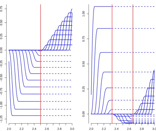
3.1 LX splines with a single changepoint at 2.5 (left), and LX splines with two changepoints at 2.33 and 2.66 (right). . . 61

3.2 Estimated squared error loss between the GP and the LX-spline from simulation condition 1, for the first condition of all three shapes investi-gated. . . 62

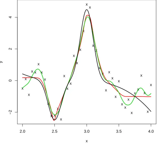
3.3 Estimation of f3(x) (black) using the LX-spline (red) and the smoothing

(13)

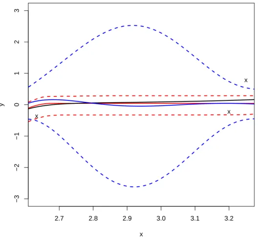
3.4 Estimated curve (solid red line) and 95% confidence intervals (dashed red line) for the LX-splines, and the Gaussian process ( blue solid and dashed lines respectively) when estimating the true curve (black). . . . 64

3.5 Fit of the Albany, NY temperature data when using smoothing splines (red) and P-splines (blue). . . 65

3.6 Fit of the LX spline (red) as compared to the Gaussian process (blue) based upon 3 years of daily high temperature data collected in Albany, NY. . . 66

3.7 Relative risk of all cause mortality estimated using a spline based approach. 67

3.8 Estimated relative risk of all cause mortality, and corresponding 95% confidence intervals for different BMIs calculated using the LX spline only. Here risk is relative to the BMI associated with the minimum risk (BMI = 30.03). . . 68

4.1 Order restricted splines with a single change point at 2.5 (left), and order restricted splines with two change points at 2.33 and 2.66 (right). . . . 90

4.2 Fit of the LX-spline (black line) with corresponding 95% credible inter-vals (dotted line) and Bayesian P-spline (red) for the top and bottom plots. The top plot represents a simulation with lower variance and the bottom plot represents a higher variance condition. . . 91

4.3 Plot of the observed total fertility rate against the HDI. The gray solid line represents the results reported (Myrskyl¨a et al. 2009). The LX-spline is show using the solid black line, with corresponding 95% credible intervals of the LX-spline fit to the same data. . . 92

4.4 The top plot shows the seasonally adjusted world CO2 trend line (dashed

line) as compared to the seasonally unadjusted estimate (dark black line) fit to the observed data. The bottom plot compares the seasonally adjusted world CO2 estimate where the adjustment was based upon the

LX-spline (dashed line) and the X−12 ARIMA adjustment (solid line). 93 4.5 Estimated seasonal adjustment for the observed yearly CO2

concentra-tion data (black line) and its 95% estimated credible interval (dotted line). . . 94

4.6 Estimated dose-response curve for tumeric oleoresin in a two year bioas-say of B6CF1 female mice. The curve represents the probability of ob-serving hepatocellular adenomas given increasing levels of tumeric oleo-resin (ppm). . . 95

(14)

Chapter 1 Literature Review

Bayesian data analysis proceeds by positing that, given a sequence of data Y = (y1, . . . , yn),one can learn about the underlying generating mechanism through a series

of simplifying assumptions. This is done by assuming data arise from a sampling model P(Y|Θ) controlled by parameter vector Θ. In a Bayesian analysis one assumes that Θ is a random quantity, and that its uncertainty can be quantified a priori by P(Θ), a probability measure over possible values of Θ. The quantity P(Θ) is prior knowledge on Θ, and we wish to update this prior belief given new information. Learning is accomplished through the use of Bayes Rule

P(Θ|Y) = R P(Y|Θ)P(Θ)

P(Y|Θ)P(Θ)dΘ,

which updates the distribution for Θ in the presence of new informationY.

Bayesian analyses often proceed by assuming that the data vector Y comes from a known distribution, and that Θ enters into this distribution with parametric form known a priori. For example linear regression assumes Y = XΘ + where ∼

N(0, σ2_I

n). This implies that Y ∼ N(XΘ, σ2In), which forces explicit structure on

(15)

study. Strong assumptions may not be warranted, and may not fully encapsulate the uncertainties in the system of interest. In the above example multiple assumptions may be called into question. First the normality assumption may be unrealistic as it assumes that the data arise from a unimodal distribution having relatively light tails. Also the linearity assumption may also be called into question as it is overly restrictive of the functional form. Such analyses may lead to unrealistic inference.

An alternative to such restrictive assumptions is to develop priors which are more reflective of the uncertainty in the system of interest. Such approaches put priors over a rich class of both probability measures and function spaces that better reflect the uncertainties in the system. For example, the Dirichlet prior (Ferguson 1973; 1974) and other stick breaking priors (Sethuraman 1994; Ishwaran and James 2001) can be used to define priors over the space of probability measures. As these priors are almost surely discrete, they are frequently used in combination with mixing kernels such as the Dirichlet mixing process (DPM) (Lo 1984), which can then be used to develop priors over the space of distribution functions that do not assume a specific parametric form onP(Y|Θ).

Similarly, priors over functional forms can be developed to circumvent the use of simplifying assumptions such as linearity in the mean response, i.e.,E[Y] =XΘ. Here versatile priors, such as the Gaussian process (GP) (Rasmussen and C. 2006), can be used to define a prior over a large set of smooth functions in_Rp_{. Such an approach, when}

combined with the DPM approach, allows one to define priors having large support over possible generating mechanisms. These approaches may be better in encapsulating the uncertainties in the system under study.

In what follows many aspects of non-parametric Bayesian inference are reviewed. Section (1.1) reviews stick breaking priors such as the Dirichlet process, and section (1.2) reviews non-parametric Bayesian regression methods.

(16)

1.1 The Dirichlet process prior and other stick-breaking priors

Much of the recent work in Bayesian non-parametrics has focused on the use of the Dirichlet process (Ferguson 1973; 1974; Sethuraman 1994), and other stick-breaking pri-ors (Ishwaran and James 2001). Given a complete and separable metric space (Θ,B), a stick-breaking prior G defines a prior over P, the collection of probability measures on (Θ,B). In other words, if one definesC to be the smallest σ−field generated by sets of the form{P :P(θ)< k} where θ∈ B,P ∈ P and k∈[0,1],then the stick-breaking prior G, defines a probability measure over (P,C). Given any finite measurable parti-tion {θ1, θ2, . . . , θL} of Θ, G defines a prior probability measure over sets of the form {P(θ1), P(θ2), . . . , P(θL)}.Such priors allow one to learn about an arbitrary probability

measureP given Y using Bayesian methods.

Stick-breaking priors are unique in that they admit a specific construction on G.A prior Ghas a stick-breaking representation if and only if

G(·) =

L X

h=1

whδθh(·), (1.1)

where δθh(·) is a discrete measure concentrated at θh ∈ Θ, and {wh}h=1 are weights such that 0 ≤ wh ≤ 1 and PL_h wh = 1. Each weight is constructed from a set of

random variables{Vh}Lh=1defined on (0,1) whereVh ∼H,andH is a known probability

measure. The stick breaking construction defines {wh}Lh=1 through

w1 =V1 (1.2)

and

wk =Vk k−1 Y

h=1

(17)

In this construction the first few weights (i.e w1, w2, . . . etc.) receive a large portion

of the prior mass, with each subsequent weight receiving a geometrically diminishing probability. This implies only a few atoms θi ∈ Θ receive a large prior probability of

being selected. Note that the total number of atomsLmay be finite, or countably infi-nite. This construction in (1.1) is completed by noting that{θh}Lh=1 are independently

drawn from a base line measure G0 and are independent from the weights.

In applications theVkare often taken as independentBeta(ak, bk) random variables.

Both the Dirichlet (Ferguson 1973) and Pittman-Yor processes (Pitman 1996; Pitman and Yor 1997) can be shown to be stick-breaking processes as in (1.1). By takingL=∞, ak = 1, and letting bk = b for all k, one arrives at the Dirichlet process (Sethuraman

1994). Also by taking L = ∞, setting ak = 1−a and bk = b +ka), for 0 ≤ a < 1

and b > −a, one constructs the Pittman-Yor PY(a, b) process (Pitman 1995). The Vk are not necessarily limited to beta random variables, and other possibilities have

been explored (e.g., Rodriguez and Dunson (2011)). Rodriguez and Dunson (2011) defined the probit stick-breaking process using standard normal random variables, and constructed weights using Vk = Φ(ak) whereak∼N(0,1).

The stick-breaking construction is almost surely discrete, which limits its usefulness for most applications. Instead of being used as a prior for observed data, it is frequently employed as a prior over weights in mixture modeling. That is, given some parametric densityg, a prior over possible data generating mechanisms is specified as

fG(y) = Z

g(y;θ)dG(θ). (1.4)

Such a mixture distribution was originally proposed by Lo (1984) withGis defined as a Dirichlet process. This approach defines a rich prior over a variety of distributions and can be used in for continuous density estimation as well as repeated measures data.

(18)

Direct estimation of the posterior distribution of such stick-breaking mixture mod-els is unavailable in closed form, and various MCMC methods have been developed to sample from the posterior distribution. These methods generally can be divided into two categories. The first marginalizes over the stick-breaking process relating the process to the Polya urn model. The second approach samples the full conditional distribution. Here the weights and the unique atoms{θ_h∗}L

h=1are sampled conditionally

on the other terms of the model.

Generalized Polya-Urn Sampling

This sampling method is related to the Polya urn model that Blackwell and MacQueen (1973) connected to the Dirichlet process. It was later shown by Pitman (1996) that when Vk ∼ Beta(ak, bk) the stick-breaking process can be characterized in term of a

generalized Polya-Urn mechanism, and can be used when the Vk are drawn from a

Beta(ak, bk) distribution. For clarity the sampling method is first described in relation

to the Dirichlet process and then generalized in relation Pittman-Yor model.

In the Polya-Urn model colored balls are drawn from an urn in succession. After each draw, the drawn ball is put back in the urn along with C balls of the same color. Once a ball is drawn there is an increased probability of it being drawn in the future. Blackwell and MacQueen (1973) noted that by marginalizing over the Dirichlet process one arrives at the Polya urn model. As draws from this model can be shown to be exchangeable, any draw in the process can be taken conditionally with respect to the other draws.

Given a Dirichlet process G ∼ DP(bG0) where b is the weight parameter, and G0

(19)

showed that the conditional distribution drawing θi given the previous draws is

θi|θ1, θ2, . . . , θi−1 ∼

b

b+i−1G0+

i−1 X

k=1

1

b+i−1δθk(·).

Here Individual atoms can be thought of as being drawn from the urn in succession. For each draw there is a uniform probability of the next atom drawn as being any one of the previous draws, and a positive probability proportional to G0 of the next draw

being drawn from the base measure. As there may be ties (i.e., θi = θj for i6= j) one

can equivalently defineθ₁∗, θ₂∗, . . . , θ_L∗ as theLunique atoms that have been drawn from the urn. Letting defining m1, m2, . . . , mL be the number of times each atom has been

drawn, the probabilities specified above can be re-expressed as

θ_i∗|θ₁∗, . . . , θ_i∗₋₁, θ∗_i₊₁, . . . , θ_L∗ ∼ b

b+i−1G0+

i−1 X

k=1

mk

b+i−1δθ∗k(·).

With this representation it one can see that successive draws of the same atom increases the probability the atom is drawn in the future. Observations tend to cluster around distinct atoms often resulting in fewer atoms than observations. This clustering of draws can be seen as a feature of the stick-breaking process where there exists a high probability of the next atom being drawn from one of a small number of atoms.

Such conditional probabilities can be generalized to any PY(a, b, G0) process. The

probability of the current draw, conditional on the previous draws, is

P r(θi =θj∗|θ

∗

1, . . . , θ

∗

L) =           

mj−a

b+i−1 j ≤L b+aL

b+i−1G0 otherwise

(1.5)

The Polya-urn scheme can be used to sample from mixture distribution as in (1.4). This connection was first utilized by Escobar (1994) and Escobar and West (1995) to

(20)

formulate MCMC sampling methods for Dirichlet mixture processes, under the con-jugate assumption that g(·) and G0 are both Gaussian. It can further be applied to

priors on G0.

I focus on an general algorithm that includes both the conjugate and non-conjugate cases. Given observed data vector (y1, y2, . . . , yn)0,we wish to sampleθ = (θ1, θ2, . . . , θn)0,

which are then latent quantities distributedG, which is a vector of quantities defining the relation yi|θi ∼ g(yi;θi). Letting {θ∗k}

L

k=1 to be the set of unique draws from the

urn, andθ−i the vectorθ without entryi, the algorithm proceeds for anyPY(a, b, G0)

as follows:

1. For each i,i= 1, . . . , ndraw θi from

θi|θ−i ∼

b+aL

b+i−1q0G0 +

i−1 X

k=1

mk−a

b+i−1g(yi;θ

∗

k)δθ_k∗(·). (1.6)

whereq0 = R

g(yi;θ)dG0(θ).It is possible thatθiis the only member in the cluster

implying that the set{θ_k∗}L

k=1 should be recomputed for each draw.

2. For each k, k= 1, . . . , L and each yi allocated to cluster k drawθk∗ from

θ_k∗ ∝G0(θ∗k) Y

{yi:θi=θ∗k}

g(yi;θk∗) (1.7)

In cases where G0 is non-conjugate with the kernel g(·;θ) the integral representation

of q0 may be intractable. Various computational methods to ease (MacEachern and

M¨uller 1998; Neal 2000) have been developed.

(21)

i is assigned to θ∗_k.One proceeds by first sampling the augmented cluster membership variable and then updating{θ∗_k}L

k=1 given this membership variable. Conditional Methods

As mixing for the Polya-urn sampler is often poor and non-conjugate sampling can be difficult, various methods have been developed to sample from the posterior conditional on knowledge of the weights. These methods, which are often termed conditional methods, frequently provide better mixing than methods based upon the Poly-urn scheme. The first of such methods described are the block Gibbs sampling methods of Ishwaran and Zarepour (2000) and Ishwaran and James (2001).

These methods approximate the infinite stick breaking process G through a finite dimensional truncation of the posterior distribution. Given the proper truncation level, these methods define a prior that can be shown to be arbitrarily close to the desired countably infinite stick breaking process. Let L be the number of elements in the truncation. To create an truncation of an infinite stick breaking process one discards the wL+1, wL+2,· · · weights by setting wL = 1−w1−w2− · · ·wL−1. This construction

can be shown to have a marginal density µL(Y) that is arbitrarily close to µ∞(Y) for

large L. Define k · k to be the L1 distance, then (Ishwaran and James 2001) showed

that

kµL(Y)−µ∞(Y)k ≤4 1−E

" _L₋₁

X

k=1

pk

!n#!

. (1.8)

This implies that if the stick breaking weights are constructed such thatEhPL−1 k=1 wk

ni

→

1 as L → ∞there should be little difference between the finite truncation model and the countably infinite stick breaking process. It can be shown for both the Dirichlet and Pittman-Yor processes that accurate truncations exist. For the PY(a, b) process

(22)

one has

kµL(Y)−µ∞(Y)k ≤4(1−E[1−( ∞

X

k=L

wk)n]) (1.9)

and for the Dirichlet process this expression simplifies to

kµL(Y)−µ∞(Y)k ∼4 n exp(−(L−1)/b). (1.10)

As a consequence on can create a finite truncation that is virtually indistinguishable from the infinite stick-breaking prior whenL is moderately large.

As sampling fromGL is computationally simpler than sampling fromG, block

sam-pling can accurately approximate the infinite stick breaking process. We describe the algorithm in terms of Vk ∼Beta(ak, bk), noting that for generalVk ∼ H slight

modifi-cations are needed. The algorithm introduces a latent variableξi for each observation.

Hereξi =k if and only if observation yi is allocated to clusterk.

1. Sample θ∗|Y,ξ: For each K, such that 1≤k ≤Lsample from the density

θ∗_k|Y,ξ∝G0(θk) Y

i:ξi=k

g(yi|θk∗)

2. Sample ξ|θ∗, p: For each i= 1, . . . , n sampleξi from

ξi|θ∗,ξ, Y ∼M ultinomial(p1i,· · · , pLi) (1.11)

wherepki ∝pkg(yi|θki)

(23)

the multinomial distribution we have

Vk∼Beta(ak+Mk, bk+ L X

l=k+1

Ml), (1.12)

where Mk = Pn_i₌₁1(ξi ≥ k). Given V1, . . . , VL−1 one can calculate the p0ks as in

(1.2) and (1.3).

As the value of the finite truncation level is chosen a priori some caution is needed when using a block sampler. Values of L that are too small may lead to inference from a posterior that does not closely approximate the infinite stick-breaking process. Conversely values of L that are too large unnecessarily increase the computational burden.

Other methods have been developed to avoid the truncation problem, which allow sampling from the exact distriutionG. Papaspiliopoulos and Roberts (2008) proposed one such method. This algorithm modifies the above by lettingLchange across MCMC iterations. Again letting Lbe the current number of atoms in the sampler a retrospec-tive sampler introduces an auxiliary variable Ui ∼ U nif orm(0,1) setting ξi = j if

Pj−1

k=1pk < Ui <

Pj−1

k=1pk, with more weights/atoms introduced if

PL

k=1pk < Ui. This

method allows one to sample from a countably infinite stick breaking process using only a finite number of atoms at any given iteration. As the method requires main-taining a detailed balance condition, it is non-trivial in many cases, and, consequently, Walker (2007) developed an equivalent method for sampling mixture models formed from infinite stick-breaking processes that is much simpler computationally.

1.1.1 Extensions to stick-breaking process

The stick-breaking process is a versatile prior over probability measures distribu-tions, and can be used in many situations to develop rich prior distributions. It is

(24)

however defined assuming the base measures for the atoms and weights are indepen-dent. As there are various situations where one may want to pool information across repeated observations considerable work has been devoted to extending stick-breaking to situations where the atoms and/or weights are dependent MacEachern (1999).

In defining priors over rich function spaces Gelfand et al. (2005) developed the functional Dirichlet process. This process modeled spatial data over some compact domainD. The functional Dirichlet process puts a non-parametric prior, such as those described in (1.2), on the base measure G0, and puts a rich non-parametric prior over

function spaces.

The functional Dirichlet process induced global clustering for each observation yi.

Other methods have been developed to add dependence in the weights induce local clustering of observations. Duan et al. (2007) and Petrone et al. (2009) extended the functional Dirichlet process to allow for local clustering. In Petrone et al. (2009) the weight corresponding to selecting atom at location si is spatially dependent. This

results in defining fi as a patchwork of functions made up of a set of global species {f_i∗}L

i=1. Closely related to these approaches is that of Nguyen and Gelfand (2011) who

developed the Dirichlet labeling process for clustering functional data.

1.2 Regression Methods

Consider modeling the function f : X → _Rp_{, p} _≥ _{1, where} _X _{is an index set.}

(25)

Basis approximations assume f(·) can be approximated through a linear combina-tion of funccombina-tions, i.e.,

f(x) =

J X

j=1

θjbj(x), (1.13)

with x ∈ X. Given an appropriately specified basis, and prior over {θj}Jj=1, one can

model essentially any continuous function. There are many types of basis functions that one can consider, and each one puts increased prior probability over a certain class of functions. Consequently, the choice of basis contributes to the efficiency of the estimate. With a poorly chosen basis greatly increasing the uncertainty when estimaing f.

Closely related to basis function approach is the Gaussian process (GP). The GP is a stochastic process that, when given the appropriate covariance kernel, can approx-imate essentially any continuous function in _Rp_. _{GP priors define} _f _{as a realization}

of a stochastic process having continuous sample paths. Like the basis approximation approach a poorly chosen covariance kernel may put low probability on sample paths similar to f. Consequently the choice of the covariance kernel may impact the effi-ciency in estimating f. We consider the problem of estimating f from both the basis approximation perspective as well through the use of Gaussian process regression.

1.2.1 Basis Regression

Assume that one observes the vectorY = (y1, . . . , yn)0at (x1, . . . , xn)0 wherexi ∈ X.

HereY are observations off,i.e, (f1(x1), . . . , fn(xn))0,made with error. In the following

discussion we assume that

yi =f(xi) +i, (1.14)

(26)

where i ∼N(0, σ2). As in (1.13) one approximates f assuming that it is well

approx-imated by a linear combination of basis functions. These functions are defined on the knot set T = {τ1, . . . , τJ}, defined by a specific basis. For example the natural cubic

spline basis is defined to beb1(x) = 1, b2(x) =x, b3(x) = x2 and

bj(x) = (x−τj)3+,

forj ≥4,where (x)+ =xfor x≥0 and 0 otherwise. Other examples of basis functions

include the B-spline, kernel convolutions, and wavelet bases. With a basis function chosen, one completes a Bayesian specification by pacing a prior over {θj}Jj=1, and

possibly the number and location of the knots.

Fully nonparametric approaches (Denison et al. (1998); Biller (2000) and Dimatteo et al. (2001)) put priors over {θj}Jj=1 as well as the the number and location of the

knots. These methods develop different reversible jump MCMC (RJMCMC) (Green 1995) algorithms for posterior computation, and are usually dependent on the type of basis chosen. For example Biller (2000) develops an algorithm for B-splines that considers only three types of moves on knots: the addition, deletion or movement of knots during any iteration. This method allows for a highly flexible framework in which f can be represented through a function whose knot locations are unknown. Though these methods put priors over essentially any continuous function, the added computational burden often does not significantly improve estimation of f for most applications.

(27)

the curve. By appropriately defining the proper prior the model can adapt to varying amounts of curvature in f.

One example of such a smoothing approach is the Bayesian P-Spline (Lang and Brezger 2004). Here priors for the coefficients {θj}pj=1 are defined using first or second

order random walks, i.e.:

θj ∼N(θj−1, τ−1)

or

θj ∼N(2θj−1 −θj−2, τ−1),

where τ−1 _∼_Ga(r 2,

r

2) and r > 1. Placing such a prior over {θj} J

j=1 and τ

−1 _{allows the}

model to adapt to the appropriate level of smoothing. P-splines have been shown to be only slightly inferior to that that of Biller (2000), with the computational advantage that RJMCMC algorithms need not be employed.

1.2.2 Gaussian Process

The literature on Gaussian processes (Rasmussen and C. 2006) is vast. This review focuses on the use of the GP in regression. A GP f ∼ GP(0, σ(·,·)) is a stochastic process defined on a compact domain X. It is defined such that for any finite set of points X = {x1, . . . , xn} ⊂ X, the points {f(xi)}ni=1 are distributed as a multivariate

normal with mean 0 andcov(f(xi), f(xj)) = σ(xi, xj). GPs are often described in terms

of a zero mean process. Extensions that allow the mean to vary across the domain are straightforward.

For the regression problem defined in (1.14) the GP specifies a prior overf through the mean process and covariance kernelσ(x, x0).Forfobserved locationsX, the prior on

(28)

f(X) is specified as a finite dimensional multivariate normal distribution, i.e., f(X)∼

N(0,Σ(X,X)), where

Σ(X,X) = 

       

σ(x1, x1) σ(x1, x2) · · · σ(x1, xn)

σ(x1, x2) σ(x2, x2) · · · σ(x2, xn)

..

. . .. ...

σ(x1, xn) · · · σ(xn, xn). 

       

This defines the equivalent prior onY :

Y ∼N(0, K),

where, K = Σ(X,X) +τ−1I, I is the n×n identity matrix, and τ ∼ Ga(a, b). In a

Bayesian analysis one computes the posterior for F(X)|Y. Then, using the conditional properties of a multivariate normal distribution, one can calculate the posterior for any set of unobserved points X0 = (x1, . . . , xm)0. That is, assuming a zero mean GP, one

has:

F(X0)|Y ∼N( ˆF(X0),Σˆ(X0_,X₎), where

ˆ

F(X0) = Σ(X,X0₎K−1Y, and

ˆ

(29)

Here it is seen that the covariance kernel functionσ(·,·) is used to form a linear com-bination of basis functions to predict values off. This is seen to be related to the basis function expansion if one sets Θ =K−1_Y, _{and one uses the knot set} _T ₌_X.

As in the basis function case the covariance kernel is crucial in guaranteeing large support over the class of functions of interest. Examples of two such commonly used kernel functions include the Gaussian,

σ(x, x0) =σ_f2exp(−1

2c|x−x

0_|2

), (1.15)

, whereσ2

f is the function variance, andcis the bandwidth parameter; and the Matern

class of covariance kernels

σ(x, x0) = σ2_f2

1−ν

Γ(ν)

√

2νr l

!ν

Kν √

2νr l

!

(1.16)

with parameters ν and l, where Kν is a modified Bessel function. Given the proper

kernel, with appropriate prior support over the hyperparameters a GP can be shown to have sample paths that are dense in the space of continuous functions (Tokdar and Ghosh 2007). Again given the proper hyperparameter on the covariance kernel Ghosal and Roy (2006) showed that such a GP puts positive support within an probability on any function in the in the reproducing kernel Hilbert space (RKHS) of the kernel covariance function σ(x, x0), which given (Tokdar and Ghosh 2007) implies a prior within an distance of all continuous functions.

Other results show that the GP is a consistent estimator for the underlying true curve. This has been shown for both continuous (Mardia and Marshall 1984), and dichotomous regression (Ghosal and Roy 2006).

Posterior computation for GP regression proceeds in a relatively straightforward

(30)

manner. Conditional on knowledge of τ and the covariance kernel the posterior distri-bution of f can be computed by sampling from a multivariate normal distribution as described above. The hyperparameters in the covariance kernel are often more difficult to sample from, and require a metropolis within Gibbs sampling step, and mixing is usually poor. Another caveat to posterior computation is that the computations re-quire inversion of a n dimensional covariate matrix. As inversion of such matrices are computationally demanding, requiring an algorithm of O(n3), GP computations are often computationally intractable for moderate to large problems.

Given the computational demands a GP can be approximated using basis function regression Higdon (2002); Rasmussen and C. (2006). For example the choice of Gaussian basis function, i.e, b(x) ∝ exp(−1

2kxk 2

) can be shown to be related to the covariance kernel σ(s, s0) ∝ exp(−1

2

s−s0

√

2 2

(31)

Chapter 2 Mechanistic Hierarchal Gaussian

Processes

2.1 Introduction

Studies of physiologic response to muscle stress are important in developing treat-ment protocols to combat work-, athletic-, and age related injury. In order to investigate muscle adaptation and maladaptation following repetitive resistance-type exercises, sci-entists often obtain a series of functional measures (often at the beginning and end of a multi-session exercise protocol) on the force produced by the muscle as it moves through its range of motion. These force curves can be compared to determine the benefit/harm of an exercise routine to a population of interest.

(32)

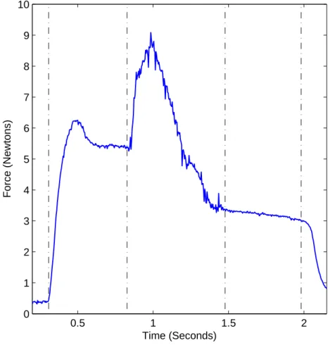
is separated by a vertical line. The first and last sections represent force generation when the muscles are not contracting. The second and fourth sections represent the force generated during an isometric contraction; with the third section denoting the stretch shortening contraction. Note that in the stretch shortening contraction there is an isometric component to force generation, and modeling should estimate both the isometric and stretch shortening components.

We have 86 such force tracings, and investigators wish to model the isometric and stretch shortening force generation. The data are defined as follows: for an individual measurement, 565 evenly spaced functional observations were taken. This measurement was taken two times (pre and post excersize protocol) resulting in 2×565 = 1130 functional measurements per animal. All 43 animals (28 old and 15 young) underwent the same resistive exercise protocol resulting in 48,590 total measurements. Our intent is to investigate possible differences in response, between groups (young/old), as well as differences in response pre- and post-training. We are interested in comparing the individual and group level force tracings for isometric as well as stretch shortening contractions.

(33)

2.1.1 Skeletal Muscle Force

Statistical methods for functional data analysis cannot easily incorporate mecha-nistic information and often produce results that are challenging to interpret. There is a large literature on muscle force output based on differential equations. Such models are easily interpretable and incorporate mechanistic information but are not flexible enough to realistically characterize available data. Motivated by the need to quantify differences in physiological muscle force output as a biomarker of muscle adaptation or pathology (Erdemir et al. 2007), we develop a non-parametric Bayesian modeling approach.

The force generated by muscle activation, illustrated in Figure 2.1, is nonlinear (Maffiuletti 2010; Parsaei and Stashuk 2011) and is associated with complex physiol-ogy, such as motor systems and muscle twitch dynamics. The current lack of accurate statistical models for characterizing force tracings has made effective statistical com-parisons challenging.

Models for isometric force measurements date back to Hill (1938). A popular ap-proach uses first order differential equations relating muscle force output to a series of motor, damper, spring systems (Wexler et al. 1997; Ding et al. 1998; Phillips et al. 2004). Such models may reasonably describe areas of observed data across the force activation curve but do not represent important aspects of the response. Other model-ing approaches (Geronilla et al. 2006) attempt to characterize the response curve usmodel-ing a time-varying combination of basis functions, leading to improvements in prediction but a lack of interpretability and accommodation of prior mechanistic knowledge.

In an effort to develop better training/rehabilitation protocols tailored to individ-ual needs, recent studies have investigated how age affects muscle adaptation and mal-adaptation following specific non-injurious, repetitive, resistance-type loading protocols designed to induce increases in performance and muscle mass. Initial investigations

(34)

(Cutlip et al. 2006; Murlasits et al. 2006) and subsequent validations (Ryan et al. 2008; Baker et al. 2010; Hollander et al. 2010) have supported the use of supramaxi-mal, electrically-evoked stretch-shortening contractions precisely prescribed for induc-ing adaptation (increases in performance and muscle mass) in young animals followinduc-ing repetitive exposures of resistive muscle contractions. We use such data to study the ef-fects of age on resistive muscle training sessions to better understand the benefits/harm of training across age groups.

Complexities arise when modeling the force tracings of a stretch-shortening con-traction. The force output is a product of the isometric force at timet and a function related to joint movement. That is, the total force h(t) measured at time t is thought to be

h(t) =Q(t)F(t), (2.1)

where F : _R+ _→

(35)

2.1.2 Relevant Literature

From a Bayesian perspective there has been some work on estimation of parameters from ODEs. Lunn et al. (2002) develops a framework for parameter estimation in phar-macokinetic/pharmocodynamic models. Putter et al. (2002) developed methods based on partial differential equations to estimate HIV infection, and Huang et al. (2006) de-veloped a hierarchical framework to investigate the antiviral response for HIV infection in a population of individuals. The methods assume that the differential equations are characterized through finitely-many parameters, with posterior computation relying on Metropolis-Hastings steps.

Alternatively, one can rely on a Gaussian process (GP) emulator (Kennedy and O’Hagan 2000; 2001). In the first stage, a solver is used to obtain the differential equa-tion soluequa-tion on a finite grid of points. Then, uncertainty and bias are accommodated in the second stage through centering a GP prior on the differential equation solution. Mechanistic information is not included in the Gaussian process and hence, unless one assumes a very small deviation from the differential equation solution, the resulting trajectories may be quite unrealistic, leading to poor predictive performance. Our goal is to obtain mechanistic hierarchical Gaussian processes, which favor realizations that inherit the behavior of the ODE, while also allowing variability among individual trajectories across subjects.

Recent work (Lawrence et al. 2007; Alvarez et al. 2009; Honkela et al. 2010) devel-ops latent force models, which embed mechanistic information into a GP prior. Here the GP has a mean function and covariance kernel derived from a differential equation similar to that of a simple motor, damper, spring system. This is accomplished by spec-ifying a GP prior with squared exponential covariance function and integrating this GP over the Greens function corresponding to the specified ODE. In our experience, this

(36)

approach cannot be applied directly to our motivating application due to extreme ill-conditioning problems in the covariance matrix. Hence, instead of directly using their methods, we develop an alternative approach that relies on accurately approximating solutions to the differential equations. This method is then extended to a hierarchical Gaussian process (Behseta et al. 2005) allowing for sharing of information among sub-jects in the population. By using the hierarchical Gaussian process we model individual experimental group effects as well as individual subject effects.

2.2 Mechanistic Gaussian Process

Consider modeling an unknown functional responseh:T →_R,withT = [t0, t1]∈R

and data consisting of error-prone measurements (y1, . . . , yn)0ofhat locations (t1, . . . , tn)0.

A common approach lets

y(tl) = h(tl) +l, (2.2)

where h ∼ GP(0, R(·,·)), a zero mean GP with covariance kernel R(·,·), and l iid ∼

N(0, τ−1), with l = 1, . . . , n. The covariance kernel R(·,·) is frequently chosen as squared exponential, exponential, Matern or some default form that leads to flexi-ble realizations. Although prior information about h can potentially be incorporated through the mean of the Gaussian process and choice of the covariance kernel, it can be difficult to choose appropriate values in practice.

We incorporate prior information by defining a covariance kernel favoring shapes consistent with mechanistic information specified by differential equations. We assume the information is expressible in the form of a linear ordinary differential equation

Lh(t) = d

m_h(t)

dtm +am−1(t)

dm−1_h(t)

dtm−1 +. . . a1(t)

dh(t)

(37)

Given {a0(t), . . . , am−1(t)} are non-zero on T, the solution to (2.3) exists and, given

initial values, can be expressed as

h(t) =

Z t

t0

G(t, ξ)r(ξ)dξ. (2.4)

Here G(t, ξ) is Green’s function, and the integral operator R G(t, ξ)dξ, described in shorthand asGbelow, is a linear operator, and is the inverse of the differential operator L in (2.3). As G is linear, ifr(t)∼ GP(0, R(·,·)), then h(t) is also a Gaussian process with a new covariance kernel dependent on G and R(·,·). This defines a GP over h whose covariance kernel favors shapes consistent with (2.3).

Unfortunately, in many cases the resulting covariance matrix is extremely ill condi-tioned resulting in computational instability. We tried a wide variety of existing meth-ods for addressing ill-conditioning problems in GP regression with no success. The induced covariance of h(t) tends to be substantially more subject to ill-conditioning than even the squared exponential covariance. Alternatively, by relying on a Runge-Kutta approximation (Asaithambi 1995), we develop an approach that allows direct modeling of r(t) for an arbitrary covariance kernel R(·,·). In our experience this in-creases the numerical stability of the approximation, while bypassing the cumbersome calculations necessary to compute the covariance kernel.

2.2.1 Approximation of the Process

There is a large literature on approximate solutions to differential equations. Given a set of initial conditions corresponding toh(t0) as well as the firstm−1 derivatives ofh

evaluated at the initial pointt0, Runge-Kutta (RK) methods (see chapter 9 Asaithambi

(1995)) offer efficient algorithms that approximate the solution to an mth _{order ODE.}

When L is linear, RK methods express the numerical solution to the ODE as a linear

(38)

combination of the forcing functionr(t) evaluated at a finite set of points,{tl}nl=1,along

with the initial conditions h∗ = {h∗₁, . . . , h∗_m}. We illustrate the approach using the Euler-Cauchy second order approximation, though other RK approximations proceed in much the same way.

The Euler-Cauchy approximation recursively defines a solution to h(t) at {tl}nl=1,

by approximating the function as a linear combination of r = (r(t1), . . . , r(tn))0 and h∗. As an example, consider a first order differential equation (i.e., m = 1 in (2.3)) where points are equally spaced with ∆ = 2(tj−tl−1).The approximate Euler-Cauchy

solution is formed recursively by:

ˆ

hl =hl−1+ ∆{g(tl−1, hl−1)} (2.5)

hl =hl−1+

∆ 2

n

g(tl−1, hl−1) +g(tl,ˆhl) o

. (2.6)

Hereg(tl−1, hl−1) is a function of the derivative evaluated attl−1 andhl−1 forl >1 (e.g.,

for (2.3) withm= 1 one has g(tl−1, hl−1) = [r(tl−1) +A0(tl−1)hl−1]). As long as g(t, f)

is linear the approximation is a linear function of r(t) and the initial conditions h∗. Consequently the solution can alternatively be expressed as a product of a matrixGand a vector of elements r∗ = (h∗,r0)0. We form the matrix recursively as above, with row l corresponding directly to each function evaluation described above. Continuing with the example, one defines the matrixGas follows: first set the first row toh1 0 · · · 0i, which corresponds to h∗₁. Then for l ≥ 1 the approximation proceeds by specifying a row vector

ˆ

G{l,:} = [1 + ∆A0(tl−1)]G{l−1,:}+ ˆK,

(39)

is the previous row. One then defines rowl of G as

G{l,:} =G{l−1,:} +

∆ 2

h

A0(tl−1)G{l−1,:} +A0(tl−1) ˆG{l,:}

i

+K,

whereKis a row vector of zeros except at entrieslandl+1, which are set to∆₂.Through this alternate expression one arrives at the approximationh(t)≈Gr∗, and h(t) is seen in the context of a linear regression whereh∗ and r are unknown. Though we describe the method using the Euler-Cauchy approximation (a second order method), a similar Gmatrix can be constructed using higher order RK methods. Higher order methods do form better approximations but require more functional evaluations of r(t). This may requirer(t) to be evaluated at points on the index set that have not been observed and may greatly increase the computational complexity when sampling from the posterior. Before implementation this trade off should be evaluated, as in many situations a lower order approximation is adequate. For example numerical experiments produced results that in most cases had a maximum difference of 10−3 _{between the actual and numerical}

solution, indicating higher order solutions were not needed.

2.2.2 Posterior Sampling

For the above approximation, sampling from the mechanistic GP proceeds us-ing a series of conditionally conjugate Gibbs steps. The discussion assumes model (2.2) with Y ∼ N(h, τ) where Y = (y1(t1), . . . , yn(tn)) and h = (h(t1), . . . , h(tn))0,

with τ ∼ Ga(a0, b0). Following the above discussion, the matrix G is formed from A = (A1(t), . . . , An(t))0, which are parameters in (2.3). Further we assume the initial

conditions are specified ash∗ ∼N(A0, B0),which is independent of r(t).

(40)

Sampling algorithm 1

1. Sample r∗ ∼ N(E, W) where W = (τ G0G+ Ω−1₎−1 _and _E ₌_W_{(τ G}0_Y _{+ Ω}−1_ρ).

Here Ω = block-diag(B0,Σ) is an (n+m)×(n+m) matrix, ρ is the the prior

mean ofr∗, and Σ is the n×n covariance matrix, formed from R(·,·). 2. Sample τ fromGa(a0+n/2, b0+ (Y −Gr∗)0(Y −Gr∗)/2).

3. Marginalizing out r∗, i.e., Y ∼N(0, GΩG0+τ−1_{I) where} _I _{is a (n}_×_{n) identity}

matrix, sample the parameters A using a Metropolis-Hastings or griddy Gibbs (Ritter and Tanner 1992) sampling step.

2.3 Adaptation to Muscle Force Application

The mechanistic GP is not directly applicable to the muscle force application, which has the additional complication of decomposing h(t) as

h(t) =

  

 

F(t) t /∈[ta, tb]

F(t)Q(t) t∈[ta, tb]

(2.7)

(41)

2.3.1 Prior Extended to Muscle Force Data

We define an ODE for F(t) and Q(t) using generalizations of models from the muscle force literature. The isometric force function F(t) is historically related to the first order differential equation (Hill 1938)

dF(t)

dt −BF(t) +p(t) = 0. (2.8)

Here B represents the damping constant of the muscle fibers and p(t) corresponds to the joint action of muscle at time t. We assume that the form of the motor activation function is unknown but is linear shortly after activation.

Placing a linearity assumption on p(t) only during the SS contraction, we let

p(t) =

S X

s=0

βsbs(t)

where b0(t) = 1 and bs(t), for s≥1 are defined as piecewise polynomial splines on the

interval Ts = [τs−1, τs+1]. For s 6= s0 we use cubic splines defined to be 0 prior to the

interval and 1 after the interval. Here for all s 6=s0 these intervals are defined outside of the range of the SS contraction. For the interval including the SS contraction we let bs0 be a linear spline on the interval, 0 prior to, and 1 after the SS contraction. In order to model a flexible curve we use a large number of splines in estimating p(t).

When the joint is moved through its range of motion the force on the joint is related to the angle of the joint and other factors. Angular motion is often described using a second order differential equation, and we follow this approach. As the exact form of the differential equation is unknown (i.e., damping constant etc.) we specify this

(42)

function through the fully specified second order differential equation:

d2_Q(t)

dt2 +λ

dQ(t)

dt −AQ(t) +g(t) = 0, (2.9)

where g(t) ∼ GP(0, R(·,·)), A > 0 and the damping constant λ ≤ 0. Note that when g(t) = 0 this defines a periodic function with a period of π√A.

It is further known that the multiplicative effect ofQ(t) should be 1 prior to and after the joint is moved through a stretch shortening contraction. We add the constraint that at the beginningta,and endtb,of the stretch shortening contractionQ(ta) = Q(tb) = 1.

One can easily sample from this using the conditional properties of the multivariate normal distribution.

2.3.2 Posterior Sampling Extensions

The RK approximation is used to sample both F(t) and Q(t). Analogous to h∗

above, we defineF∗ = (F0)0 and Q∗ = (Q0, Q1)0,initial value vectors forF(t) andQ(t)

respectively. Similarly let p = (p(t1), . . . , p(tn))0, and g = (g(t1), . . . , g(tn)),0 which,

as above, are vectors of the latent forcing functions evaluated at a finite set of points for F(t) and Q(t) respectively. Further define p∗ = (F∗0,p0)0 and g∗ = (Q∗0,g0).0 For convenience we refer to G as the Euler-Cauchy approximation to either (2.8) or (2.9). For all references toF(t), G is the solution to (2.8), and for all references toQ(t), Gis the solution to (2.9).

In sampling F(t) we note p = Xβ, where X is the n×(S + 1) matrix of spline basis functions {bs(t)}Ss=0 evaluated at (t1, . . . , tn) and β = (β0, β1, . . . , βS). Letting

(43)

1. Putting the prior F∗ ∼ N(A0, B0) over the initial conditions, define V = GX,

ρ = (A0₀ 0)0, and Ω = block-diag(B0,Σβ). Then sample p∗ ∼ N(E, W), where

W = (τ V0V + Ω−1)−1 and E =W(V0Y + Ω−1ρ).

We modify algorithm 1 to sample g∗ given Q(ta) = Q(tb) = 1. This is done using

the conditional properties of the multivariate normal distribution, i.e., for

   X1 X2  

∼N

      µ1 µ2   ,   

C11 C12

C12 C22      , one has

X1|X2 ∼N µ1−C12C22−1[µ2− X2], C11−C12C22−1C21

(2.10)

In the above approximation Q(ta) = Q0 and Q(tb) = G{n,:}g∗, where G{n,:} is the last

row ofG, we modify step one of sampling algorithm 1 as follows:

1. Calculating g∗ ∼N(E, W) as in algorithm 1, define the following quantities

E∗ =



 

I G{n,:}





E, W

∗ =    I G{n,:}





W

I G{n,:}

.

Then sample g∗|Q(ta)Q(tb) from a normal distribution whose mean and

covari-ance are derived from E∗ and W∗ as in (2.10).

On the interval [ta, tb] sampling Q(t) and F(t) proceeds conditional on knowledge

of the other. To sample F(t) one uses algorithm 2 and multiplies each row of Gby the

(44)

corresponding value of Q(t) (i.e., for row l one multiplies each element in this row by Q(tl)). Similarly we multiply byF(t) when sampling Q(t) and sample from algorithm

3.

2.4 Hierarchical Mechanistic Gaussian Process

We extend the mechanistic GP to hierarchical modeling (Behseta et al. 2005). This allows modeling of individual curves as well as population means. The extension is described in terms of our application but can be readily used in other settings.

Consider a study in which there is a single factor of interest having I levels. For subject j a functional response hijk : T →R is measured K times. In our application

the factor is age,I = 2, K = 2 and represents measurements pre and post exercise rou-tine, andhijk(t) is the time varying force function. Here, for all i, j, k,the n functional

measurements are taken at equally spaced points on the index setT.Data are modeled as:

yijk(tl) = hijk(tl) +ijkl,

whereijkl iid

∼N(0, τ_j−1),and a mechanistic Gaussian process prior is defined overhijk(t)

as in (2.3).

For subjectj, in groupi, the pre and post functional measurements are modeled as

hijk(t) = ˜hij1(t)1(k≥1) + ˜hij2(t)1(k≥2), (2.11)

(45)

0 otherwise. In terms of the mechanistic GP one models the latent forcing function as

rijk(t) = ˜rij1(t)1(k≥1) + ˜rij2(t)1(k ≥2). (2.12)

Here one integrates (2.12) using (2.4) to get (2.11). For interpretability between obser-vations and groups we use the same integral operator Gacross all i, j and k.

Extending (2.12) to account for variability between factors we define

˜

rijk(t)∼ GP(r (1) ik , R

(1) ik (·,·))

r_ik(1) ∼ GP(r_k(2), R(2)_k (·,·)),

with k = 1,2 as in (2.12) and r_k(2) ∼ GP(0, R(3)₍_·_,_·_)). _{Sampling from this hierarchy}

proceeds in much the same way as algorithm 1. Analogous to the case of the single curve we define ˜r∗_ijk, r(1)_ik ∗, and r(2)_ik ∗ as above. Further, we define the individual vector of observations Yijk = (yijk(t1), . . . , yijk(tn))0. Sampling from the posterior is specified

in terms of ˜r∗_ijk, r_ik(1)∗, and r(2)_ik∗, and proceeds as follows: Sampling algorithm 4

1. For each i, j, k sample ˜r∗_ijk conditionally on ˜r∗_ijk0 where k0 = 1 if k = 2 and k0 = 2 otherwise. Here let Y∗ = (Yijk − G˜rijk∗ 0) and sample ˜r∗_ijk ∼ N(E, W) where W = (τ G0G+ Ω−_ijk1)−1_{, E} ₌_W_{(τ G}0_Y∗_{+ Ω}−1

ijkr (1)∗

ik ).Here, as in sampling algorithm

1, Ωijk is subject specific (n+m)×(n+m) covariance matrix.

2. For each i, k pair r(1)_ik ∗ ∼ N(E, W) where in this case W = (P jΩ

−1 ijk+ [Ω

(1) ik ]

−1₎

and

E =WP jΩ˜

−1 ijk˜r

∗

ij + [Ω (1) ik ]

−1_r(2)∗ k

.Here Ω(1)_ik is an (n+m)×(n+m) covariance matrix as specified above, whereR(1)_ik (·,·) is used to compute the finite dimensional covariance for the latent forcing function.

(46)

3. For r(2)_k ∗ sample as in step 2 replacing˜rijk with r (1)∗

ik etc.

4. For each i, j sample τj from Ga(a0+n, b0 + P

k(Yijk−Gr∗ijk)0(Yijk −Gr∗ijk)/2),

wherer∗_ijk=˜r∗_ij₁1(k ≥1) +˜r∗_ij₂1(k ≥2). 5. Sample A similar to algorithm 1.

Note that inference on the group average curvesh(1)_ik (t) and the population average curves h(2)_k (t) proceed using the approximation Gr_ik(1)∗ and Gr(2)_k ∗ respectively, and, as G is the same across all i, j, k, the population averages have the same interpretation as other curves in the hierarchy. Extending the above framework, i.e. adding more hierarchies, is straightforward. Each additional hierarchy is sampled as in step 2 noting that the previous level is used as the input vector.

2.4.1 Extensions to the Hierarchal Mechanistic Process

We extend the hierarchical mechanistic process to our application. Here

hijk(t) =   

 

Fijk(t) t /∈[ta, tb]

Fijk(t)Qijk(t) t∈[ta, tb]

where Fijk(t) and Qijk(t) are defined using (2.8) and (2.9) respectively. For Fijk(t)

and Qijk(t) we define the hierarchy over the latent forcing function, with pijk(t) and

gijk(t) specified as in (2.12). This discussion uses the same notation as above, i.e.,

˜

gijk(t),˜g∗ijk,p˜ijk(t),p∗ijk etc.

For Qijk(t), the forcing functions ˜gijk(t), g (1)

ijk(t), and g (2)

ijk(t), are defined such that

Qijk(ta) = Qijk(tb) = 1 etc, and these constraints are implemented in exactly the same

(47)

Hierarchical extensions in modeling Fijk(t) are direct. Here we place multivariate

normal hierarchies over the spline coefficient vector β vector, i.e:

˜

β_ijk ∼N(β(1)_ik ,Σ(1)_β,ik)

β(1)_ik ∼N(β(2)_k ,Σ(2)_β,k),

which in turn defines ˜pijk(t), p (1)

ik (t), and p (2)

k (t). Sampling each ˜p

∗

ijk,p (1)∗

ik , and p (2)∗

k

proceeds by placing the modifications of sampling algorithm 2 into sampling algorithm 4.

2.5 Simulation

We conduct a simulation experiment based upon the model developed in (2.7). Here curves, similar to those expected in a muscle force application are generated, and the simulated curves are compared against posterior estimated curves. Similar to the muscle force application the hierarchy was generated assumingI = 2, J = 30 and K = 2.The group levels of the hierarchy, i.e.,F_ik(1)(t) andQ(1)_ik (t),were generated to resemble muscle force tracings of isometric and stretch shortening contractions respectively, and were simulated based upon (2.8) and (2.9). The individual level data were generated at 565 equally spaced points, assuming ∆ = ₂₆₀1 . Here the first 80 observations represent the force tracing prior to muscle activation. After activation 120 observations were taken of Fijk(t). The next 201 observations were of Fijk(t)Qijk(t) with the 164 remaining

observations generated from Fijk(t). Similar to the real data, all data was generated

assuming little variability between observations; hereτj = 1000 for all observations.

We chose weakly informative priors for all hyper parameters. We place a GP prior overgijk(t) where the covariance kernel is specified using the squared exponential kernel

K(t, t0) =σ2_exp(₋_`_k_t₋_t0_k2_). _{We set} _σ−2 _∼ _Ga(1,_{1) and let} _`_∼ _Ga(1000,_0.1), _which

(48)

reflects the assumption that gijk(t) is not expected to be very smooth. The same

assumptions are made for all other levels of the hierarchy. For pijk(t) we put normal

priors over the β coefficients, with diffuse priors specified at the topmost level. The precision parameter for all other levels was assigned a Ga(0.1,0.1) prior. Finally the precision parameter τj was specified using a Ga(100,0.1) prior. This is a vague prior

onτj centered approximately at the observed error found in muscle force tracings. For

the parameters in (2.8) and (2.9) we defined discrete uniform priors over a range of plausible values. HereB is defined to be in [4.1,5.2], based upon analyses of isometric data with a parametric parametric model. Further the parameterA, which defines the period ofQijk(t) is put in the range of [−2.3,−0.6].This choice corresponds to a range

representing a half to a full period. Finally the damping constant was expected to be negligible, andλ was given a plausible range of [0.01,1]. Noteλ can not take on values at 0 due to the identifiability constraints on the ODE.

We collected 25,000 MCMC samples disregarding the first 5,000 as a burn-in. Every other observation was then recorded, leaving 10,000 samples for the analysis. Exami-nations of trace plots for the quantities of interest, i.e., the individual curves, as well as curves in the hierarchy, showed excellent mixing. Hyperparameters for the covariance kernel as well as the parameters specified in (2.8) and (2.9), exhibited poor mixing. This however did not affect the convergence for the quantities of interest.

For the quantities of interest (i.e., Fijk(t), Qijk(t), F (1)

ik (t), and Q (1)

ik (t))), which

(49)

where truth is well described by the model.

2.6 Muscle Force Application

With the goal of investigating the effect of non-injurious, repetitive muscle contrac-tions on muscle force generation, we apply our approach to data compiled from Cutlip et al. (2006), Murlasits et al. (2006), and Baker et al. (2010). In these studies, 15 young (3 months), and 28 old (30 months), rats’ dorsiflexor muscles were exposed to a resistive muscle contraction protocol that included thirteen sessions. At the end of each session the dorsiflexor muscle group underwent isometric as well as stretch shortening contraction (as described in Figure 2.1). Individual observations were taken at evenly spaced intervals (∆ = ₂₆₀1 of a second). The entire measurement lasted just over 2 seconds, resulting in 565 total functional observations as in our above simulation study. Our analysis looks at possible differences between muscle force measurements pre (after the first resistive muscle contraction protocol) and post (after the last protocol) study, between young and old animals. Priors for all parameters as well as computational implementation was as specified in the simulation.

Figure 2.3 shows the individual fits of hijk(t) for one animal for their pre and post

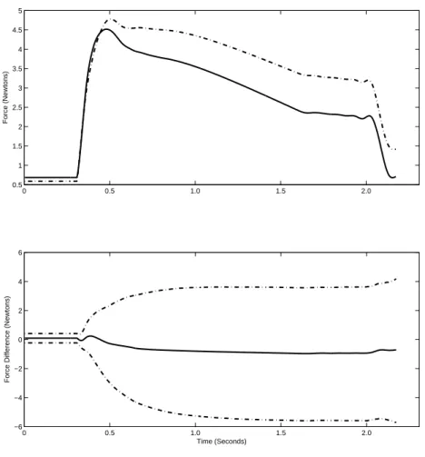
observations. Here the central posterior estimated curve is shown in black, with the observed data shown using gray hash marks. The credible intervals are not shown, as they are too close to the central estimate to be visible in the figure. Figure 2.4 shows the expected mean isometric contraction for the pre (dashed line) and post (solid line) exercise protocol in the old animals (top left) and the young animals (top right). The difference (solid line) between the pre and the post training, as well as the 95% pointwise credible interval (dashed line), is shown in the bottom row for the old (bottom left) and young (bottom right) animals. Here it is seen that the young animals, as a group, displayed increased muscle performance related to stretch

(50)

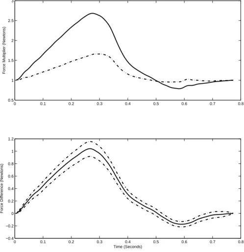
shortening contractions; however, the old animals did not display a difference for much of the curve. When there were differences, they were small and not seen as biologically relevant. Likewise no difference was shown in the group average isometric contraction (i.e.,F_ik(1)(t)). For the group level isometric contractions, figure 2.5 shows the estimated posterior curves (top) and corresponding differences (bottom) for the young animals. Here the pre treatment (dotted line) and post treatment(solid line) estimated isometric contractions are shown in the top row, and, though the central estimates are different, the bottom row shows that there is not enough evidence to suggest differences between the two groups. Similar results (figure not shown) were observed for the older animals. The model also allows one to look at individual estimates between curves. Here though the old animals showed no significant differences at the group level for both iso-metric and stretch shortening contraction force generation, individual differences were seen. Figure 2.6 shows the stretch shortening contraction difference for an individual animal. Here the pre and post treatment estimates are shown in the top graph with the estimated differences being shown in the bottom graph. Here individual differences can be seen, which is significant as it supports the idea that some some older animals vary in their physiology related to dynamic responses.

Note that there is an additional advantage of modeling the latent forcing function as it may be used to generate or support hypotheses. For example, for Fijk(t), the

latent forcing function pijk(t) represents the muscle motor action at time t. These