Sharif University of Technology
Scientia IranicaTransactions D: Computer Science & Engineering and Electrical Engineering www.scientiairanica.com
Spatial diversity gain of MIMO single frequency
network in passive coherent location
M. Radmard
, M. Nazari Majd, M.M. Chitgarha, B.H. Khalaj and M.M. Nayebi
School of Electrical Engineering, Sharif University of Technology, Tehran, Iran.
Received 24 December 2012; received in revised form 23 October 2013; accepted 8 April 2014
KEYWORDS Multi-input multi-output;
Spatial diversity; Single frequency network; Passive coherent location.
Abstract. Recently, it has been shown that applying MIMO technology, i.e. using multiple antennas at the transmit side and multiple antennas at the receive side, improves the performance of object detection and localization. In such scenarios, the spatial diversity specically helps overcome the fading of the cross section of the object, leading to reduced probability of missed detection. Such a phenomenon is, in fact, the dual of probability of bit error reduction in communication systems due to diversity gain. Despite the importance of such performance enhancement, this subject has not been suciently investigated in the PCL (Passive Coherent Location) schemes, where the transmitters (or illuminators of opportunity) used for localization are already present in the environment. Especially, in cases where the transmitters are working in a SFN (Single Frequency Network), such as the DVB-T (Digital Video Broadcasting-Terrestrial) signal, and all are transmitting the same signal, the situation becomes of higher importance. Obviously, the eect of the SFN environment invalidates the assumption of sending orthogonal waveforms traditionally used in localization schemes. In this paper, we design the Neyman-Pearson detector for a PCL scheme and show that we can achieve the desired diversity gain for such a design as well.
c
2014 Sharif University of Technology. All rights reserved.
1. Introduction
1.1. Passive coherent location
PCL has attracted much attention due to its advan-tages over active detection schemes. Low-cost passive localization, which requires no frequency allocation, is a good solution for increased localization at a lower cost [1]. The feasibility of dierent kinds of opportunistic signal used for this application has been investigated earlier, for example, in the case of FM [2], analogue TV [3,4], DTV (Digital TV) [5-7], satellite systems [8], and GSM [9,10]. New digital signals, such
*. Corresponding author. Tel.: +98 21 66163667 E-mail addresses: [email protected] (M. Radmard); [email protected] (M. Nazari Majd);
[email protected] (M.M. Chitgarha); [email protected] (B.H. Khalaj); [email protected] (M.M. Nayebi)
as Digital Audio/Video Broadcast (DAB/DVB), are also excellent candidates [11-13], as they are widely available and can be easily decoded.
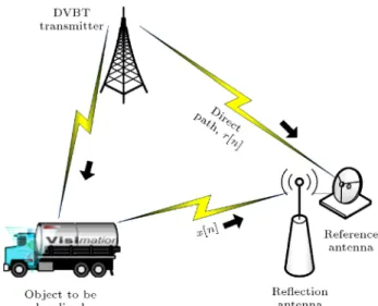
In traditional active systems, the object's range is dened by comparing the time of the transmitted and received pulses. However, such information is not directly available in the case of the PCL. Instead, two antennas are used: one for receiving the signal directly from its main source without reections from objects of interest (reference antenna) and the other for collecting the reections from objects in the environment (reec-tion antenna). Figure 1 depicts the overall structure of the PCL.
Detection is done through computation of CAF (Cross Ambiguity Function) computed according to Eq. (1). It is a criterion of how much correlation exists between the reference and the reection signal. A given CAF's peak in a range-Doppler cell is a representative
Figure 1. Structure of a passive scheme.
of a target in that range and Doppler frequency. j(; )j2= j1
N
N
X
n=1
x(n)r(n )e j2
Nnj2; (1)
where x[n] is the signal at the target channel, r[n] is the reference signal, is the Doppler shift, is the sample shift and N is the number of samples collected. 1.2. Multi-Input Multi-Output (MIMO), an
upcoming technology for localization Recently, use of MIMO techniques for improving the performance of localization schemes has attracted much attention. Generally, such MIMO schemes are divided into two categories: widely separated [14] and colocated antennas [15]. In the former case, multiple transmitters and receivers that are widely separated are used. The main advantage of such conguration is that by obtaining signals from dierent angles, the probabil-ity of missed detection decreases; a concept also known as spatial diversity in MIMO communication. In fact, as shown in [14] the concepts of spatial diversity and multiplexing gain emerge in a manner dual to the ideas in traditional MIMO communication. On the other hand, in the case of colocated antennas, transmitters and receivers are located at nearby positions. Such con-guration is similar to phased array systems, with the dierence that signals emitted by each antenna can be totally uncorrelated with the other antennas. Recent studies have shown that the widely separated antenna conguration leads to enhanced detection performance (Diversity Gain) [16-18], better tracking [19], and higher resolution (spatial multiplexing gain) [20]. On the other hand, improved parameter identiability [21], better target identication and classication [22], di-rect applicability of adaptive arrays for detection and parameter estimation [23,24], and enhanced exibility for transmit beam-pattern design [25,26] are achieved by the colocated antennas conguration.
1.3. MIMO passive coherent location, a new concept
By combining the ideas of passive and MIMO localiza-tion, one can achieve the benets of both schemes by using multiple receivers to detect objects illuminated by multiple noncooperative transmitters. In general, the transmitters may be sending dierent signals (e.g. a broadcasting FM radio with a GSM base station). One case of high interest is the DVB-T SFN (Single Frequency Network), in which all TV transmitters are broadcasting the same data at the same frequency band.
1.4. Diversity gain in MIMO PCL
Multipath fading is one of the most fundamental features of wireless channels. Because multiple received replicas of the transmitted signal sometimes combine destructively, there is a signicant probability of severe fading. Without proper means to mitigate such fading scenarios, ensuring reasonable reliability requires large power margins [27]. One of the most powerful tech-niques to mitigate the eects of fading is to use the di-versity combining of independently fading signal paths. Diversity-combining uses the fact that independent signal paths have a low probability of experiencing deep fades simultaneously. Thus, the idea behind diversity is to send the same data over independent fading paths. These independent paths are combined in such way that the fading eect on the resulting signal is reduced. There are many ways of achieving independent fading paths in a wireless system. One method is to use multiple transmit or receive antennas in an antenna array conguration, where array elements are separated enough in space [28]. Therefore, rather than making the success of a transmission entirely dependent on a single fading realization, the probability of failure is reduced by exploiting multiple such realizations [27], leading to spatial diversity.
Mathematically, in MIMO communication, diver-sity gain is dened at high SNR values as [29]:
lim
SNR!1
log Pe
log SNR = d; (2)
where Peis the error probability and d denotes diversity
gain. It should be noted that in MIMO detection, Pe
is replaced by Pmiss (missed detection probability).
It is well known that if the object to be localized is much greater than the wavelength of a transmitted signal, the received signal will be random and uctu-ating in time. Signal uctuations deteriorate detection performance [30], as the object's cross section parallels the role of the random wireless channel. The reason is that if an object's size is much greater than the wavelength of a transmitting signal, the dierence in distances from scatterers to receiver antennas signif-icantly exceeds the wavelength. Consequently, the
phase of signals arriving from dierent scatterers may uctuate signicantly. Even small random rotations of a real object about its center of mass lead to signicant changes in distance, and hence, sharp phase variations of signals received from dierent scatterers [30]. Cor-respondingly, parallel to MIMO communication, it is possible to obtain diversity by looking at an object from dierent angles.
Obtaining diversity gain in MIMO detection has recently been highly investigated, [17,31,32]. But, such analysis has not yet been performed in the case of applying MIMO to PCL. The main dierence is that here, we use noncooperative transmitters whose transmitted signal is not under control. Especially in a DVB-T network of transmitters, all the transmitters send the same signal in the same frequency.
In previous works on MIMO detection, it is assumed to have active transmit antennas. Mostly, it is assumed that the transmitted waveforms are orthogonal [33-38], so that they can be separated at the receiver side, a property that is not true in the case of MIMO PCL (especially DVB-T, which is almost the focus of PCL because of its unique properties for radar application and also being broadcasted in a network, making it quite suitable for MIMO application). For example, in [31], it is assumed that:
Z 1
1sk(t)s
k0(t)dt
8 < :
1 if k = k0
0 if k 6= k0 (3)
Also, in [32], the authors want to obtain the diversity gain when the waveforms are not orthogonal (but not fully correlated). They use an orthogonal basis to show the non-orthogonal transmitted waveforms, where the dimension of this basis is Mn, which is less or equal
to the number of transmitters (being equal in the case of transmitting orthogonal signals). Finally, they have concluded that:
d = minfNMn; Qg;
where Q is the number of scatterers. However, in our case (MIMO SFN PCL e.g. DVB-T), Mn = 1 (all
of the transmitters are sending the same signal) and, therefore, the diversity gain is not proportional to the number of transmitters, according to the results of the aforementioned paper.
In addition, in [39], the optimal test statistics for a statistical MIMO radar (or equivlently a MIMO radar with widely separated antennas) using non-orthogonal signals are derived. However, the authors in [39] have not considered the fact that dierent paths experience dierent loss paths from the transmitter to the target to the receiver. Indeed, in a MIMO radar with widely separated antennas, the transmitted signals arrive at the receiver with dierent delays and
dierent path losses, which is ignored in the signal model of [39].
In this paper, we want to see if we can obtain the main advantage of the MIMO technique (i.e. diversity gain) in MIMO DVB-T based passive radar (PCL). In Section 2, we will design the detector structure for a MIMO PCL in a single frequency network. Pmiss
will be derived in a closed form, and obtaining a spatial diversity gain proportional to the product of the number of the transmit and receive antennas will be proved. Simulations for dierent environments are included in Section 3. Finally, Section 4 concludes the paper.
2. Detection in the MIMO SFN PCL
Assume that there are M illuminators of opportunity (e.g. broadcasting DVB-T signals in a Single Frequency Network), N receive sensors and an object to be localized. For simplication, we have assumed that the object to be localized has no Doppler, although such an assumption is not critical in our derivations. The reection antenna is assumed to be omnidirec-tional, collecting signals arriving from all directions. An important obstacle in passive coherent location is the Direct Path Interference (DPI), which should be rejected from the reection channel. Dierent schemes to overcome such an eect have been recently presented for PCL systems, where satisfying practical results have been achieved [2,7,40]. Therefore, in this paper, we assume that such schemes have been incorporated and the remaining DPI eect is negligible.
At the receiver side, after DPI cancellation, the signal is passed through a CAF processor to obtain the delays and Doppler frequencies of dierent echoes collected from the object to be localized. The threshold at the output of the CAF processor for declaring that an object is detected is determined by the desired false alarm rate (Pfa). In the case of MIMO PCL, the signal
received at the n'th receive antenna is presented by Eq. (4):
rn(t) =
r Et
L
M
X
i=1
n i
r1ir2is(t i) + n(t); (4)
where s(t) is the transmitted signal (the same for all transmitters), r1i and r2i are the distance from the
transmitter to the target and the distance from the target to the receiver, respectively, M is the number of transmitters, i is the cross-section gain of the object
illuminated by the signal transmitted from the ith transmitter, Etis the energy of the transmitted signal,
L is the channel loss, and i denotes its delay.
We dene the probability of missed detection (Pmiss) as the probability that we miss all echoes of
Pmiss= M
Y
m=1 N
Y
n=1
Pmn
miss; (5)
where Pmn
miss is the probability of missing the object's
echo from the m'th transmitter at the n'th receiver. The reason for considering the case of missing all echoes of the object as missed detection is that we can design the detector such that after detecting one or two echoes, the threshold can be reduced adaptively in order to detect a sucient number of echoes (e.g. in the case of one receiver three echoes). Although, by such an approach Pfa would increase, the data association
algorithm we have developed in [42], used to associate these echoes to objects, will eliminate such false echoes. In fact, the target localization schemes developed for MIMO DVB-T based PCL, such as [42], assume that each object's echo is detected with a given probability of detection. So, even if some (but not all) echoes are missed, it might still be possible to localize the object using the remaining echoes' TDoAs (Time Dierence of Arrival). Such algorithms would denitely fail if no echo from the object is detected at the receiver. However, as the number of detected echoes decreases, the probability of correct localization decreases as well. Another reason is that we can localize the object by other techniques, such as Direction-Of-Arrival (DOA) estimation, after detecting it at an acceptable Pmiss
level. In addition, the reason for multiplying the missed detection probabilities comes from the fact that the antennas are widely separated, resulting in decorrelated echoes [14].
2.1. Problem formulation
Next, we explore the probability of missed detection in the MIMO PCL. The existence of a target in a specic bistatic range cell is a random process with unknown probability. We use a Neyman-Pearson detector because a priori probabilities are unknown. Consequently, we compare the likelihood ratio, L(y), with threshold to derive the false alarm probability. So, at the n'th receiver, for a specic bistatic range cell, we have:
H0: y = n;
H1: y = n + ls; (6)
where y, s and n are discrete samples of signals, rn(t), s(t m) and n(t), with length NT, respectively.
Consequently, y is the received signal vector at the n'th receiver and s is the signal from the m'th transmitter. In general, the signal is complex, i.e. s = s0ej,
where s0 = jsj is real. Multiplying e j by both sides
of Eq. (6), we have:
H0: e jy = y0= e jn = n0;
H1: e jy = y0= e jn + ls0= n0+ ls0; (7)
where n0 denotes complex noise with the same
proper-ties of n. As ls0 is real, only the real part of noise is
important. As a result, the hypothesis test is simplied as below:
H0: y = n; H1: y = n + ls; (8)
where, for simplication, we have denoted Re(y0) by y,
s0 by s, and Re(n0) by n. Therefore, in the rest of the
equations, the signals are real.
It should be noted that the signals presented in other bistatic range cells that make interference in this range cell, are included in n. For example, for the DVB-T signal, which is the case of interest, due to its highly randomized nature, it can be considered as white noise [6,43]. Consequently, the signals of other cells constitute a white noise component for n. Here, we assume the general case of n N (0; R). In subsequent sections, we will consider four dierent cases for R to represent dierent situations of considering noise and clutter.
For H1, where we assume the target is present,
we assume its RCS follows the Swerling I model (also called Rayleigh scatter). If 2 represents RCS, the
distribution function of is: f() = 2
0e
2
220; (9)
where 2
0 is the RCS average value.
In Eq. (8), the coecient l (the gain experienced by the signal from the transmitter to the receiver) is:
l =rv
1ir2i; (10)
where: v =
s
PtGtGrIp2
(4)3LcLr : (11)
In the above equation, Pt is the transmitted power,
Gtand Grare the transmitting and receiving antenna
gains, respectively, Ip is the processing gain at the
receiver, Lcis the scattering loss, and Lris the receiver
loss. Therefore, the distribution function of l is: fL(l) = 2
te
2
22t; (12)
where: 2
t = PtGtGrIp 2 02
(4)3r2
1ir22iLcLr: (13)
fY(yjH0) = fn(y) = 1
(2)NT2 jRj12
e yT R 1y2 ; (14)
fY(yjH1; l) = fn(y ls)
= 1
(2)NT2 jRj12
e (y ls)T R 1(y ls)2 ; (15)
fY(yjH1) =
Z 1
0 fY(yjH1; l)fL(l)dl
= Z 1
0
1 (2)NT2 jRj12
e (y ls)T R 1(y ls)2 l
2 te
l2 22tdl
= e
1 2yTR 1y
(2)NT2 jRj12t2
Z 1
0 e
1
2l2sTR 1s+12l(sTR 1y+yTR 1s) 22l2tldl
= e
1 2yTR 1y
(2)NT2 jRj12t2
Z 1
0 e
1
2l2(sTR 1s+21t)+12l(sTR 1y+yTR 1s)ldl
= e
1 2yTR 1y
(2)NT2 jRj12t2
Z 1
0 e C2
1l2+C2lldl;
(16) where:
C2
1 = 12(sTR 1s +12
t); (17)
C2= 12(sTR 1y + yTR 1s); (18)
so:
fY(yjH1)= e
1 2yTR 1y
(2)NT2 jRj122t
Z 1
0 le
(C1l 2C1C2)2+4C2C22 1dl
= e
1
2yTR 1y+4C2C221
(2)NT2 jRj12t2
Z 1
0 le
(C1l 2C1C2)2dl
= e
1
2yTR 1y+4C2C221
(2)NT2 jRj122tC12
Z 1
C2 2C1
xe x2
dx + Z 1
C2 2C1
C2
2C1e x2
dx !
= e
1
2yTR 1y+ C22 4C21
(2)NT2 jRj122tC12
12e x2
j1
C2 2C1+
p 2C2
2p2C1Q
p 2C2
2C1
!!
; (19) where:
Q(x)= Z 1
x
1 p
2e
u2
2 du; (20)
fY(yjH1) = e
1
2yTR 1y+ C22 4C21
(2)NT2 jRj122tC12
1 2e (
C2 2C1)2+
pC
2
2C1 Q(
C2
p 2C1)
= e
1 2yTR 1y
2(2)NT2 jRj12t2C12
1 +
pC
2
C1 e
C22
4C21Q( pC2
2C1)
! :
(21) The likelihood ratio is dened as below. The detection is done by comparing this ratio with a determined threshold:
L(y) =ffY(yjH1)
Y(yjH0)=
1 22
tC12
1 + p
C2
C1 e
C22
4C21Q( pC2
2C1)
!
: (22)
If L(y) is greater than the threshold, hypothesis H1 is
chosen, otherwise H0:
L(y) ? 1: (23)
Since L(y) is a monotonically increasing function of C2, the previous comparison can be replaced by the
following comparison:
C2? : (24)
Here, we assume R is symmetric (it is a simplication assumption that is consistent with the situations we will consider in the simulations section), i.e.:
RT = R: (25)
Therefore, we have:
C2= sTR 1y ? : (26)
Subsequently, we dene:
v , R 1s: (27)
As a result:
C2= vTy = Ni=1Tviyi? : (28)
lter) matched to v. Now, we can compute Pfa:
T , NT
i=1viyi= vTy: (29)
Under the assumption of H0, T is a linear combination
of NT Gaussian variables. Therefore, it is Gaussian too
and its mean and variance can be obtained as follows: EfT jH0g = EfvTyjH0g = vTEfyjH0g
= Efng = 0; (30)
varfT jH0g = EfT2jH0g = EfvTy yTvjH0g
= vTEfyyTjH
0gv = vTRv
= (R 1s)TR(R 1s) = sTR 1RR 1 s
= sTR 1s: (31)
So under the assumption of the hypothesis H0, T has
the following distribution:
T jH0 N (0; sTR 1s): (32)
The probability of a false alarm can be computed as: Pfa= PrfT > jH0g = Q(p
sTR 1s): (33)
If:
Pfa= ; (34)
then:
=psTR 1sQ 1(); (35)
where is the detector's threshold, which is determined according to the desired Pfa from the above equation.
Now, the probability of detection is computed under the assumption of H1:
T jH1= vTyjH1= vT(n + ls) = vTn + lvTs: (36)
For this n'th receiver, the probability of detecting the signal emitted by the m'th transmitter and then reected by the target can be computed as follows:
Pmn
d = PrfT > jH1g = PrfvTn + lvTs > g
= Z 1
0 Prfv
Tn > vTsxgf
L(x)dx: (37)
From Eq. (27), we have:
PrfvTn > vTsxg = Q(p vTsx
sTR 1s); (38)
vTs = sTR 1s; (39)
PrfvTn > vTsxg = Q( sp TR 1sx
sTR 1s ): (40)
From Eqs. (37) and (39), we can write:
Pmn
d =
Z 1
0 Q
sTR 1sx p
sTR 1s
x
2 te
x2
22tdx: (41)
Substituting the threshold from Eq. (35): Pmn
d =
Z 1
0 Q(Q
1() psTR 1sx) x
2 te
x2 22tdx
= Z 1
0
1 Q(psTR 1sx Q 1()) x
2 te
x2 22tdx
= Z 1
0
x 2 te
x2 22tdx
Z 1
0 Q
p
sTR 1sx Q 1() x
2 te
x2 22tdx
=1 Z 1
0 Q(
p
sTR 1sx Q 1())x
2 te
x2 22tdx;
(42) Pmn
miss=1 Pdmn=
Z 1
0 Q
p
sTR 1sx Q 1()
x
2 te
x2
22tdx; (43)
u , 2x22
t; (44)
Pmn miss=
Z 1
0 Q(
p
sTR 1stp2u Q 1())e udu;
(45) A , t
p
2sTR 1s; (46)
B , Q 1(); (47)
Pmn miss=
Z 1
0 Q(A
p
u B)e udu
= Z 1
0
Z 1
Apu B
1 p
2e
t2 2 dt
e udu; (48)
t > Apu B ) t + BA >pu ) (t + BA )2> u: (49)
displacing the bounds of the two integrals as: Pmn
miss=p12
Z 1
Be
t2 2dt
Z (t+B A )2
0 e
udu
=p1 2
Z 1
Be
t2
2(1 e (t+BA )2)dt
= Q( B) p1
2e B2 A2 Z 1 Be t2(A2+2) 2A2 2tBA2dt
= Q( B) p1
2e
B2
A2+A2(A2+2)2B2
Z 1 Be (t A q A2+2 2 + B
p 2 ApA2+2)
2
dt
= Q( B) p1
2e
B2
A2+A2(A2+2)2B2
r A2
A2+ 2
Z 1
B A
p
A2+2+ 2B ApA2+2
e t022 dt0
= Q( B) r
A2
A2+ 2e
B2 A2+2 Q B A r 4 A2+ 2
p A2+ 2
!! :
(50) Here, we have substituted B and have used the prop-erty of the Q-function:
Q( B) = 1 Q(B) = 1 Q(Q 1()) = 1 ; (51)
Pmn
miss= 1
r k2
k2+ 1e
(Q 1())2 2(k2+1)
Q Qp1() 2k
r 2 k2+ 1
p
2(k2+ 1)
!!
= 1 r
k2
k2+ 1e
(Q 1())2 2(k2+1)
Q
Q 1()
kpk2+ 1(1 (k2+ 1))
= 1 r
k2
k2+ 1e
(Q 1())2 2(k2+1) Q k p
k2+ 1Q 1()
;
(52) where:
k2=A2
2 = t2sTR 1s: (53)
If we dene:
dmn, lim
SNR!1
log Pmn miss
log SNR; (54)
we will deduce (from Eqs. (2) and (5)):
dtotal= Mm=1Nn=1dmn: (55)
Here, by dening the SNR as the ratio of the detector's output in the case of H1to the detector's output in the
case of H0, we have:
SNR = EfTEfT22jy = lsgjy = ng =EfvEf(lvTnnTs)T2vgg
= (vTs)2Efl2g
vTRv =
(sTR 1s)22 t
sTR 1s = 2tsTR 1s;
(56)
k2= SNR; (57)
lim
SNR!1P mn
miss= limk!1Pmissmn = limk!11
r k2
k2+ 1e
(Q 1())2 2(k2+1) Q
k p
k2+ 1Q 1()
; (58) lim k!1 r k2
k2+ 1 = limk!11
1 2k2 + o(
1
k2); (59)
where the denition of o(:) comes from: f(x) = o(g(x)) , lim
x!1
f(x)
g(x) = 0; (60)
lim
k!1e
(Q 1())2 2(k2+1) = lim
k!11
(Q 1())2
2k2 + o(
1 k2):
(61) Using the Taylor series of the Q-function, we have:
Q(x0+ ) = Q(x0) + Q0(x0) + o(); (62)
Q0(x 0) =dxd
Z 1 x 1 p 2e t2 2dtjx=x
0
= p1
2e
x2 2 jx=x
0 =
1 p
2e
x20
2 ; (63)
Q(x0+ ) = Q(x0) p12e
x20
From Eq. (64), we can write: lim
k!1Q
k p
k2+ 1Q 1()
= Q r
k2
k2+ 1Q 1()
!
= Q( Q 1()(1 1
2k2 + o(
1 k2)))
=Q( Q 1()) 1
2k2Q 1()
1 p
2e
(Q 1())2 2
+ o(k12) = 1 2k12Q 1()p1
2e
(Q 1())2 2
+ o(k12): (65)
Using Eqs. (59), (61) and (65), we can write the following for the probability of missed detection:
lim
k!1P mn
miss= 1
1 2k12 + o(k12)
1 (Q 1())2 2k2 + o(
1 k2)
1 1
2k2Q 1()
1 p
2e
(Q 1())2 2 +o(1
k2)
= 1
1 1 + (Q2k21())2
1 1
2k2Q 1()
1 p
2e
(Q 1())2 2 + o( 1
k2)
= (1 )1 + (Q2k21())2 +2k12Q 1()p1
2e
(Q 1())2 2 + o( 1
k2)
= 1
2k2((1 )(1 + (Q 1())2)
+p1
2Q 1()e
(Q 1())2
2 ); (66)
lim
SNR!1log P mn miss= log
1 2
(1 )(1 + (Q 1())2)
+p1
2Q 1()e
(Q 1())2 2
log(SNR); (67)
dmn= lim
SNR!1
log Pmn miss
log SNR = 1: (68)
Therefore:
dtotal= Mm=1Nn=1dmn= MN: (69)
As can be observed, in the MIMO passive coherent location, specically in a single frequency network, the spatial diversity gain is proportional to the product of the number of transmit antennas and the receive antennas.
3. Simulations
In this section, DVB-T stations are used as the non-cooperative illuminators of opportunity, and the DVB-T signal has the same properties as those used in [6]. Also, four dierent cases for the covariance matrix (R) are assumed:
1. White gaussian noise;
2. Colored noise;
3. Clutter;
4. Clutter plus white noise.
In order to verify the results of the previous section, for each case, Pmissvs SNR is depicted for
dif-ferent numbers of antennas at the receive and transmit sides using the Monte-Carlo method.
3.1. White Gaussian noise
When the only interference is white noise, we have: R = 2
nI: (70)
For this case, the detector structure is:
T = sTR 1y ? ; (71)
sTy ? 0= 2
n; (72)
which is the structure of a matched lter: Pfa= Q(p
sTR 1s) = Q(
n
p
sTs); (73)
Pfa= ; (74)
= p
sTs
n Q
1(); (75)
0= n
p
sTsQ 1(); (76)
k2= 2
tsTR 1s = 2 t
2 ns
Ts: (77)
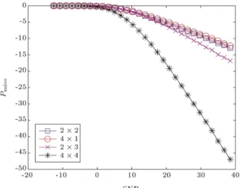
The resulting Pmissis shown in Figure 2. The diversity
Figure 2. Detection performance for the case of white noise.
the MIMO conguration is obvious. Also, as expected from the theoretical results of the previous section, the diversity gain of the two congurations of `two transmitters and two receivers' (2 2) should be equal to the diversity gain of the case of `four transmitters and one receiver' (4 1). This fact is veried in Figure 2, where the slope of the two lines corresponding to the two aforementioned cases are the same at high SNRs.
3.2. Colored noise
In the case of colored noise that we assume here, the noise samples are independent but have dierent energies. So:
R = diag 2
1; 22; : : : ; N2T
; R 1= diag 1
2 1;
1 2
2; : : : ;
1 2 NT
; sTR 1=s1
2 1;
s2
2 2; : : : ;
sNT
2 NT
; (78)
T = NT
i=112
isiyi? ; (79)
which is a lter matched to v =
s1
2 1;
s2
2 2; : : : ;
sNT
2 NT
T : p
sTR 1s =
s NT
i=1s 2 i
2
i; (80)
Pfa = Q(q
NT
i=1s
2 i
2 i
); (81)
Pfa = ; (82)
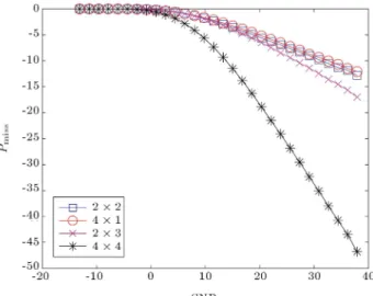
Figure 3. Detection performance for the case of colored noise.
= Q 1()
s NT
i=1s 2 i
2
i; (83)
k2= 2
tsTR 1s = 2tNi=1T s 2 i
2
i: (84)
The results are depicted in Figure 3. As can be easily veried, they are consistent with the expected theoretical results.
3.3. Clutter
In this case, the covariance matrix is as given below:
R = 2 c
2 6 6 6 6 6 6 6 6 6 4
1 : : : NT 1 NT
1 : : : NT 2 NT 1
: : : : : : :
: : : : : : :
NT 1 NT 2 : : : 1
NT NT 1 : : : 1
3 7 7 7 7 7 7 7 7 7 5 ; (85)
where c is the power of the clutter.
The interpretation of the above formula is that the correlation between the samples reduces proportional to (0 < < 1) as their distance increases. As becomes smaller, the signal becomes more stochastic (becomes more similar to white noise, e.g. = 0 corresponds to the white noise case), and, as it grows, the signal becomes more similar to clutter only ( = 1 corresponds to the covariance matrix of the clutter).
Here, the covariance matrix (R) is Toeplitz, which results in:
R 1= 1
2
2 6 6 6 6 6 6 6 6 4
1 0 : : : 0 0
1 + 2 : : : 0 0
0 1 + 2 : : : 0 0
: : : : : : : :
: : : : : : : :
0 0 0 : : : 1 + 2
0 0 0 : : : 1
3 7 7 7 7 7 7 7 7 5 : (86)
After suppressing the energy of clutter using the can-celler at the input of the detector, its power (c) will
be comparable to the noise power. In the simulations, cis chosen 1.5 times the power of noise. Also, we have
chosen = 0:9 for the clutter. v = R 1s =2 1
c(1 2)
2 6 6 6 6 6 6 6 6 4
s1 s2
s1+ (1 + 2)s2 s3
: : :
sNT 2+ (1 + 2)sNT 1 sNT
sNT 1+ sNT
3 7 7 7 7 7 7 7 7 5 : (87)
Therefore, the lter should be matched to the v of Eq. (87):
T =vTy = 1
2
c(1 2)
(s1 s2)y1
+
NXT 2
i=1
si+ (1 + 2)si+1 si+2yi+1
+ ( sNT 1+ sNT) yNT
? : (88)
It can be shown that: T =
NT
X
k=1
bkzk? ; (89)
where: b1= s1
c; bk =
sk sk 1
c
p 1 2;
z1=y1
c; zk =
yk yk 1
c
p
1 2: (90)
In order to compute Pfa, we have:
sTR 1s =XNT k=1
b2 k = (s1
c) 2+XNT
k=2
(sk sk 1)2
2
c(1 2) ; (91)
Pfa= Q(PNT k=1b2k
) ) = Q 1()XNT k=1
b2 k
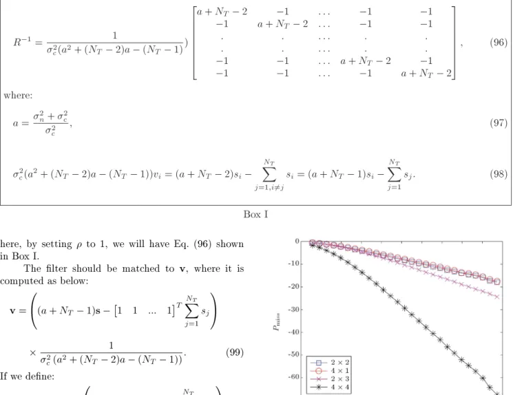
Figure 4. Detection performance for the case of clutter.
= Q 1()
2 4(s1
c) 2+XNT
k=2
sk sk 1
cp1 2
!23
5 ; (92) k2=2
tsTR 1s = 2ti=1NTb2i = 2t
(s1
c) 2
+ NT
i=2(si si 1) 2
2
c(1 2)
: (93)
Figure 4 shows the detector's probability of missed detection for this case. Again, the expected diversity gain is achieved by using multiple antennas in a MIMO conguration.
3.4. Clutter plus white noise In this case:
R = 2 nI + 2c
2 6 6 6 6 6 6 4
1 : : : NT 1 NT
1 : : : NT 2 NT 1
: : : : : : :
: : : : : : :
NT 1 NT 2 : : : 1
NT NT 1 : : : 1
3 7 7 7 7 7 7 5 ; (94) R = 2 6 6 6 6 6 6 4 2
n+ c2 c2 : : : c2NT 1 2cNT
2
c 2n+ c2 : : : 2cNT 2 c2NT 1
: : : : : : :
: : : : : : :
2
cNT 1 c2NT 2 : : : n2+ c2 2c
2
cNT c2NT 1 : : : 2c n2+ c2
3 7 7 7 7 7 7 5 : (95) The earlier assumptions are considered for c, but,
R 1= 1
2
c(a2+ (NT 2)a (NT 1))
2 6 6 6 6 6 6 4
a + NT 2 1 : : : 1 1
1 a + NT 2 : : : 1 1
: : : : : : :
: : : : : : :
1 1 : : : a + NT 2 1
1 1 : : : 1 a + NT 2
3 7 7 7 7 7 7 5
; (96)
where:
a =2n+ 2c
2
c ; (97)
2
c(a2+ (NT 2)a (NT 1))vi= (a + NT 2)si NT X
j=1;i6=j
si= (a + NT 1)si NT X
j=1
sj: (98)
Box I
here, by setting to 1, we will have Eq. (96) shown in Box I.
The lter should be matched to v, where it is computed as below:
v = 0
@(a + NT 1)s 1 1 ::: 1T NT
X
j=1
sj
1 A
1
2
c(a2+ (NT 2)a (NT 1)): (99)
If we dene: G2,sTR 1s =
0
@(a + NT 1)sTs ( NT
X
j=1
sj)2
1 A
1
2
c(a2+ (NT 2)a (NT 1)); (100)
we will have:
Pfa = Q(G) ) = GQ 1()
) = s
(a + NT 1)sTs (PNj=1T sj)2
2
c(a2+ (NT 2)a (NT 1)); (101)
k2= 2
tsTR 1s = 2tG2: (102)
The detector's performance for dierent numbers of antenna at the transmit and receive sides is shown in Figure 5. It veries that using more antennas gives better performance at high SNRs. In addition, in order to verify the theoretical results derived in the previous section, we have compared the Monte-Carlo simulations with the theoretical results of Pmissfor the
case of 2 2 and 4 4 congurations in Figure 6.
Figure 5. Detection performance for the case of clutter plus white noise.
Figure 6. The theoretical results vs the simulation's results.
4. Conclusion
In the Passive Coherent Location (PCL), the objects are detected and localized by the illuminators of op-portunity already present in the environment. The idea of using multiples of these noncooperative transmitters and doing the detection by multiple receive antennas is expected to bring us the advantages of the so-called MIMO systems. An important aspect of such systems is obtaining a spatial diversity gain proportional to the product of the number of transmit and receive antennas. Obtaining this gain was already shown in re-cent research for the case of active transmitters, where the transmit antennas are under control. However, this is not the case when using the illuminators of opportunity of a single frequency network, such as DVB-T. Although such a network is quite interesting for use in a MIMO conguration, transmission of the same signal from all transmitters can degrade the eciency of the MIMO system. The concern arises from recent observations on active transmitters, in which the assumption of sending orthogonal signals, in order to separate them at the receive side, plays a fundamental role in obtaining spatial diversity. In this paper, we show that even in a MIMO PCL working under SFN conditions, the diversity gain of other common MIMO systems can still be obtained.
References
1. Howland, P. \Editorial", Passive Radar Systems, 152(3), pp. 105-106 (2005).
2. Howland, P., Maksimiuk, D. and Reitsma, G. \FM radio based bistatic radar", IEE Proceedings-Radar, Sonar and Navigation, 152(3), pp. 107-115 (2005).
3. Griths, H. and Long, N. \Television-based bistatic radar", IEE Proceedings F- Communications, Radar and Signal Processing, 133(7), pp. 649-657 (2008).
4. Howland, P. \Target tracking using television-based bistatic radar", IEE Proceedings-Radar, Sonar and Navigation, 146(3), pp. 166-174 (2002).
5. Coleman, C., Watson, R., Yardley, H., Coleman, C.J., Watson, R.A. and Yardley, H.A. \Practical bistatic passive radar system for use with DAB and DRM illuminators", In IEEE Radar Conference (2008).
6. Radmard, M., Bastani, M., Behnia, F., Radmard, M., Bastani, M. and Behnia, F. \Cross ambiguity function analysis of the `8k-mode' DVB-T for passive radar application", In IEEE Radar Conference (2010).
7. Saini, R. and Cherniakov, M. \DTV signal ambi-guity function analysis for radar application", IEE Proceedings-Radar, Sonar and Navigation, 152(3), pp. 133-142 (2005).
8. Griths, H., Garnett, A., Baker, C., Keaveney, S., Griths, H.D., Garnett, A.J., Baker, C.J. and
Keaveney, S. \Bistatic radar using satellite-borne il-luminators of opportunity", In International Radar Conference (2002).
9. Tan, D., Sun, H., Lu, Y., Lesturgie, M. and Chan, H. \Passive radar using global system for mobile communication signal: Theory, implementation and measurements", IEE Proceedings - Radar, Sonar and Navigation, 152(3), pp. 116-123 (2005).
10. Sun, H., Tan, D., Lu, Y., Sun, H., Tan, D.K.P. and Lu, Y. \Aircraft target measurements using A GSM-based passive radar", In IEEE Radar Conference (2008).
11. Poullin, D. \Passive detection using digital broad-casters (DAB, DVB) with COFDM modulation", IEE Proceedings - Radar, Sonar and Navigation, 152(3), pp. 143-152 (2005).
12. Daun, M., Koch, W., Daun, M. and Koch, W. \Multi-static target tracking for non-cooperative illuminating by DAB/DVB-T", In OCEANS, 2007-Europe (2007).
13. Daun, M. and Nickel, U. \Tracking in multistatic pas-sive radar systems using DAB/DVB-T illumination", Signal Processing (2011).
14. Haimovich, A., Blum, R. and Cimini, L. \MIMO radar with widely separated antennas", IEEE Signal Processing Magazine, 25(1), pp. 116-129 (2007).
15. Li, J. and Stoica, P. \MIMO radar with colocated antennas", IEEE Signal Processing Magazine, 24(5), pp. 106-114 (2007).
16. Lehmann, N., Fishler, E., Haimovich, A., Blum, R., Chizhik, D., Cimini, L. and Valenzuela, R. \Evaluation of transmit diversity in MIMO-radar direction nd-ing", IEEE Transactions on Signal Processing, 55(5), pp. 2215-2225 (2007).
17. Fishler, E., Haimovich, A., Blum, R., Cimini Jr, L., Chizhik, D. and Valenzuela, R. \Spatial diversity in radars-models and detection performance", IEEE Transactions on Signal Processing, 54(3), pp. 823-838 (2006).
18. De Maio, A. and Lops, M. \Design principles of MIMO radar detectors", IEEE Transactions on Aerospace and Electronic Systems, 43(3), pp. 886-898 (2007).
19. Habtemariam, B., Tharmarasa, R., Kirubarajan, T., Habtemariam, B.K., Tharmarasa, R. and Kirubara-jan, T. \Multitarget track before detect with MIMO radars", In IEEE Aerospace Conference (2010).
20. Fishler, E., Haimovich, A., Blum, R., Chizhik, D., Cimini, L., Valenzuela, R., Fishler, E., Haimovich, A., Blum, R., Chizhik, D., Cimini, L. and Valenzuela, R. \MIMO radar: An idea whose time has come", In IEEE Radar Conference (2004).
21. Li, J., Stoica, P., Xu, L. and Roberts, W. \On pa-rameter identiability of MIMO radar", IEEE Signal Processing Letters, 14(12), pp. 968-971 (2007).
22. Yang, Y. and Blum, R. \MIMO radar waveform design based on mutual information and minimum mean-square error estimation", IEEE Transactions on Aerospace and Electronic Systems, 43(1), pp. 330-343 (2007).
23. Xu, L., Li, J., Stoica, P., Xu, L., Li, J. and Stoica, P. \Radar imaging via adaptive MIMO techniques", In Proc. 14th Eur. Signal Process. Conf. (2006).
24. Wang, H., Liao, G., Liu, H., Li, J. and Lv, H. \Joint optimization of MIMO radar waveform and biased estimator with prior information in the presence of clutter", EURASIP Journal on Advances in Signal Processing, 2011(1), p. 15 (2011).
25. Fuhrmann, D. and San Antonio, G. \Transmit beam-forming for MIMO radar systems using signal cross-correlation", IEEE Transactions on Aerospace and Electronic Systems, 44(1), pp. 171-186 (2008).
26. Stoica, P., Li, J. and Xie, Y. \On probing signal design for MIMO radar", IEEE Transactions on Signal Processing, 55(8), pp. 4151-4161 (2007).
27. Lozano, N. and Jindal, A. \Transmit diversity vs. spatial multiplexing in modern MIMO systems", IEEE Transactions on Wireless Communications, 9, pp. 186-197 (2010).
28. Goldsmith, A., Wireless Communications, Cambridge University Press (2005).
29. Tse, D. and Viswanath, P., Fundamentals of Wireless Communication, Cambridge University Press (2005).
30. Chernyak, V. and Chernyak, V.S. \On the concept of MIMO radar", In IEEE Radar Conference (2010).
31. He, Q., Blum, R. and Haimovich, A. \Noncoher-ent MIMO radar for location and velocity estima-tion: More antennas means betterperformance", IEEE Transactions on Signal Processing, 58(7), pp. 3661-3680 (2010).
32. He, Q. and Blum, R. \Diversity gain for MIMO neyman-pearson signal detection", IEEE Transactions on Signal Processing, 59(3), pp. 869-881 (2011).
33. Badrinath, S., Srinivas, A. and Reddy, V. \Low-complexity design of frequency-hopping codes for MIMO radar for arbitrary Doppler", EURASIP Journal on Advances in Signal Processing (2010). http://asp.eurasipjournals.com/content/2010/1/ 319065
34. Xie, Y., Guo, B., Li, J. and Stoica, P. \Novel multistatic adaptive microwave imaging methods for early breast cancer detection", EURASIP Journal on Applied Signal Processing, 2006(20), pp. 1-13 (2006).
35. Naghibi, T., Namvar, M. and Behnia, F. \Optimal and robust waveform design for MIMO radars in the presence of clutter", Signal Processing, 90(4), pp. 1103-1117 (2010).
36. Feng, D., Li, X., Lv, H., Liu, H. and Bao, Z. \Two-sided minimum-variance distortionless response beam-former for MIMO radar", Signal Processing, 89(3), pp. 328-332 (2009).
37. Chen, J., Gu, H. and Su, W. \A new method for joint DOD and DOA estimation in bistatic MIMO radar", Signal Processing, 90(2), pp. 714-718 (2010).
38. Jin, M., Liao, G. and Li, J. \Joint DOD and DOA es-timation for bistatic MIMO radar", Signal Processing, 89(2), pp. 244-251 (2009).
39. Aittomaki, T. and Koivunen, V. \Performance of MIMO radar with angular diversity under swerling scattering models", IEEE Journal of Selected Topics in Signal Processing, 4(1), pp. 101-114 (2010).
40. Berger, C.R., Demissie, B., Heckenbach, J., Willett, P. and Zhou, S. \Signal processing for passive radar using OFDM waveforms", IEEE Journal of Selected Topics in Signal Processing, 4(1), pp. 226-238 (2010).
41. Radmard, M., Khalaj, B., Chitgarha, M., Nazari Majd, M. and Nayebi, M. \Receivers' position-ing in multiple-input multiple-output digital video broadcast-terrestrial-based passive coherent location", IET Radar, Sonar & Navigation, 6, pp. 603-610 (2012).
42. Radmard, M., Karbasi, S., Khalaj, B. and Nayebi, M. \Data association in multi-input single-output passive coherent location schemes", IET Radar, Sonar & Navigation, 6(3), pp. 149-156 (2012).
43. Raout, J., Santori, A. and Moreau, E. \Passive bistatic noise radar using DVB-T signals", IET Radar, Sonar & Navigation, 4(3), pp. 403-411 (2010).
Biographies
Mojtaba Radmard received BS, MS and PhD de-grees in Electrical Engineering from Sharif University of Technology, Tehran, Iran, where he is currently working as a postdoctoral degree researcher. His research interests include MIMO systems, passive co-herent location, signal processing and speech process-ing.
Mohammad Nazari-Majd received BS and MS de-grees (high honors) in the eld of communications from Sharif University of Technology, Tehran, Iran, where he is currently working towards his PhD degree. His research interests include MIMO radars, noise radars, detection theory and radar signal processing. Mr. Nazari-Majd was also a member of the Iranian Physics' Olympiad team in 2008.
Mohammad Mahdi Chitgarha received BS and MS degrees in the eld of communications from Sharif University of Technology, Tehran, Iran where he is now a PhD degree candidate. He was ranked 1st in both MS and PhD degree national university entrance exams. His research interests include MIMO radars, radar signal processing, detection theory, and speech signal processing.
Babak Hosein Khalaj received his BS degree from Sharif University of Technology, Tehran, Iran, in 1989, and MS and PhD degrees from Stanford University, Stanford, CA, in 1993 and 1996, respectively, all in Electrical Engineering. He joined KLA-Tencor in 1995 as a Senior Algorithm Designer working on advanced processing techniques for signal estimation
and from 1996 to 1999, he was with Advanced Fiber Communications and Ikanos Communications. Since then, he has been a Senior Consultant in the area of Data Communications, and a visiting professor at CEIT, San Sebastian, from 2006 till 2007. Prof. Khalaj has also been senior member of the Ad-vanced Communications Research Institute (ACRI) at Sharif University of Technology, where he has been faculty member since 1999. His main research interests include wireless networking, smart antenna
technologies, sensor networks and digital signal pro-cessing.
Mohammad Mahdi Nayebi received BS and MS degrees from Sharif University of Technology, Tehran, Iran, and PhD degree in Electrical Engineering, from Tarbiat Modarres University, Tehran, Iran.
He joined Sharif University of Technology faculty in 1994. His main research interests are radar signal processing and detection theory.