Sharif University of Technology
Scientia IranicaTransactions B: Mechanical Engineering www.scientiairanica.com
A 3D sliding mode control approach for position based
visual servoing system
M. Parsapour, S. RayatDoost and H.D. Taghirad
Advanced Robotics and Automated Systems (ARAS), Industrial Control Center of Excellence (ICEE), Faculty of Electrical Engineering, K.N. Toosi University of Technology, Tehran, Iran.
Received 5 May 2014; received in revised form 3 September 2014; accepted 20 October 2014
KEYWORDS Nonlinear controller; Position-based visual servoing;
Unscented Kalman lter;
PD-type sliding surface;
Lyapunov theory.
Abstract.The performance of visual servoing systems can be enhanced through nonlinear controllers. In this paper, a sliding mode control is employed for such a purpose. The controller design is based on the outputs of a pose estimator which is implemented on the scheme of the Position-Based Visual Servoing (PBVS) approach. Accordingly, a robust estimator based on unscented Kalman observer cascading with Kalman lter is used to estimate the position, velocity and acceleration of the target. Therefore, a PD-type sliding surface is selected as a suitable manifold. The combination of the estimator and nonlinear controller provides a robust and stable structure in PBVS approach. The stability analysis is veried through Lyapunov theory. The performance of the proposed algorithm is veried experimentally through an industrial visual servoing system.
© 2015 Sharif University of Technology. All rights reserved.
1. Introduction
Visual Servoing (VS) is applied for tracking the move-ment of any specic objects based on a vision input. Dierent research elds, like robotics, image process-ing, and control are applied to achieve VS. It has wide applications in robotics and mechatronic systems like medical robotics, planetary robotics and especially their extensive application in industrial robots [1,2]. The respective control loop in VS has dierent ar-chitectures such as look-and-move structure and per Weiss structure [3]. Look-and-move structure has an internal feedback controller, as being used in many industrial robots. Such setups may accept Cartesian velocity or incremental position commands and permits to simplify the design of control signal [3].
*. Corresponding author. Tel.: +98 21 8846 9084; Fax: +98 21 8846 2066
E-mail addresses: [email protected] (M. Parsapour); [email protected] (S. RayatDoost); [email protected] (H.D. Taghirad)
There are three main approaches in VS [4], Position Based Visual Servoing (PBVS) [5], Image Based Visual Servoing (IBVS) [6], and \2&1/2 D" visual servoing [7], where PVBS is the most frequently used method [5]. In PBVS, the control signal is produced based on the estimation of position and orientation (pose) of the target with respect to the camera. The accuracy of the estimated pose is directly related to the measurement noise and the camera calibration [8]. Extended Kalman Filter (EKF) and Unscented Kalman Filter (UKF) have been developed to deal with the pose estimation in the noisy and uncertain situations. The aforementioned estimators have shown to be quite eective in practice [9-11]. In order to include the velocity and acceleration of the target, the appropriate dynamic model for the relative motion between the camera and the target is necessary. Conventional models are applied based on the constant velocity or the acceleration model which assumes invariable relative velocity or acceleration at each sample time [1].
main goal in VS problem is to enhance the performance of tracking via a controller. Since the system in hand (a robot) has nonlinear dynamics, a nonlinear controller has to be designed for this purpose. For such a design, we use Sliding Mode Control (SMC) in order to achieve the robust performance in the noisy environment as in the industrial environments. Generally, in many forms of VS, the path planning and controlling the end eector of robot are performed separately. By using SMC approach, the aforementioned tasks can be combined together. The combination helps to tune the whole control system together. In SMC, all states of the system are enforced to converge toward a desired sliding surface within a nite time and to stay on this manifold for all further times. In the present paper, we dene a PD-type sliding mode surface to generate a desired path. The novelty of such a selection is the employment of the estimated position, velocity and acceleration of the target for dening the sliding manifold. The estimated values are obtained from a UKF cascade structure which has been recently proposed in [12]. The information of the estimated model and the observation inherits uncertainties which can be directly considered in the proposed controller. The stability of the closed-loop system is proved by Lyapunov theory. As the target object is dynamically changing (in contrast to the pre-planned path), the sliding surface is adapted to the varying positions in the present case.
So far, various types of SMC have been used for VS system in [12-14]. Usually, based on the nonlinear dynamics model of the system, SMC is designed. To the best knowledge of the authors, the stability analysis of the closed-loop system with the combination of the pose estimator in uncertain and noisy situations has not been focused signicantly. SMC for PBVS problem has been introduced theoretically for a 6 DOF robot manipulator in [15]. The desired path is dened in which errors are bounded, and the target visibility is guaranteed. In [16], a sliding surface is designed with the consideration of uncertainties in the nonlinear dynamics of the robot. The proposed algorithm in [17] used dynamics of robot that is too complex to implement on industrial robots. In our case, PD-type sliding surface is developed for a ve degrees of freedom robot manipulator, with PBVS approach. The existence of the internal feedback controller on the industrial robot manipulator makes the controller design simpler, since the robot accepts the position command in the task space. Through the internal loop, a simplied motion kinematics model can be used for the industrial robot, where the controller inputs are the joint velocity signal. To produce the control signal, the information of the pose es-timator is used as the sliding manifold input. Fi-nally, the tracking performance of the adapted control
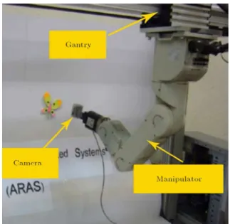
Figure 1. Experimental setup.
scheme on the industrial robot is veried experimen-tally.
2. Theoretical background
In this section, rst the experimental setup, that has been used for VS purpose, is presented. Then, the formulation of UKO+KF pose estimators is reviewed. Furthermore, practical implementation issues of apply-ing control outputs to an industrial manipulator are described.
2.1. Experimental setup
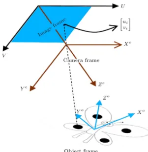
The experimental hardware setup, which is shown in Figure 1, consists of a 5-DOF RV-2AJ robot manipu-lator produced by Mitsubishi Co. augmented with a one degree of freedom linear gantry. This robot has ve degrees of freedom motion, with one degree of redundancy, but the orientation of the wrist about the tool axis is not presented in the structure. Additionally a PC equipped with a Pentium IV (1.84 GHz) processor and a 1 GB of RAM is utilized as the processor. A camera is attached on the end eector of the manipulator, which is a Unibrain Co. product with 30 fs frame rate and a wide lens with 2.1 mm focal length. Since we need a real-time setup, OPENCV Library is used in the Visual Studio environment. 2.2. Feature extraction and pose estimation In the conventional pose estimation, the relative pose of the object with respect to the camera frame in 3D coordinates is calculated. To perform this calculation, some specied points as feature points attached to the target object in 2D coordinates of the image are needed. In Figure 2, the projections of feature points are illustrated in the image frame which is denoted by pim
Figure 2. Camera, object and image frames.
the object frame can be expressed as po
i = (xoi; yoi; zoi);
i = 1; 2; ; n, n 3, and represented in the camera frame by pc
i = (xci; yic; zci). The relationship between pci
and po
i can be dened as the following equation:
pc
i = R(roll, pitch, yaw):poi + T; (1)
in which, roll, pitch and yaw are the orientation Euler angles and the translation are represented by the vector T = [XY Z]T.
Using a pin-hole camera model, the relationship between pim
i and pci can be formulated as follows:
ui
vi
] =h Pfx Pfyi 2 6 4
xc i
zc i
yc i
zc i
3 7
5 ; (2)
where f is the focal length, and Px and Py are
inter-pixel spacing parameters along ui and vi. By folding
the 3n equations (1) into the camera model (2), a set of 2n nonlinear equations is achieved. In order to solve this set of nonlinear equations and achieve a unique solution, at least 3 non-aligned points on the object are required [17]. There are several researches that have applied EKF and UKF for pose estimation [18,19]. Recently, [10] has proposed EKF in addition to KF that guarantees its convergence; however, in [12], it is shown that the performance of this method is directly dependent on the initial condition, and therefore, the employment of UKF instead of EKF leads to a better performance. Due to the promising features of this estimator, this technique has been used as the pose estimator engine in this paper. In this estimator, the nonlinear-uncertain estimation problem is decomposed into a nonlinear-certain observation in addition to a linear-uncertain estimation problem. The rst part is
handled using the Unscented Kalman Observer (UKO) and the second part is accomplished by a Kalman Filter (KF). The pose estimator is fed to a robust and fast modied Principal Component Analysis (PCA) based feature extractor proposed in [12]. This robust method is used in this article to estimate the target pose in an uncertain and noisy environment.
2.3. Singularity avoidance
After estimating the desired dynamic parameter of the target, these parameters have to be converted to the joint space of the robot manipulator. Since there is no prior knowledge on the desired trajectory, and the robot is a ve degrees-of-freedom manipulator, the robot may encounter singular congurations within its prescribed trajectory. To remedy this issue, inverse kinematics of the manipulator is solved in a real-time routine to generate a singular free motion with the consideration of the joint limits for the robot. A practical motion planner, which is proposed by the authors in [20], has been fully elaborated. The applied method shows a well performance when there is no prior information about the via-points and the nal destination of the desired trajectory.
Figure 3 represents the complete loop of the visual servoing system. An image is captured by the camera applied as the input of the \Feature Extractor" block. After estimating the target pose by UKO+KF, the relative pose is commanded to the SMC as a desired position.
3. Design of SMC for PBVS system
The whole process of the VS loop is demonstrated in Figure 4. In the rst step, an image is captured by a camera. Then the desired features are extracted from the mentioned image. After that, the position, velocity and acceleration of the object are estimated by UKO+KF estimator. Error, which is dened as the relative pose, is applied as the input to the sliding surface. Then the control signal (in velocity level) is produced via SMC, which is proportional to each Degree Of Freedom (DOF) of the robot. According to the singularity avoidance, such signals are employed to solve the inverse kinematics problem in order to calculate the angle of each joint. In the nal step, the outcome signal is commanded the internal controller of our industrial robot. Note that, because of the internal
G (X; Y; Z; roll, pitch, yaw) =
ui
vi
; i = 1; 2; ; n; n 3
= 2 6 4
f Px
X+cos(roll)cos(pitch)xo
i+(cos(roll)sin(pitch)sin(yaw) sin(roll)cos(yaw))yoi+(cos(roll)sin(pitch)cos(yaw)+sin(roll)sin(yaw))zoi
Z sin(pitch)xo
i+cos(pitch) sin(yaw)yoi+cos(roll) cos(yaw)zio
f Py
Y+sin(roll) cos(pitch)xo
i+(sin(roll) sin(pitch) sin(yaw)+cos(roll) cos(yaw))yoi(sin(roll) sin(pitch) sin(yaw) cos(roll) sin(yaw))zio
Z sin(pitch)xo
i+cos(pitch) sin(yaw)yoi+cos(roll) cos(yaw)zio
3 7 5 ;
(3) Box I
Figure 4. Block diagram of the overall process.
controller, we can assume the controller as a prefect tracker. The whole process is repeated until the target object is tracked perfectly.
Traditionally, a visual servoing system includes the feature tracking and the feedback controlling as two separate processes. This separation limits tune the whole system performance. In the present paper, we propose to use SMC to perform VS for mentioned tasks. The path planning is accomplished using the sliding mode surface, and the performance is preserved by the sliding mode control output. The stability of the whole control system is proved by Lyapunov theory. Moreover, the robust behavior of SMC against the esti-mation noise provides a suitable tracking performance for the whole visual servoing system.
3.1. Controller design
In this approach, instead of using the dynamics of the system, we have used the estimated values from
UKO+KF and their corresponding desired values to dene the sliding mode surface. The main purpose is tracking a specic object whether the object is moving or not. According to Section 2.1, by substituting Eq. (1) into the pin-hole camera model (Eq. (2)), a set of nonlinear equations is obtained as Eq. (3) and shown in Box I.
These nonlinear equations show the relation be-tween \the relative pose of the target object with respect to the end-eector (camera) frame in the 3D coordinates" and \the feature points attached to the target object in 2D coordinate of the image frame".
By considering a constant velocity model that assumes invariable relative velocity of the target object with respect to the end-eector at each sample time, we may reach the following model for the relative pose of the object with respect to the end-eector:
Wk = AWk 1+ k;
Pk= G(WK) + k; (4)
where:
W=hX; _X; Y; _Y ; Z; _Z; roll; _roll; pitch; _pitch; yaw; _yawiT; and A is a block diagonal matrix with
1 T 0 1
blocks. k and k are the model uncertainty and the
mea-surement noise, respectively, and they are expressed by a zero mean Gaussian noise. Pk is a vector of
the normalized coordinates of the feature points in the image plane.
uiand vi(for at least 3 non-aligned feature points
which are attached to the target object) are calculated by Eq. (2). These points are fed into a UKO to estimate the vector W . The estimation process is explained in [21]. According to the proposed structure in [10,12], the pose vector is estimated by UKO in an iterative loop with the desired stop condition. Here, the estimated velocity is zero, since the same input is used in several epochs. Moreover, utilizing only one set of input data causes an inaccurate estimation. To overcome such a problem, and to estimate the velocity
and acceleration of the object, the UKO output is fed to a linear Kalman lter. Then by changing the output and considering a constant acceleration model that assumes invariable relative acceleration at each sample time, we may reach the following linear model:
Vk = BVk 1+ vk;
Pok = CVk+ k; (5)
where: V =
X; _X; X; Y; _Y ; Y ; Z; _Z; Z; roll; _roll; roll; pitch; _pitch ; pitch; yaw; _yaw; yaw
;
V is the state vector that shows the relative motion parameters between the camera and the target object. B is a block diagonal matrix with
2
41 T 0:5T
2
0 1 T
0 0 1
3 5 blocks. Pok is the pose vector with 6 translational and
rotational elements as X, Y , Z, roll, pitch and yaw. k
and vkare the model uncertainty and the measurement
noise vectors, respectively. vk is related to the static
pose estimator precision. C is a 6 18 matrix with the following format:
cij =
(
1 j = 4i 3
0 otherwise : (6)
Having mentioned the linear model and the desired accuracy of the initial estimation, the KF method is implemented by the recursive formulation to estimate the pose, velocity and acceleration of the target object with respect to the end-eector. After the estimation process, we can dene the desired sliding surface. Let us dene the following PD-type sliding surface:
S =
d dt +
e = _e + e; (7)
in which e is the relative pose of estimated position of the target with respect to the position of the end-eector: and, is the positive constant which species the rate of convergence toward the sliding mode manifold. The sliding surface vector in Eq. (7) is a ve tuple S = sx sy sz sA sBT which
contains the manifold motion variable in x, y and z directions, and orientation about the z and y axis of the robot base coordinate, called in here A, and B orientations, respectively. Based on the relative pose, the state vector is converged toward the sliding surface. Then the state shall smoothly slide on the surface to reach the target state. Because of the movement of
the target, the trajectory path is dynamically changing. Therefore, the position of the current state may diverge from the sliding surface. Hence, the process has to be executed iteratively with a short refreshing period to adapt to the varying positions. There are two approaches to dene the required control signal.
The rst control design is proposed as follows: v1
e e= (t) sgn(S); (8)
in which (t) is a varying time coecient which will be discussed in the next section. sgn(:) denotes the signum function.
The second control signal design is proposed as follows:
v2
e e= 1e + vdes k sgn(S); (9)
in which k is the positive constants; e is the acceleration error between the end-eector and the goal; and, vdes
is the desired velocity of the object.
The rst design consists of only a switching term, while in the second design, a linearizing term is added to the switching term to ensure the sliding condition [22].
3.2. Stability analysis
In the design of the control laws, the sliding condition of the manifold is equal to _e + e = 0 that constrains the motion of the system. Choosing > 0 guarantees that all the states of the system tend to zero as time tends to innity. The rate of the convergence can be controlled by the choice of . The following derivative equation is needed to obtain the control signal:
_S = e+ _e = e+ v1
e e vdes; (10)
where _e represents the dierence between the velocity of the end-eector and the target. Furthermore, ve e
is the end eector velocity, which has been used as the control signal in the practical implementation.
The stability analysis of this algorithm is based on Lyapunov direct method. Consider the following positive denite Lyapunov function candidate V =
1
2STS. To show the stability of this algorithm, the
derivative of the Lyapunov function candidate has to be negative. To provide these circumstances, the control signal has to be limited by a specied function. This function is a subject to the robot velocity constraints and the amplitude of the estimation noise. The following inequality can be specied from Eq. (8). Function '(t) will satisfy the following inequality [23]:
e vdes
1
'(t): (11)
Based on the upper bound of the control signal, the derivative of the Lyapunov function candidate, _S, is
determined by:
_V = S _S = S (e vdes) + Sv1e e; (12)
_V jSj'(t) + Sv1
e e: (13)
By folding the rst control signal Eq. (8) into Eq. (12) the following inequality can be obtained for the derivate of Lyapunov function candidate:
_V jSj'(t) + S( (t) sgn(S)): (14)
With the consideration of (t) '(t) + 0, the
derivative of the Lyapunov function will be semi-negative denite (obviously, _V = 0 when S = 0).
_V 0jSj: (15)
Therefore, the trajectory reaches the manifold S = 0 in the nite time and, once on the manifold, it cannot leave it, as forced by the condition (Eq. (15)).
The same procedure can be done for the second controller design. Combining Eqs. (9) and (12), we have:
_V =S(e vdes)+S 1e+vdes k sgn(S); (16)
_V = kjSj:
In this approach, asymptotic stability is veried by Eq. (16) because the derivate of the Lyapunov function candidate is negative denite.
There are some factors to select one of the con-trollers designs in our practical implementation. The second control design has a linearizing term in contrast to the rst control design. The analysis of the second design can be failed owing to the accuracy estimations in observations, in the presence of uncertainties. On the other hand, the rst design permits to presume un-certainties in more suitable condition for VS problem. In the rst design, (t) is directly determined by the control signal limitations, while in the second design the estimated values from UKO+KF aected such a limitation. Moreover, the command of the robot might be greater than the legal bound of the control signal. Therefore, the rst control design is selected for the practical implementation.
3.3. Modied controller design
SMC has encountered some limitations in practice, especially the chattering [23]. The most conventional modication used to limit the chattering is the bound-ary layer approach [23,24]. To attenuate chattering, the signum function can be replaced by a high-slope saturation function. The control law is altered as:
v1
e e= (t)sat(s="); (17)
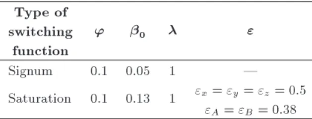
Table 1. The controller parameters. Type of
switching function
' 0 "
Signum 0.1 0.05 1 |
Saturation 0.1 0.13 1 "x= "y= "z = 0:5
"A= "B= 0:38
where sat(:) is the saturation function and " is a positive constant. A suitable approximation requires the use of small ". For the stability analysis, a similar analysis can be performed when jSj ", and the derivatives of the Lyapunov function satises the inequality _V 0jSj. Therefore, whenever jSj ",
jS(t)j will be decreasing, until it reaches the set fjSj "g in a nite time and remains inside thereafter. Inside the boundary layer where jSj ", we cannot have asymptotic stability and only Uniformly Ultimately Bounded (UUB) stability with an ultimate bound can be obtained. The ultimate bound can be reduced by decreasing the depth of the boundary layer [23]. 3.4. Controller parameters selection
According to the constraints of our experimental VS system, the controller parameters are tuned to the selections shown in Table 1. First, based on the tradeo between _e and e from Eq. (7), the rate of convergence () is selected. Then from Eq. (11), with respect to the maximum acceleration of the robot, and the maximum velocity of the goal object, function '(t) is chosen. According to the accuracy of the tracking error, 0 is
selected. The width of the boundary layer (") is tuned in order to reduce the oscillations of the control signal. 4. Experimental results
In this section, the performance of the proposed al-gorithm is veried through a few experiments. In the rst experiment, eciency of visual regulation with two dierent types of switching functions in SMC technique is performed. Second experiment veries the overall performance of the servoing system.
4.1. Experiment I
Visual regulation is performed in this experiment. The pose of the end eector should be regulated accordingly for any arbitrary xed pose of the object. The desired sliding mode manifold is produced based on the error between the estimated pose of the target with respect to the pose of the end eector. The main behavior of the control signal depends on the type of the switching function. Two dierent types of functions, signum and saturation, are employed. To analyze the behavior of these regulations, the initial pose of robot is reset to the same pose for each round of the experiment.
sig-Figure 5. Sliding surface with sign function in (a) X direction, and (b) A orientation.
Figure 6. Control signal with sign function in (a) X direction, and (b) A orientation.
Figure 7. Derivative of Lyapunov function with sign function in (a) X direction, and (b) A orientation.
nal (velocity signal) and the derivative of the Lyapunov function in the X direction and A orientation are shown in Figures 5-7 for signum function, respectively. The X direction and A orientation are selected as the rep-resentatives of translation and orientation respectively, to keep the number of illustrated gures at a managing level. As can be seen in Figure 5(a), the trajectory lies on the sliding surface in the X direction, and converges toward zero (in 0.2 second). The trajectories and the resulting sliding variables reach zero, which indicates that the error of the relative pose tends to zero in 0.8 second and lies on it after the object has been tracked. This issue can be seen in Figure 6, too. The velocity in the X direction is produced as -0.15 cm per second during the rst 0.2 second and after the tracking error tends to zero. The oscillations are due to the chattering; however, the variations remain around zero. This indicates that the controllers have suitably commanded the robot to stay on the sliding surface. As the object has no rotational motion, the control signal and the sliding surface in the A orientation are dithering around zero as shown in Figures 5 and 6(b). Figure 7 shows that the derivative of the Lyapunov
Figure 8. Sliding surface with sat function in (a) X direction, and (b) A orientation.
Figure 9. Control signal with sat function in (a) X direction, and (b) A orientation.
Figure 10. Derivative of Lyapunov function with sat function in (a) X direction, and (b) A orientation.
function is always negative which veries the stability of this algorithm in practice.
In our case, the oscillations cannot signicantly harm the mechanical parts of robot, since they are attenuated through the implemented lters in the inner structure of the robot. In practice, the chattering phenomenon is not desirable. To have a better per-formance in controlling the robot, we have replaced the signum function by the saturation function. The results of this case for the sliding surface, the control signal and the derivative of the Lyapunov function in the X direction and A orientation are shown in Figures 8-10, respectively. The trajectories and the resulting sliding variable reach the desired condition about 0.2 second; however, between 0.2 and 0.5 seconds the tracking errors are not exactly zero, and they are restricted in a bounded region. This is in complete agreement of the stability analysis that guarantees only UUB condition on the tracking errors. In Figure 9, the same behavior can be seen in the control signal, too. The signal is produced in the X direction as 0:22 cm per second and after that, this signal reaches zero in 0.15 second. This signal is not smooth, but the oscillations are signicantly reduced. Since the
Table 2. The obtained relative position from UKO estimator.
Position/ orientation
Initial real value
Initial estimated
value
Final estimated
value
X (cm) 9 9.03 0.25
Y (cm) 6.5 -6.59 -0.24
Z (cm) 28 27.78 18.10
A (deg) -25 -23.91 1.00
B (deg) 0 2.02 0.81
object has no rotational motion, the control signal and the sliding surface are reached zero in 0.15 second. Figure 10 illustrates the derivative of the Lyapunov function which is negative during the end eector movement. This veries the overall stability of this algorithm.
The results of regulating the robot pose from an initial relative pose to the desired position is numerically summarized in Table 2. The estimated values which are shown in Table 2 are from UKO+KF estimator. The \Initial Estimated Value" refers to the relative pose before the end eector movement. The \Final Estimated Value" denotes the relative pose after movement. Before performing Experiment I, the \Initial Real Value" is set manually. By comparing the estimated and the real pose of the target object from this experiment and Experiment II in [12], the nonlinear controller increases the performance of the VS system (i.e. the \Final Estimated Value" for the pose of the object is close to the desired pose). The desired pose dierence between the end eector and the target object is zero in the X, Y directions and A, B orientations, but the distance is 18 cm in the Z
direction (for safety). By assuming stop condition in our algorithm, we prevent the small movement of robot because of the measurement noise around the desired pose. Thus, for the \Final Estimated Value", we will not have exactly zero. The numerical results signify the eectiveness of the suitable applied estimator in the visual regulation methodology.
4.2. Experiment II
The evaluation of the overall performance of the proposed visual servoing technique is the aim of Ex-periment II, which is done through designing a few independent motions of the object. For this purpose, the object is moved in the X, Y , Z, A and B directions. According to the previous experiment, a saturation type SMC with the width of " is considered for Experiment II.
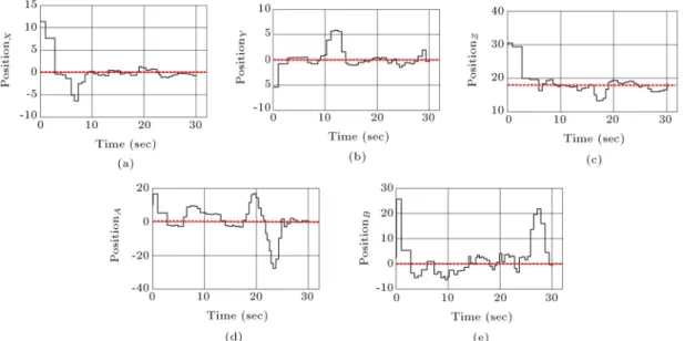
In order to comprehend the experiment better, the estimated relative pose of the target object with respect to the camera frame has been shown in the Fig-ure 11 for all directions, during the object movement. To show the tracking errors performance, Figure 12 depicts the sliding mode surface only in the Y direction and B orientation as samples. Figure 11 shows that when the object moves in any directions, the errors
Figure 12. Sliding surface in (a) Y direction, and (b) B orientation.
Figure 11. UKO+KF estimation of motion in (a) X direction, (b) Y direction, (c) Z direction, (d) A orientation, and (e) B orientation.
with respect to this motion will rapidly grow, and therefore, the corresponding sliding surface will grow. Then, the proposed controller algorithm commands the end eector to move toward the target. For example, focus on Figure 11(a). After 6 seconds, the object is approximately moved -6 cm in the X direction. Proportional to this movement, the sliding surface in the X direction is generated, and the controller compensates these errors. After approximately 4 seconds, the estimated relative pose in the X direction decreases to zero. Similar analysis can be observed for B orientation, as well. Figure 11(e) and 12 show that after 25 seconds, the object starts to rotate around Y axis by about 22 degrees; the estimator detects this rotation. Consequently, the controller rotates the end eector and the errors decrease down to zero. The dash line shows the desired relative pose in each direction, so the robot manipulator is able to keep the desired relative distance. Table 3, shows the performance of the end eector movement, numerically.
To analyze the stability of visual servoing for the moving object, consider Figure 13 that depicts the derivatives of the Lyapunov function which is a suitable measure for the proposed controller strategy. The sliding surfaces in Figure 12 and the derivative of the Lyapunov functions in Figure 13 show non-smooth movement. At the rst glance, the jitters in the plots seem to be non-smooth movement, but if the plot is suitably magnied at the vicinity of jitters, it can be seen that the signal is really smooth. This fact was shown in Experiment I, and the performance is smooth and
Figure 13. Derivative of Lyapunov function in (a) Y direction, and (b) B orientation.
Table 3. Performance of tracking in visual servoing experiment.
Position/ orientation
Initial time of movement
(sec)
Time of tracking (sec)
Compensated relative distance
(cm)
X (cm) 6 10 -6.0
Y (cm) 10 14 +6.0
Z (cm) 16 19 -5.0
A (deg) 19 24 +16.89 & -27.75
B (deg) 25 30 22
proper. Note that, as the target is moved by human, the recorded trajectory includes minute oscillations and vibrations which stems from the human hand motions. For the detail examination of the overall performance of the VS system a video clip is given in: http://saba.kntu.ac.ir/eecd/aras/movies/SMC-Vservo.mpg.
5. Conclusions
In this paper, we present a sliding mode controller in PBVS approach to control and path-plan an industrial robot manipulator. By combining the two mentioned tasks through SMC technique, we can have a unied approach to tune the whole control system in all DOF of robot manipulator. In the proposed approach, the position, velocity and acceleration of the target object are estimated through a robust estimator (UKO+KF). The estimated values are applied to dene a PD-type sliding mode surface. Then a stable and robust SMC is employed to produce a suitable control signal to move the robot toward the desired target. In order to select the controller parameters, we have considered some practical limitations and error bounds, which assume minimization of the relative pose in each DOF of the robot manipulator in hand. In experiments, we have observed that the proposed structure is performing well in noisy backgrounds. It may be concluded, that, this technique can be used for the industrial implementa-tion of a visual servoing system. The idea of using SMC can be extended for IBVS approach. The stability analysis of this algorithm can be investigated under uncertainties, and as a result, controller parameters can be tuned with specic objectives in future work. References
1. Malis, E. and Benhimane, S. \A unied approach to vi-sual tracking and servoing", Robotics and Autonomous Systems, 52(1), pp. 39-52 (2005).
2. Gans, N.R. and Hutchinson, S.A. \Stable visual ser-voing through hybrid switched-system control", IEEE Trans. on Robotics, 23(3), pp. 530-540 (2007).
3. Hutchinson, S., Hager, G.D. and Croke, P.I. \A tuto-rial on visual servo control", IEEE Trans. on Robotics and Automation, 12(5), pp. 651-670 (1996).
4. Chesi, G. and Vicino, A. \Visual servoing for large camera displacements", IEEE Trans. on Robotics, 20(4), pp. 724-735 (2004).
5. Chaumette, F. and Hutchinson, S. \Visual servo con-trol. Part I: Basic approaches", IEEE Robotics and Automation Magazine, 13(4), pp. 82-90 (2006).
6. Malis, E., Mezouar, Y. and Rives, P. \Robustness of image based visual servoing with a calibrated camera in the presence of uncertainties in the three-dimensional structure", IEEE Trans. on Robotics, 26(1), pp. 112-120 (2010).
7. Malis, E., Chaumette, F. and Boudet, S. \2 1/2-D visual servoing", IEEE Trans. Robot. Automat., 15, pp. 238-250 (1999).
8. Wilson, W.J. \Relative end eector control using Cartesian position based visual servoing", IEEE Trans. on Robotics and Automation, 12(5), pp. 684-696 (1996).
9. Taghirad, H.D., Atashzar, S.F. and Shahbazi, M. \A robust solution to three-dimensional pose estima-tion using composite extended Kalman observer and Kalman lter", IET Computer Vision, 6(2), pp. 140-152 (2012).
10. Janabi-Shari, F. and Marey, M. \A Kalman-lter-based method for pose estimation in visual servoing", IEEE Trans. on Robotics, 26(5), pp. 939-947 (2010).
11. Salehian, M., RayatDoost, S. and Taghirad, H.D. \Robust unscented Kalman lter for visual Servoing system", the 2nd International Conference on Control, Instrumentation, and Automation (ICCIA), Shiraz, Iran, pp. 1006-1011 (2011).
12. Stepanenko, Y., Cao, Y. and Su, C.Y. \Variable structure control of robotic manipulator with PID sliding surfaces", International Journal of Robust and Nonlinear Control, 8(1), pp. 79-90 (1998).
13. Zanee, P., Morel, G. and Plestan, F. \Robust vision based 3D trajectory tracking using sliding mode con-trol", Proc. of the IEEE Int. Conf. on Robotics and Automation, 3, pp. 2088-2093 (2000).
14. Kim, J.K., Kim, D.W., Choi, S.J. and Won, S.C. \Image-based visual servoing using sliding mode con-trol", SICE-ICASE International Joint Conference, pp. 4996-5001 (2006).
15. Zanee, P., Morel, G. and Plestan, F. \Robust 3D vision based control and planning", Proc. of the IEEE Int. Conf. on Robotics and Automation, 5, pp. 4423-4428 (2004).
16. Li, F. and Xie, H.L. \Sliding mode variable structure control for visual servoing system", International Jour-nal of Automation and Computing, 7(3), pp. 317-323 (2010).
17. Sim, T.P., Hong, G.S. and Lim, K.B. \Modied smith predictor with DeMenthon-Horaud pose estimation algorithm for 3D dynamic visual servoing", Robotica, 20(6), pp. 615-624 (2002).
18. Yoon, Y. and Kosaka, A. and Kak, A.C. \A new Kalman- lter-based framework for fast and accurate visual tracking of rigid objects", IEEE Trans. on Robotics, 24(5), pp. 1238- 1251 (2008).
19. Wang, J.H. and Chen, J.B. \Adaptive unscented Kalman lter for initial alignment of strapdown iner-tial navigation systems", Proc. of the Ninth Int. Conf. on Machine Learning and Cybernetics, Qingdao, 3, pp. 1384-1389 (2010).
20. Taghirad, H.D., Shahbazi, M., Atashzar, S.F. and RayatDoost, S. \A robust pose-based visual servoing technique for redundant manipulators", accepted for publication in Robotica (May 2015).
21. Wan, E.A. and van der Merwe, R. \The unscented Kalman lter for nonlinear estimation", in Proc. of IEEE Symposium 2000 (AS-SPCC), Lake Louise, Al-berta, Canada, Oct., pp. 153-158 (2000).
22. Slotine, J.E. \Sliding controller design for nonlinear systems", Int. Journal of Control, 40(2), pp. 421-434 (1984).
23. Khalil, H.K., Nonlinear Systems, 3rd Edn., Prentice Hall, Upper Saddle River, New Jersey (2005). Biographies
Mahsa Parsapour received her BSc and MSc degrees in Electrical Engineering from K.N. Toosi University of Technology, Tehran, Iran, in 2011 and 2013, respec-tively. She is currently a researcher at the Advanced Robotics and Automated System (ARAS) group at K.N. Toosi University of Technology, Tehran, Iran. Her research interests are robotics, visual servoing, nonlinear control, and image processing.
Soheil RayatDoost received his BSc degree in Elec-trical Engineering from K.N. Toosi University of Tech-nology, Tehran, Iran, in 2009. After that, he worked as a researcher at the Advanced Robotics and Automated System (ARAS) group at K.N. Toosi University of Technology until 2013. He received his MSc degree from the Department of Electrical and Computer En-gineering, University of Tehran, Iran, in 2014. His current research interests include: pattern recognition, computer vision, aective computing, identication and robotics.
Hamid D. Taghirad received his BSc degree in Mechanical Engineering from Sharif University of Tech-nology, Tehran, Iran, in 1989, his MSc in Mechan-ical Engineering in 1993, and his PhD in ElectrMechan-ical Engineering in 1997, both from McGill University, Montreal, Canada. He is currently a Professor and the dean of the Faculty of Electrical Engineering, and the Director of the Advanced Robotics and Automated System (ARAS) at K.N. Toosi University of Technol-ogy, Tehran, Iran. He is a senior member of IEEE, the chairman of IEEE control system chapter in Iran section member of the board of Industrial Control Center of Excellence (ICCE), at K.N. Toosi University of Technology, editor in chief of Mechatronics Maga-zine, and Editorial board of International Journal of Robotics: Theory and Application, and International Journal of Advanced Robotic Systems. His research interest is robust and nonlinear control applied to robotic systems. His publications include ve books, and more than 190 papers in international Journals and conference proceedings.